Nonlinear Dynamics in Isotropic and Anisotropic Magneto-Optical Traps

Abstract

We briefly review some recent advances in the field of nonlinear dynamics of atomic clouds in magneto-optical traps. A hydrodynamical model in a three-dimensional geometry is applied and analyzed using a variational approach. A Lagrangian density is proposed in the case where thermal and multiple scattering effects are both relevant, where the confinement damping and harmonic potential are both included. For generality, a general polytropic equation of state is assumed. After adopting a Gaussian profile for the fluid density and appropriate spatial dependencies of the scalar potential and potential fluid velocity field, a set of ordinary differential equations is derived. These equations are applied to compare cylindrical and spherical geometry approximations. The results are restricted to potential flows.

1. Introduction

Large samples of alkaline atom clouds can be optically confined by means of magneto-optical traps (MOTs). These traps are composed of a magnetic field gradient (produced by anti-Helmholtz coils) and an intersection of three pairs of orthogonally positioned circularly polarized beams [1,2,3]. The environment that allows the confinement involves the combined effects of magnetic trapping and Doppler cooling mechanisms, which create the potential well and decrease the thermal energy of the samples, respectively. In addition, considering Sisyphus or evaporative cooling techniques also allows sub-Doppler temperatures to be reached. MOTs are important in the task of producing Bose–Einstein condensates [4] and are essential in the realization of optical lattices [5,6] and the observation of collective quantum effects with several self-organized structures [7,8].

When the ratio between the intensities of the incident lasers and their saturation values is sufficiently small, a trapped atomic cloud in an MOT shares similarities with single-component trapped plasmas [9] and astrophysical models for pulsating stars [10]. The fluid modeling of MOTs has been applied [11,12,13,14,15], with hydrodynamic equations subject to harmonic, dissipative and collective forces. The harmonic and dissipative forces originate, respectively, from the Zeeman and Doppler shifts. The collective force is a self-consistent interaction provided by two effects, arising from the imbalance in the absorption of light when the backward and forward laser intensities are locally different and the radiation pressure of scattered photons on nearby atoms [3,16,17,18]. Furthermore, thermal effects are also included.

Attempts to solve the dynamical equations for MOTs rely on linear approximations [11,12,13], specific analytic methods [14,15] and numerical simulations [19,20,21]. Some of these previous results employ radial symmetry assumptions [11,12,13,14]. However, anti-Helmholtz coils create an axially symmetric magnetic field, and this must be reflected in the shape of the atomic cloud [22]. The comparison between axial (anisotropic) and radial (isotropic) symmetry motivates our present analysis of trapped atomic samples.

For this purpose, the minimization of the pertinent action functional is applied, and a Gaussian Ansatz is adopted. This procedure reduces the problem to a set of coupled ordinary differential equations, which can be adapted to axially and radially symmetric MOTs. The analysis of nonlinear systems using variational methods is traditional and simplifies the dynamical equations, as in quantum electron gases [23,24,25] and Bose–Einstein condensates [26,27,28,29,30,31,32]. Due to the Doppler cooling, the lower temperature reached is delimited by the Doppler cooling limit, and the proposed Lagrangian density has a time-dependent exponential factor and is linearly dependent on the velocity potential. The present review is mainly based on [11,12,13,14,15]. The present numerical simulations have slightly different numerical parameters in comparison to [14,15], but they are still compatible with present-day experiments [33,34,35].

It is of much interest to compare the results from hydrodynamic and kinetic approaches. From the very beginning, the kinetic modeling requires a more detailed knowledge of the microscopic state of the atoms, including the distribution of velocities, as well as the macroscopic averages of number density and velocity in a given spatial position, among other moments, as in fluid theory. In this respect, the kinetic approach for MOTs as proposed in [36] is certainly more complete. At the same time, the fluid approach is less demanding from the computational, analytical and experimental points of view. The importance of anisotropic configurations should be noted from the kinetic modeling of [36], in agreement with the fluid modeling. It should be also remarked that the Lagrangian approach in the next section requires the potential flow (see before Equation (5)). Therefore, vorticity is precluded, with implications for the development of possible turbulent or unstable states (see also [37,38]).

This paper is organized as follows. Section 2 contains the starting fluid model and proposes an adequate Lagrangian formalism for the model. Setting reasonable variational functions within the Lagrangian density, a set of ordinary differential equations is derived, describing the damped Kohn oscillations of the center of mass of the atomic cloud, together with the nonlinear oscillations of the width parameters of the atomic cloud. Section 3 discusses the axial and spherical symmetry approximations in terms of the nonlinear dynamical system obtained from the variational method. Section 4 is the concluding section.

2. Model and Time-Dependent Variational Method

The hydrodynamic equations for cold trapped atoms in an MOT are

$$\frac{\partial n}{\partial t}+\nabla ·\left(n\mathbf{v}\right)=0,$$

(1)

$$\frac{\partial \mathbf{v}}{\partial t}+(\mathbf{v}·\nabla )\mathbf{v}=-\nu \mathbf{v}-\frac{1}{mn}\nabla p-\frac{1}{m}\nabla V_h+\frac{1}{m}\nabla V_c,$$

(2)

$${\nabla }^2{V}_c=Qn.$$

(3)

Equations (1)–(3) are, respectively, the continuity, momentum and Poisson equations. These equations describe cold atoms (atomic mass m), with a number density $n=n(\mathbf{r},t)$ and a fluid velocity field $\mathbf{v}=\mathbf{v}(\mathbf{r},t)$, where $V_h=m({\omega }_x^2{x}^2+{\omega }_y^2{y}^2+{\omega }_z^2{z}^2)/2$ is a confining potential provided by the Zeeman shift. The self-consistent scalar potential $V_c$ is the contribution of two independent effects that tend to expand and compress the atomic cloud. The compression arises from the imbalance of the absorption of light, since the backward and forward laser intensities are locally different. The expansion arises from the repulsive interactions of the rescattering photons of neighboring atoms [2,33]. These contributions can be formally expressed as the Poisson equation with the effective charge of the atoms given by $Q=\sqrt{ϵ}=\sqrt{{ϵ}_0({\sigma }_R-{\sigma }_L){\sigma }_L{I}_0/c}$, where ${ϵ}_0$ is the vacuum permittivity, c is the speed of light and $I_0$ is the total intensity of the six laser beams, while ${\sigma }_L$ and ${\sigma }_R$ represent the absorption and reabsorption cross sections, respectively [17]. In typical experiments [33,34,35], the repulsion dominates over the attractive force, so that $Q>0$. For the sake of generality, a polytropic equation of state $p=n_0{k}_{B}T{(n/n_0)}^{\gamma }$ is assumed, where $\gamma$ is a generic polytropic index, $n_0$ is a reference number density and $k_{B}T$ is a reference thermal energy, with $k_B$ denoting the Boltzmann constant. For definiteness, the results are restricted to $\gamma \ge 1$.

In the low-saturation regime, the angular frequency and the damping coefficient can be written in terms of the atomic transitions and confinement parameters,

$${\omega }_z=\sqrt{2}{\omega }_{\perp }={(2\nu \mu /k_L)}^{\frac{1}{2}},\nu =-\frac{8\hslash k_L^2{s}_{\mathrm{inc}}\Delta }{m\mathrm{\Gamma }{(1+4{\Delta }^2/{\mathrm{\Gamma }}^2)}^2},$$

(4)

where $k_L$ is the amplitude of the laser wave vector, ℏ is the reduced Planck constant, $\Delta$ is the detuning frequency between the laser frequency and the atomic transition frequency and $\mathrm{\Gamma }$ is the natural line width of the transition used in the cooling process. In addition, $\mu ={\mu }_B{B}_0/\hslash$, where ${\mu }_B$ is the Bohr magneton and $B_0$ is the intensity of the gradient field. The numerical factor $\sqrt{2}$ in the axial frequency comes from the configuration of the magnetic field created by a pair of anti-Helmholtz coils, namely $\mathbf{B}=B_0(x{\widehat{e}}_x+y{\widehat{e}}_y-2z{\widehat{e}}_z)$[39], so that ${\omega }_x={\omega }_y={\omega }_{\perp }$. For the other forms of magnetic traps, it is necessary to derive appropriate expressions of the confinement force. In MOTs, the red detuning ($\Delta <0$) provides $\nu >0$.

The set of equations given as Equations (1)–(3) for potential flows ($\mathbf{v}=\nabla \theta$), where $\theta =\theta (\mathbf{r},t)$ is the velocity potential, can be obtained by the minimization of the action functional $S=\int dt{d}^{3}r\mathcal{L}$ specified by the Lagrangian density

$$\mathcal{L}=e^{\nu t}\left\{mn\left[\frac{1}{2}{|\nabla \theta |}^2+\frac{\partial \theta }{\partial t}+\nu \theta \right]+n(V_h-V_c)-\frac{{(\nabla V_c)}^2}{2Q}+\gamma k_{B}T\int dn\int \frac{n^{\gamma -2}}{n_0^{\gamma -1}}dn\right\},$$

(5)

where the independent fields are $\theta (\mathbf{r},t)$, $n(\mathbf{r},t)$ and $V_c(\mathbf{r},t)$. Indeed, the use of the Euler–Lagrange equations with respect to the fields $\theta$, n and $V_c$, respectively, yields the continuity, momentum and Poisson equations.

A normalized Gaussian Ansatz is adopted,

$$\begin{array}{c}\hfill n(\mathbf{r},t)=\frac{A}{{\alpha }_x{\alpha }_y{\alpha }_z}{e}^{-\frac{{\rho }^2}{2}},\end{array}$$

(6)

where $A=N/{\left(2\pi \right)}^{\frac{3}{2}}$, N is the number of confined atoms and

$$\rho (\mathbf{r},t)=\sqrt{\frac{{(x-d_x\left(t\right))}^2}{{\alpha }_x^2\left(t\right)}+\frac{{(y-d_y\left(t\right))}^2}{{\alpha }_y^2\left(t\right)}+\frac{{(z-d_z\left(t\right))}^2}{{\alpha }_z^2\left(t\right)}}.$$

(7)

The Gaussian Ansatz reflects the localized atomic cloud and is more amenable to an analytic treatment [23,24]. The time-dependent coordinates $d_i\left(t\right)$ and ${\alpha }_i\left(t\right)$, with $i=x,y,z$, respectively, give the position of the center of mass and the width of the atomic cloud in the different directions. Moreover, the number density is defined as $n_0=N/\left({\alpha }_{x0}{\alpha }_{y0}{\alpha }_{z0}\right)$, where ${\alpha }_{i0}={\alpha }_i\left(0\right)$. At equilibrium, an MOT with a large number of atoms $N>{10}^8$ is expected to have a uniform rather than a Gaussian density [1]. However, the Gaussian Ansatz is much more amenable to analytical calculations, especially in anisotropic cases. For similar simplicity reasons, flat-top uniform densities in MOTs have been fitted by Gaussians [37].

From the continuity equation, the velocity field is given by

$$v_i=\frac{{\dot{\alpha }}_i}{{\alpha }_i}(r_i-d_i)+{\dot{d}}_i$$

(8)

where $v_i$ is the i-component of the fluid velocity field. Hence the velocity potential in the Lagrangian density can be written as

$$\theta =\sum _i\left(\frac{{\dot{\alpha }}_i}{2{\alpha }_i}{(r_i-d_i)}^2+{\dot{d}}_i(r_i-d_i)\right),$$

(9)

where an extra, purely time-dependent additive contribution was ignored since it does not contribute anything.

In addition, the Poisson equation admits an approximate solution given by

$$V_c=-\sqrt{\frac{\pi }{2}}\frac{QA}{{\left({\prod }_j{\alpha }_j\right)}^{\frac{1}{3}}}\frac{\mathrm{Erf}\left(\frac{\rho }{\sqrt{2}}\right)}{\rho },$$

(10)

where $\mathrm{Erf}\left(s\right)=(2/\sqrt{\pi }){\int }_0^s{e}^{-s^{\prime 2}}d{s}^{\prime }$ denotes the error function of a generic argument s. This approximation is more accurate in the case where ${\alpha }_x\simeq {\alpha }_y\simeq {\alpha }_z$, i.e., in the spherical approximation. This condition was discussed in [15].

In order to obtain the equation of motion of the new coordinates, the Lagrangian is obtained after substitution of Equations (6), (9) and (10) into Equation (5), yielding

$$\begin{array}{c}\hfill L[d_i,\dot{d_i},{\alpha }_i,\dot{{\alpha }_i}]\equiv -\frac{1}{mN}\int \mathcal{L}{d}^{3}r=e^{\nu t}\left[\sum _i\frac{1}{2}\left(({\dot{d_i}}^2+{\dot{{\alpha }_i}}^2)-\nu {\alpha }_i\dot{{\alpha }_i}\right)-U_d-U_{\alpha }\right],\end{array}$$

(11)

where

$$U_d=\sum _i\frac{{\omega }_i^2}{2}{d}_i^2$$

(12)

$$U_{\alpha }=\sum _i\left(\frac{{\omega }_i^2}{2}{\alpha }_i^2+b\frac{{\left({\prod }_j{\alpha }_j\right)}^{\frac{1}{3}}}{{\alpha }_i^2}\right)+\frac{a_{\gamma }}{{\left({\prod }_j{\alpha }_j\right)}^{\gamma -1}}.$$

(13)

with

$$b=\frac{NQ}{8{\pi }^{\frac{3}{2}}m},a_{\gamma }=\frac{k_{B}T{\alpha }_0^{3(\gamma -1)}}{{\left(2\pi \right)}^{\frac{3}{2}(\gamma -1)}{\gamma }^{\frac{3}{2}}(\gamma -1)m}.$$

(14)

where $U_d$ and $U_{\alpha }$ are the pseudopotentials corresponding to the dipole and oscillating width modes. Notice that the isothermal case ($\gamma =1$) deserves a separate treatment. The introduced constants b and $a_{\gamma }$ are related, respectively, to the self-consistent interaction and the thermal effects. The value of $a_{\gamma }$ depends on the polytropic index. These equations are valid for $\gamma >1$.

Given the Lagrangian, the equations of motion can be derived by means of the Euler–Lagrange equations. The dynamics of the center of mass is given by

$${\ddot{d}}_i+\nu {\dot{d}}_i+{\omega }_i^2{d}_i=0,$$

(15)

which, as can directly be seen, is decoupled from the width equations showing damped oscillations around the origin (damped Kohn oscillations). Furthermore, this motion is linear and independent of the number of atoms.

The equations of motion for the oscillating widths are

$${\ddot{\alpha }}_x+\nu {\dot{\alpha }}_x+\left({\omega }_x^2-\frac{{\nu }^2}{2}\right){\alpha }_x=\frac{(\gamma -1)a_{\gamma }}{{\alpha }_x^{\gamma }{\left({\alpha }_y{\alpha }_z\right)}^{\gamma -1}}+\frac{b}{3}\left(\frac{5{\alpha }_y^{1/3}{\alpha }_z^{1/3}}{{\alpha }_x^{8/3}}-\frac{{\alpha }_y^{1/3}}{{\alpha }_x^{2/3}{\alpha }_z^{5/3}}-\frac{{\alpha }_z^{1/3}}{{\alpha }_x^{2/3}{\alpha }_y^{5/3}}\right),$$

(16)

$${\ddot{\alpha }}_y+\nu {\dot{\alpha }}_y+\left({\omega }_y^2-\frac{{\nu }^2}{2}\right){\alpha }_y=\frac{(\gamma -1)a_{\gamma }}{{\alpha }_y^{\gamma }{\left({\alpha }_x{\alpha }_z\right)}^{\gamma -1}}+\frac{b}{3}\left(\frac{5{\alpha }_x^{1/3}{\alpha }_z^{1/3}}{{\alpha }_y^{8/3}}-\frac{{\alpha }_x^{1/3}}{{\alpha }_y^{2/3}{\alpha }_z^{5/3}}-\frac{{\alpha }_z^{1/3}}{{\alpha }_x^{5/3}{\alpha }_y^{2/3}}\right),$$

(17)

and

$${\ddot{\alpha }}_z+\nu {\dot{\alpha }}_z+\left({\omega }_z^2-\frac{{\nu }^2}{2}\right){\alpha }_z=\frac{(\gamma -1)a_{\gamma }}{{\alpha }_z^{\gamma }{\left({\alpha }_x{\alpha }_y\right)}^{\gamma -1}}+\frac{b}{3}\left(\frac{5{\alpha }_x^{1/3}{\alpha }_y^{1/3}}{{\alpha }_z^{8/3}}-\frac{{\alpha }_x^{1/3}}{{\alpha }_y^{5/3}{\alpha }_z^{2/3}}-\frac{{\alpha }_y^{1/3}}{{\alpha }_x^{5/3}{\alpha }_z^{2/3}}\right).$$

(18)

As can be seen from Equations (16)–(18), the oscillating widths are described by coupled nonlinear damped oscillator equations. The nonlinearity, which appears on the right-hand side of the equations, arises from the repulsive interaction terms due to the polytropic pressure $(\sim$$a_{\gamma })$ and the collective force described by the self-consistent interaction $(\sim$b). These repulsive effects are counterbalanced by the effective harmonic force ∼$({\omega }_i^2-{\nu }^2/2)$. The system (16)–(18) generalizes the results obtained previously in [15]. In the following, we restrict ourselves to ${\omega }_i>\nu /\sqrt{2}$ (periodic oscillations), which can be satisfied by standard MOT parameters, and we also take $\gamma =5/3$ for the sake of illustration, which corresponds to the usual tridimensional adiabatic coefficient.

3. Results

3.1. Anisotropic MOT

In the anisotropic case with cylindrical symmetry provided by the shape of the magnetic field created by a pair of anti-Helmholtz coils, it is valid to take ${\omega }_x={\omega }_y={\omega }_{\perp }$ and ${\alpha }_x={\alpha }_y={\alpha }_{\perp }$. Consequently, with $a_{5/3}=9\sqrt{3}{k}_{B}T{\alpha }_0^2/\left(20\sqrt{5}\pi m\right)$, the equations of motion become

$${\ddot{\alpha }}_{\perp }+\nu {\dot{\alpha }}_{\perp }+\left({\omega }_{\perp }^2-\frac{{\nu }^2}{2}\right){\alpha }_{\perp }=\frac{2a_{5/3}}{3{\alpha }_{\perp }^{7/3}{\alpha }_z^{2/3}}+\frac{b}{3}\left(\frac{4{\alpha }_z^{1/3}}{{\alpha }_{\perp }^{7/3}}-\frac{1}{{\alpha }_{\perp }^{1/3}{\alpha }_z^{5/3}}\right)$$

(19)

and

$${\ddot{\alpha }}_z+\nu {\dot{\alpha }}_z+\left({\omega }_z^2-\frac{{\nu }^2}{2}\right){\alpha }_z=\frac{2a_{5/3}}{3{\alpha }_{\perp }^{4/3}{\alpha }_z^{5/3}}+\frac{b}{3}\left(\frac{5{\alpha }_{\perp }^{2/3}}{{\alpha }_z^{8/3}}-\frac{2}{{\alpha }_{\perp }^{4/3}{\alpha }_z^{2/3}}\right),$$

(20)

or

$${\ddot{\alpha }}_{\perp }+\nu {\dot{\alpha }}_{\perp }=-\frac{1}{2}\frac{\partial U}{\partial {\alpha }_{\perp }},{\ddot{\alpha }}_z+\nu {\dot{\alpha }}_z=-\frac{\partial U}{\partial {\alpha }_z},$$

(21)

where $U=U({\alpha }_{\perp },{\alpha }_z)$ is the pseudopotential defined by

$$\begin{array}{c}\hfill U({\alpha }_{\perp },{\alpha }_z)=({\omega }_{\perp }^2-{\nu }^2/2){\alpha }_{\perp }^2+\frac{({\omega }_z^2-{\nu }^2/2){\alpha }_z^2}{2}+\frac{a_{5/3}}{{\alpha }_{\perp }^{4/3}{\alpha }_z^{2/3}}+b\left(\frac{2{\alpha }_z^{1/3}}{{\alpha }_{\perp }^{4/3}}+\frac{{\alpha }_{\perp }^{2/3}}{{\alpha }_z^{5/3}}\right),\end{array}$$

(22)

present in the associated Lagrangian function $L=exp\left(\nu t\right)[(1/2)(2{\dot{\alpha }}_{\perp }^2+{\dot{\alpha }}_z^2)-U]$.

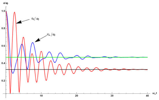
Taking typical MOT parameters [1,3,21,33,34,35,40], Equations (19) and (20) can be numerically solved. These parameters are: $n_0={10}^{15}{\mathrm{m}}^{-3}$, $m=1.41\times {10}^{-25}\mathrm{kg}$ (rubidium), $Q\sim {10}^{-37}{\mathrm{Nm}}^2$, ${\omega }_{\perp }=240\mathrm{rad}/\mathrm{s}$ and $\nu =65{\mathrm{s}}^{-1}$, for $|\Delta |=3.0\mathrm{\Gamma }$, where $\mathrm{\Gamma }=2\pi \times 4\mathrm{MHz}$, $k_L\sim {10}^7{\mathrm{m}}^{-1}$, $s_{inc}=0.05$, $|\nabla B|=10\mathrm{G}/\mathrm{cm}$, $k_B{T}_{lim}=\hslash \mathrm{\Gamma }({\Delta }^2+{\mathrm{\Gamma }}^2/4)/\left(2\right|\Delta \left|\mathrm{\Gamma }\right)=4.07\times {10}^{-27}\mathrm{J}$ and ${\alpha }_0=1.0\mathrm{mm}$. The resulting damped nonlinear oscillations are shown in Figure 1. The equilibrium values are found from the conditions

$$\frac{\partial U}{\partial {\alpha }_{\perp }}=\frac{\partial U}{\partial {\alpha }_z}=0,$$

(23)

or

$$\left({\omega }_{\perp }^2-\frac{{\nu }^2}{2}\right){\alpha }_{\perp \mathrm{eq}}-\frac{2a_{5/3}}{3{\alpha }_{\perp \mathrm{eq}}^{7/3}{\alpha }_{z\mathrm{eq}}^{2/3}}-\frac{b}{3}\left(\frac{4{\alpha }_{z\mathrm{eq}}^{1/3}}{{\alpha }_{\perp \mathrm{eq}}^{7/3}}-\frac{1}{{\alpha }_{\perp \mathrm{eq}}^{1/3}{\alpha }_{z\mathrm{eq}}^{5/3}}\right)=0$$

(24)

and

$$\left({\omega }_z^2-\frac{{\nu }^2}{2}\right){\alpha }_{z\mathrm{eq}}-\frac{2a_{5/3}}{3{\alpha }_{\perp \mathrm{eq}}^{4/3}{\alpha }_{z\mathrm{eq}}^{5/3}}-\frac{b}{3}\left(\frac{5{\alpha }_{\perp \mathrm{eq}}^{2/3}}{{\alpha }_{z\mathrm{eq}}^{8/3}}-\frac{2}{{\alpha }_{\perp \mathrm{eq}}^{4/3}{\alpha }_{z\mathrm{eq}}^{2/3}}\right)=0,$$

(25)

which can be numerically solved. For the present parameters, $a_{5/3}=3.20\times {10}^{-9}{\mathrm{m}}^4/{\mathrm{s}}^2$ and $b=1.59\times {10}^{-8}{\mathrm{m}}^3/{\mathrm{s}}^2$, and the equilibrium values reached due to attenuation are ${\alpha }_{\perp \mathrm{eq}}=0.47\mathrm{mm}$ and ${\alpha }_{\perp \mathrm{eq}}=0.33\mathrm{mm}$, as shown in Figure 1.

3.2. Isotropic MOT

For the radial symmetry approximation, one has ${\omega }_{\perp }={\omega }_z={\omega }_r$. Then, it is possible to assume ${\alpha }_{\perp }={\alpha }_z={\alpha }_r$. This approximation leads to the following equation of motion:

$$\ddot{{\alpha }_r}+\nu \dot{{\alpha }_r}+\left({\omega }_r^2-\frac{{\nu }^2}{2}\right){\alpha }_r=\frac{2a_{5/3}}{3{\alpha }_r^3}+\frac{b}{{\alpha }_r^2}$$

(26)

or

$$\ddot{{\alpha }_r}+\nu \dot{{\alpha }_r}=-\frac{1}{3}\frac{\partial U}{\partial {\alpha }_r},$$

(27)

where $U=U\left({\alpha }_r\right)$ is the pseudopotential defined by

$$\begin{array}{c}\hfill U\left({\alpha }_r\right)=\frac{3({\omega }_r^2-{\nu }^2/2){\alpha }_r^2}{2}+\frac{a_{5/3}}{{\alpha }_r^2}+\frac{3b}{{\alpha }_r},\end{array}$$

(28)

present in the associated Lagrangian function $L=exp\left(\nu t\right)[3{\dot{\alpha }}_r^2/2-U]$.

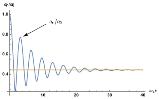
Figure 2 shows the simulation results for Equation (26) for the same parameters as in the previous section. Solving

$$\frac{\partial U}{\partial {\alpha }_r}=0$$

(29)

or

$$\left({\omega }_r^2-\frac{{\nu }^2}{2}\right){\alpha }_{r\mathrm{eq}}-\frac{2a_{5/3}}{3{\alpha }_{r\mathrm{eq}}^3}-\frac{b}{{\alpha }_{r\mathrm{eq}}^2}=0$$

(30)

for the given parameters yields the equilibrium at ${\alpha }_{r\mathrm{eq}}=0.44\mathrm{mm}$, as shown in Figure 2.

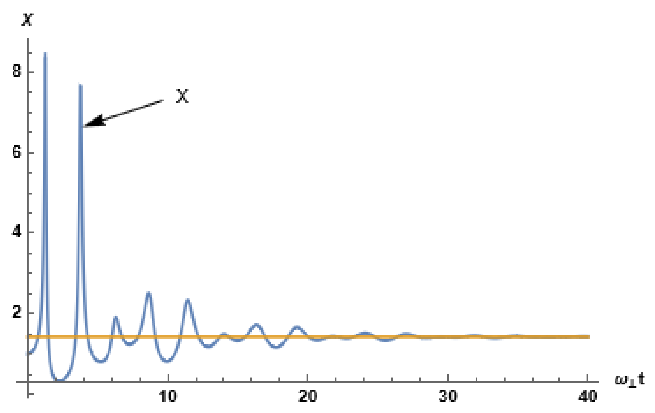
For a better comparison between the anisotropic and isotropic MOTs, it is useful to consider a dimensionless function measuring the anisotropy,

$$\chi =\frac{{\alpha }_{\perp }}{{\alpha }_z},$$

(31)

where $\chi =1$ for the spherical approximation. This is shown in Figure 3, using the same parameters as in Figure 1. It can be seen that the anisotropy can be quite strong from the beginning of the oscillations, reaching an equilibrium value $\chi =1.42$ far from isotropy, contrary to the spherical symmetry assumption. This value is consistent with ${\alpha }_{\perp \mathrm{eq}}=0.47\mathrm{mm}$ and ${\alpha }_{z\mathrm{eq}}=0.33\mathrm{mm}$, as previously found from the stationary states. Furthermore, the use of this approximation forces the magnitude of the magnetic field to be equal in all directions, which contradicts Gauss’s law for magnetism.

4. Conclusions

In this work, the nonlinear dynamics of trapped atomic clouds in anisotropic and spherical MOTs was briefly reviewed. Our treatment was restricted to quadrupole fields created by a pair of anti-Helmholtz coils, producing an azimuthal symmetric confinement harmonic force. The set of partial differential equations for the fluid modeling of the system was converted into a set of Newtonian-like ordinary differential equations for the atomic cloud, using a variational method. The basic equations for the axially and spherically symmetric three-dimensional variational descriptions were derived, when thermal and multiple scattering effects were both relevant. For this purpose, the starting point was a set of hydrodynamic equations with a polytropic equation reinterpreted in terms of the minimization of an action functional, adopting a Gaussian Ansatz. The results were applied to typical experiments, and damped coupled nonlinear oscillations were observed for the model with axial symmetry. For typical experimental conditions using a pair of anti-Helmholtz coils, one can obtain very anisotropic atomic clouds. In the present work, the scattering force was assumed to be always stronger than the shadow force, implying a repulsive collective force. Future studies considering the opposite case are desirable, since instabilities in a (balanced) MOT have their mechanism enhanced for a larger shadow force in comparison with the rescattering [36]. Further possibilities involve the determination of the normal modes and instabilities of dynamical systems such as Equations (19) and (20). In the case of very weak attenuation, another avenue could be the search for additional constants of motion besides the Hamiltonian in these conservative systems.

References

- Labeyrie, G.; Michaud, F.; Kaiser, R. Self-Sustained Oscillations in a Large Magneto-Optical Trap. Phys. Rev. Lett. 2006, 96, 023003. [Google Scholar] [CrossRef] [PubMed]
- Di Stefano, A.; Fauquembergue, M.; Verkerk, P.; Hennequin, D. Giant Oscillations in a Magneto-Optical Trap. Phys. Rev. A 2003, 67, 033404. [Google Scholar] [CrossRef]
- Townsend, C.G.; Edwards, N.H.; Cooper, C.J.; Zetie, K.P.; Foot, C.J.; Steane, A.M.; Szriftgiser, P.; Perrin, H.; Dalibard, J. Phase-Space Density in the Magneto-Optical Trap. Phys. Rev. A 1995, 52, 1423. [Google Scholar] [CrossRef] [PubMed]
- Anderson, M.H.; Ensher, J.R.; Matthews, M.R.; Wieman, C.E.; Cornell, E.A. Observation of Bose-Einstein Condensation in a Dilute Atomic Vapor. Science 1995, 269, 198. [Google Scholar] [CrossRef] [PubMed]
- Guidoni, L.; Verkerk, P. Optical Lattices: Cold Atoms Ordered by Light. J. Opt. B Quantum Semiclass. Opt. 1999, 1, R23. [Google Scholar] [CrossRef]
- Bloch, I. Ultracold Quantum Gases in Optical Lattices. Nat. Phys. 2005, 1, 23. [Google Scholar] [CrossRef]
- Stellmer, S.; Pasquiou, B.; Grimm, R.; Schreck, F. Laser Cooling to Quantum Degeneracy. Phys. Rev. Lett. 2013, 110, 263003. [Google Scholar] [CrossRef] [PubMed]
- Labeyrie, G.; Tesio, E.; Gomes, P.M.; Oppo, G.L.; Firth, W.J.; Robb, G.R.M.; Arnold, A.S.; Kaiser, R.; Ackemann, T. Optomechanical Self-Structuring in a Cold Atomic Gas. Nat. Photonics 2014, 8, 321. [Google Scholar] [CrossRef]
- Manfredi, G.; Hervieux, P.-A. Adiabatic Cooling of Trapped Non-Neutral Plasmas. Phys. Rev. Lett. 2012, 109, 255005. [Google Scholar] [CrossRef] [PubMed]
- Cox, J.P. Theory of Stellar Pulsation; Princeton University Press: Princeton, NJ, USA, 1980. [Google Scholar]
- Terças, H.; Mendonça, J.T.; Kaiser, R. Driven Collective Instabilities in Magneto-Optical Traps: A Fluid-Dynamical Approach. Europhys. Lett. 2010, 89, 53001. [Google Scholar] [CrossRef]
- Terças, H.; Kaiser, R.; Mendonça, J.T.; Loureiro, J. Collective Oscillations in Ultracold Atomic Gas. Phys. Rev. A 2008, 78, 013408. [Google Scholar]
- Terças, H.; Mendonça, J.T. Polytropic Equilibrium and Normal Modes in Cold Atomic Traps. Phys. Rev. A 2013, 88, 023412. [Google Scholar] [CrossRef]
- Soares, L.G.F.; Haas, F. Nonlinear Oscillations of Ultra-Cold Atomic Clouds in a Magneto-Optical Trap. Phys. Scr. 2019, 94, 125214. [Google Scholar] [CrossRef]
- Soares, L.G.F.; Haas, F. Dynamics and Stability of Axially Symmetric Atomic Clouds in Magneto-Optical Trap. Acta Phys. Pol. A 2021, 139, 6. [Google Scholar] [CrossRef]
- Sesko, D.W.; Walker, T.G.; Wieman, C.E. Behavior of Neutral Atoms in a Spontaneous Force Trap. J. Opt. Soc. Am. B 1991, 8, 946. [Google Scholar] [CrossRef]
- Walker, T.; Sesko, D.; Wieman, C. Collective Behavior of Optically Trapped Neutral Atoms. Phys. Rev. Lett. 1990, 64, 408. [Google Scholar] [CrossRef]
- Steane, A.M.; Chowdhury, M.; Foot, C.J. Radiation force in the magneto-optical trap. J. Opt. Soc. Am. B 1992, 9, 2142. [Google Scholar] [CrossRef]
- De Oliveira, R.S.; Raposo, E.P.; Vianna, S.S. Numerical Study of Magneto-Optical Traps through a Hierarchical Tree Method. Phys. Rev. A 2004, 70, 023402. [Google Scholar] [CrossRef]
- Fioretti, A.; Molisch, A.F.; Müller, J.H.; Verkerk, P.; Allegrini, M. Observation of Radiation Trapping in a Dense Cs Magneto-Optical Trap. Opt. Commun. 1998, 149, 415. [Google Scholar] [CrossRef]
- Arnold, A.S.; Manson, P.J. Atomic Density and Temperature Distributions in Magneto-Optical Traps. J. Opt. Soc. Am. B 2000, 17, 497. [Google Scholar] [CrossRef]
- Gajda, M.; Mostowski, J. Three-Dimensional Theory of the Magneto-Optical Trap: Doppler Cooling in the Low-Intensity Limit. Phys. Rev. A 1994, 49, 4864. [Google Scholar] [CrossRef] [PubMed]
- Haas, F. Variational Method for the Three-Dimensional Many-Electron Dynamics of Semiconductor Quantum Wells. AIP Conf. Proc. 2012, 1421, 100. [Google Scholar]
- Hurst, J.; Lévêque-Simon, K.; Hervieux, P.A.; Manfredi, G.; Haas, F. High-Harmonic Generation in a Quantum Electron Gas Trapped in a Nonparabolic and Anisotropic Well. Phys. Rev. A 2016, 93, 205402. [Google Scholar] [CrossRef]
- Manfredi, G.; Hervieux, P.A.; Haas, F. Nonlinear Dynamics of Electron–Positron Clusters. New J. Phys. 2012, 14, 075012. [Google Scholar] [CrossRef]
- Haas, F.; Eliasson, B. Time-Dependent Variational Approach for Bose–Einstein Condensates with Nonlocal Interaction. J. Phys. B 2018, 51, 175302. [Google Scholar] [CrossRef]
- Adhikari, S.K. Finite-Well Potential in the 3D Nonlinear Schrödinger Equation: Application to Bose-Einstein Condensation. Eur. Phys. J. D 2007, 42, 279. [Google Scholar] [CrossRef]
- Ghosh, T.K. Vortex Formation in a Slowly Rotating Bose-Einstein Condensate Confined in a Harmonic-plus-Gaussian Laser Trap. Eur. Phys. J. D 2004, 31, 101. [Google Scholar] [CrossRef]
- Salasnich, L. Time-Dependent Variational Approach to Bose–Einstein Condensation. Int. J. Mod. Phys. B 2000, 14, 1. [Google Scholar] [CrossRef]
- Salasnich, L. Generalized Nonpolynomial Schrödinger Equations for Matter Waves under Anisotropic Transverse Confinement. J. Phys. A 2009, 42, 335205. [Google Scholar] [CrossRef]
- Perez-Garcia, V.M.; Michinel, H.; Cirac, J.I.; Lewenstein, M.; Zoller, P. Dynamics of Bose-Einstein Condensates: Variational Solutions of the Gross-Pitaevskii Equations. Phys. Rev. A 1997, 56, 1424. [Google Scholar] [CrossRef]
- Perez-Garcia, V.M.; Michinel, H.; Cirac, J.I.; Lewenstein, M.; Zoller, P. Low Energy Excitations of a Bose-Einstein Condensate: A Time-Dependent Variational Analysis. Phys. Rev. Lett. 1996, 77, 5320. [Google Scholar] [CrossRef] [PubMed]
- Anwara, M.; Faisal, M.; Ahmed, M. An Experimental Investigation of the Trap-Dynamics of a Cesium Magneto-Optical Trap at High Laser Intensities. Eur. Phys. J. D 2013, 67, 270. [Google Scholar] [CrossRef]
- Gattobigio, G.L.; Michaud, F.; Labeyrie, G.; Pohl, T.; Kaiser, R. Long Range Interactions between Neutral Atoms. AIP Conf. Proc. 2006, 862, 211. [Google Scholar]
- Chanelière, T.; He, L.; Kaiser, R.; Wilkowski, D. Three Dimensional Cooling and Trapping with a Narrow Line. Eur. Phys. J. D 2006, 46, 507. [Google Scholar] [CrossRef]
- Gaudesius, M.; Zhang, Y.-C.; Pohl, T.; Kaiser, R.; Labeyrie, G. Three-Dimensional Simulations of Spatiotemporal Instabilities in a Magneto-Optical Trap. Phys. Rev. A 2022, 105, 013112. [Google Scholar] [CrossRef]
- Gaudesius, M.; Kaiser, R.; Labeyrie, G.; Zhang, Y.-C.; Pohl, T. Instability Threshold in a Large Balanced Magneto-Optical Trap. Phys. Rev. A 2020, 101, 053626. [Google Scholar] [CrossRef]
- Boudot, R.; McGilligan, J.P.; Moore, K.R.; Maurice, V.; Martinez, G.D.; Hansen, A.; de Clercq, E.; Kitching, J. Enhanced Observation Time of Magneto-Optical Traps using Micro-Machined Non-Evaporable Getter Pumps. Sci. Rep. 2020, 10, 16590. [Google Scholar] [CrossRef]
- Pérez-Ríos, J.; Sanz, A.S. How does a Magnetic Trap Work? Am. J. Phys. 2013, 81, 836. [Google Scholar] [CrossRef]
- Devlin, J.A.; Tarbutt, M.R. Laser Cooling and Magneto-Optical Trapping of Molecules Analyzed using Optical Bloch Equations and the Fokker-Planck-Kramers Equation. Phys. Rev. A 2018, 98, 063415. [Google Scholar] [CrossRef]
Publisher’s Note: MDPI stays neutral with regard to jurisdictional claims in published maps and institutional affiliations. |
© 2022 by the authors. Licensee MDPI, Basel, Switzerland. This article is an open access article distributed under the terms and conditions of the Creative Commons Attribution (CC BY) license (https://creativecommons.org/licenses/by/4.0/).