Article

An Investigation of the Resonant and Non-Resonant Angular Time Delay of e-C60 Elastic Scattering

Department of Physics, Indian Institute of Technology Patna, Bihta 801103, India
*
Author to whom correspondence should be addressed.
Atoms 2022, 10(3), 77; https://doi.org/10.3390/atoms10030077
Submission received: 27 June 2022 / Revised: 19 July 2022 / Accepted: 21 July 2022 / Published: 25 July 2022
(This article belongs to the Special Issue Electron Scattering from Atoms, Ions and Molecules)

Abstract

:
Time delay in electron scattering depends on both the scattering angle θ and scattered electron energy E. A study on the angular time delay of e-C60 elastic scattering was carried out in the present work. We employed the annular square well (ASW) potential to simulate the C60 environment. The contribution from different partial waves to the total angular time delay profile was examined in detail. The investigation was performed for both resonant and non-resonant energies, and salient characteristics in the time delay profile for each case were studied.

1. Introduction

Understanding the structure of atoms and molecules received a new insight after the first Coulomb scattering experiment of α particles from gold atoms [1]. Successively, many scattering experiments were conducted, which paved the way for the formulation of Bohr’s atomic model and, consequently, for modern quantum mechanics [2]. For example, experiments by Frank and Hertz provided validation of the discrete nature of atomic energy levels as proposed in Bohr’s theory [3]. Furthermore, the wavelength of electrons was measured for the first time in 1927 by C. J. Davisson and L. H. Germer through a diffraction experiment, confirming the wave nature of matter/particles [4]. Developments in the formulation of the scattering theory of projectiles by atomic/molecular targets go back to the 1930s [5,6]. Since then, scattering studies have undergone rapid development, and scattering now has become a subject of active research. In short, scattering studies, both from experimental and theoretical perspectives, played a dominant role in the development of science in exploring the micro/nano-world, as well as the whole universe [7].
One of the vital attributes of the collision process is the scattering resonance. The physical interaction of the projectile–target coupling can be analysed using quantum scattering resonances. Shape resonance in scattering cross-section indicates that the projectile-target complex is forming a quasi-bound state, resulting in a temporal delay [8]. Studies involving shape resonance have gained massive acceptance due to their wide range of applicability in several fields of physics, such as condensed matter physics [9], biological science [10,11], quantum transportation phenomena at nanoscale structure [12], and cold atom physics [13] etc. Needless to say, the quantum scattering resonance plays an important role in the analysis of target-projectile interaction.
Among the many targets studied through scattering, allotropes of carbon have secured an important position due to their demand for characterisation in a wide variety of research fields. Fullerene-C60, a highly stable molecule with 12 pentagonal and 20 hexagonal carbon rings, attracted the scientific community’s attention. The C60 molecule was reported for the first time in 1985 by Kroto et al. [14]. The possibility of the encapsulation of atoms or small molecules within the C60 molecule enhanced the importance of the molecule; soon after the discovery of the C60 molecule, the endohedral fullerenes were also reported [15]. Endohedral fullerenes are C60 molecules with atoms/ions/molecules trapped inside them and are represented by A@C60, where A denotes the encaged species. The dynamics of fullerenes and their endohedral compounds are explored using collision studies both in theory and experiment [16,17,18,19]. Apart from their fundamental application, fullerenes and their endohedrals have been proposed to be useful in trending technologies. For instance, endohedral fullerenes and nanoparticle lattices have both been recognised as promising key components in future electronic, magnetic, and optical devices [20]. Furthermore, these compounds find applications in medical imaging [21], cancer therapy [22], quantum computing [23], nanoscience [24], materials science [25], etc. They are used in organic photovoltaic devices to enhance their efficiency [26], as well as in electric vehicles as a hydrogen storage material [27]. Jahn-Teller metals, which are rubidium atoms encaged in C60, were reported to exhibit superconductivity at high temperatures [28]. Traces of C60 and its ionic derivatives were also found in interstellar environments [29,30,31,32]. With regards to these stupendous applications, experimental and theoretical studies on fullerenes and their derivatives were carried out on large scales. Some of the notable experimental works on scattering studies from C60 include low-energy elastic e-C60 scattering performed by Tanaka et al. [17], intermediate-energy elastic scattering performed by Hargreaves et al. [33], and high-energy collision studies on fullerene performed by Caldwell et al. [34].
Among the many attributes of scattering, such as total cross-section (TCS), differential cross-section (DCS), partial cross-section (PCS), etc., the scattering time delay has garnered recent attention because it allows characterisation of the projectile–target interaction in the temporal domain. It is assumed that scattering interaction is instantaneous in response to the incident projectile. However, in reality, attoseconds (as) of delay in the time scale are needed for the specific interaction. This means that compared to the projectile that does not feel the scattering centre, the scattered particles experience a time lag or time advancement. The idea of time delay was introduced a few decades back by Eisenbud (1948) [35], Wigner (1955) [36], and Smith (1960) [37]; the parameter is known as Eisenbud–Wigner–Smith (EWS) time delay. Developments made in laser technology have even enabled exploring the dynamics of atoms and molecules in their natural time scale [38,39]. Recently, with the advent of more sophisticated experimental setups, the attosecond time delay was reported in photoionisation from Ar [40,41,42]. Along with experiments, theoretical investigations on time delay are also aplenty [43,44]. Many recent works have also addressed the photoionisation time delay of endohedrals [45,46].
In the defining work, the time delay was angle-independent and expressed as the energy derivative of the scattering phase shift [47,48]. Note that the scattering phase shift concerned a particular partial wave and hence was denoted as δ , which is independent of the scattering angle. However, one can express the effective scattering phase shift that results due to the interference of different partial waves, which can be obtained as the complex phase shift of the total scattering amplitude [49,50]. Needless to say, the resulting scattering phase shift due to the interference of different partial waves is angle-dependent, which is permitted by the symmetry of each partial wave through the Legendre polynomial. Therefore, the concept of the angular phase shift led to that of angular time delay [51]. The idea of angular time delay was published in 1963 by Froissart, Goldberger, and Watson [52] in the framework of S-matrix theory. In a similar approach, angular time delay in photoionisation also was defined [53]. Many recent experimental studies on atomic systems confirmed the angle-dependent nature of time delay in photoionisation [54,55]. The observations of angle dependence on the time delay were reported for many atoms; for example, in He [56], H [57], He and Ne [58], and noble gas atoms (Ne, Ar, Kr, and Xe) [59]. Although there have been theoretical and experimental studies on angular time delay from photoionisation, the same from an electron scattering perspective are rather rare in literature. A very recent work by Amusia et al. [50] discussed angular time delay in slow-electron elastic scattering by spherical targets, which is the first time this method has been used, to the best of the authors’ knowledge. In that work, the C60 molecule was modelled using the Dirac bubble potential [60]. Further, a very recent study by Trabert et al. provided an intuitive approach to the Wigner time delay in strong-field ionisation [61]. To fill the gap in understanding the temporal delay in elastic scattering, the present work investigated the angular time delay in the resonant e-C60 scattering using the much-used annular square well (ASW) representation of the confinement. In the work of Amusia et al. [50], the interference of only two partial waves was considered to elucidate the angle dependence of the time delay. The present work examined the role of all prominent partial waves and extended the study to the impact of interference of all partial waves on the angular time delay. Furthermore, emphasis was given to the resonant scattering to examine the impact of shape resonance on the angular time delay. Section 2 deals with the theoretical details of the work, Section 3 portrays the results and a discussion, and the results are summarised in Section 4.

2. Theoretical Details

This section deals with the theoretical details of the calculation; firstly, the e-C60 interaction model potential is discussed, followed by a discussion of partial wave analysis and angular time delay.
Modelling the interaction potential for an electron scattering off a multi-electron atom has always been a challenge to theorists due to the complex interaction that persists between the projectile and target [62]. When it comes to C60 as the scattering target, the complexity is even more elevated, as the effect of the 360 electrons on the projectile needs to be incorporated. This means that a sophisticated model of the C60 should consider the target on a molecular level by treating its carbon atoms at icosahedral (Ih) symmetry. The electron-C60 scattering works of Lucchese et al. [63] and Winstead and McKoy [64] fall in this category. Another treatment is to consider the jellium model potential for the protonic cloud of the C60 molecule; the electronic density is approximated in the local density approximation (LDA) of the density functional theory (DFT) [65]. For instance, the works on photoionisation by Puska and Nieminen [66] and Himadri et al. [44] belong to this class of work. Although these models successfully described the C60 molecule, they were computationally intense and complex due to the multi-electronic nature of the problem. The challenges in a realistic treatment of the C60 target are, to some extent, mitigated by the use of a static model potential approach. This method employs a spherically symmetric annular potential to mimic the attractive C60 cage. The often-used and much successful model is the ASW potential, in which the e-C60 interaction is approximated by a spherical well [67]. The ASW potential is defined as [67]:
V ASW = { U , r c Δ 2 r r c + Δ 2 0 , o t h e r w i s e .
where the well depth U = 0.2599 a.u., mean radius r c = 6.71 a.u., and thickness of the cage Δ = 2.91 a.u. [68]. The parameters of the ASW are so chosen that it realistically mimics the actual C60 physically; rc = 6.71 a.u. is the radius of the C60 skeleton, and Δ = 2.91 a.u. is twice the covalent radius of carbon. Likewise, U = 0.2599 a.u. is chosen such that the energy of the electron (with = 1 ) within the ASW shell matches the electron affinity of the C60, which is EA = −2.65 eV [67]. Despite the simplicity of the ASW model, it has been successfully used to stimulate the C60 environment. For example, many of the photoionisation and e-C60 scattering calculation results were in good agreement with experiment/ab initio results already obtained [18,64,67,69,70]. In addition to the ASW model, several other model potentials have also been employed to simulate the C60 environment, such as the δ-function model [71], Gaussian potential [72], Gaussian annular square well (GASW) [73], Woods–Saxon potential [74], etc. In the present work, we used the ASW model potential to mimic the C60 environment to investigate the resonant angular time delay in the e-C60-elastic scattering.
The radial part of the Schrödinger equation for the scattering state of e-C60 interaction is written as:
{ ћ 2 2 m d 2 d r 2 + [ E V A S W ( r ) ћ 2 ( + 1 ) 2 m r 2 ] } u ( r ) = 0 .
where u ( r ) is the scaled radial wavefunction, which is obtained numerically after solving Equation (2) using Numerov’s method [75]. In the present work, the calculations were done in atomic units. Equation (2) was solved numerically using Numerov’s method with a grid size of 0.01 a.u. for radial distance. The partial wave phase shift ( δ ) was evaluated using the asymptotic form of the wave function:
u ( r > r max ) k r [ cos δ j ( k r ) sin δ n ( k r ) ]
as [75]:
tan δ ( k ) = Z j ( k r 1 ) j ( k r 2 ) Z n ( k r 1 ) n ( k r 2 ) .
with:
Z = r 1 u ( r 2 ) r 2 u ( r 1 ) .
where j and n denote the Bessel function of the first and second kind, respectively; and wave vector k = 2 m E ћ . The r max is practical radial infinity, which is set to 15 a.u. since the scattering centre provides no interaction at that distance. The r 1 and r 2 are two radial points in the asymptotic region ( r > r max ) , where the interaction is negligible. Using these partial phase shifts, the total scattering cross-section is obtained as:
σ = 4 π k 2 = 0 ( 2 + 1 ) sin 2 δ .
Note that each partial wave of the scattered electron experiences different phase shifts due to the scattering. Furthermore, the phase shift carries the signature of scattering, and it depends on the interacting potential and energy of the incident beam. The partial wave EWS time delay τ ( k ) of the t h partial wave takes the form [35]:
τ ( k ) = 2 ћ δ E = 2 ћ δ .
The prime in Equation (6) and in further formulas that follow denotes the differentiation of the δ with respect to the kinetic energy of the electron E . Note that the τ ( k ) is only energy-dependent, and the angular anisotropy is missing, as it resulted from the scattering due to the spherically symmetric potential. Nevertheless, due to the interference between different partial waves, an angular dependence in phase shift can result, leading to asymmetric time delays. The interference effects are primarily evident in the differential cross-section, which is defined as [76]:
d σ d Ω = | f ( k , θ ) | 2 .
where f ( k , θ ) represents total scattering amplitude and is given by:
f ( k , θ ) = 1 2 i k = 0 ( 2 + 1 ) P ( cos θ ) ( e i 2 δ 1 ) .
In Equation (8), the P ( cos θ ) denotes the Legendre polynomials, and e i 2 δ represents the scattering matrix element. The expression for angular phase shift is obtained as the argument of scattering amplitude f ( k , θ ) , which is obtained by taking the inverse tangent of the ratio of its imaginary part to the real part as [50]:
arg f ( k , θ ) = arctan Im f ( k , θ ) Re f ( k , θ ) .
Hence, the angular time delay for a wave packet scattered in the direction θ with momentum vector k is given by [50]:
Δ t ( k , θ ) = ћ E arg f ( k , θ ) ,   θ 0 .
In the above equation, θ 0 is avoided due to the interference effect between the incident wave and the forward scattered wave, which results in the optical theorem [49]. Upon substituting Equation (9) in Equation (10), the general form of angular time delay is written as [50]:
Δ t ( k , θ ) = ( Im f ) ( Re f ) ( Re f ) ( Im f ) | f | 2 .
Note that if we consider the case when a single partial wave is contributing to the total scattering amplitude, we get:
Δ t ( k , θ ) = ћ δ .
which is equal to half of the EWS time delay (Equation (6)). This means that the angular time delay is independent of angle θ and hence is isotropic if the interference of different partial waves is omitted. Hence, the isotropic angular time delay is realistic for the low-energy collision, where only the s-wave ( = 0 ) scattering is prominent [76]. However, when more partial waves contribute to the scattering, we encounter a different scenario, and the phase shift is angular-dependent. Therefore, if we consider the case when a large number of partial waves contribute to the scattering amplitude, the angular time delay is expressed as:
Δ t ( k , θ ) = = 0 = 0 [ ( 2 + 1 ) ( 2 + 1 ) P P sin ( 2 δ δ ) sin δ ] δ = 0 = 0 [ ( 2 + 1 ) ( 2 + 1 ) P P sin δ sin δ cos ( δ δ ) ] .
Using Equation (13), the angular time delay was obtained for the resonant and non-resonant scattering of the e-C60 collision, which is described in the next section. All prominent partial waves were included in the analysis, which led to realistic interference effects.

3. Results

The present section focuses on the resonant angular time delay in the elastic e-C60 scattering. In addition, the time delay corresponding to the non-resonant scattering is also discussed to contrast the differences between both cases. The section is divided into three parts: Section 3.1 discusses the e-C60 total scattering cross-section and partial wave EWS time delay, Section 3.2 elaborately discusses the resonant angular time delay in scattering, and Section 3.3 portrays the angular time delay in the off-resonant energy locations.

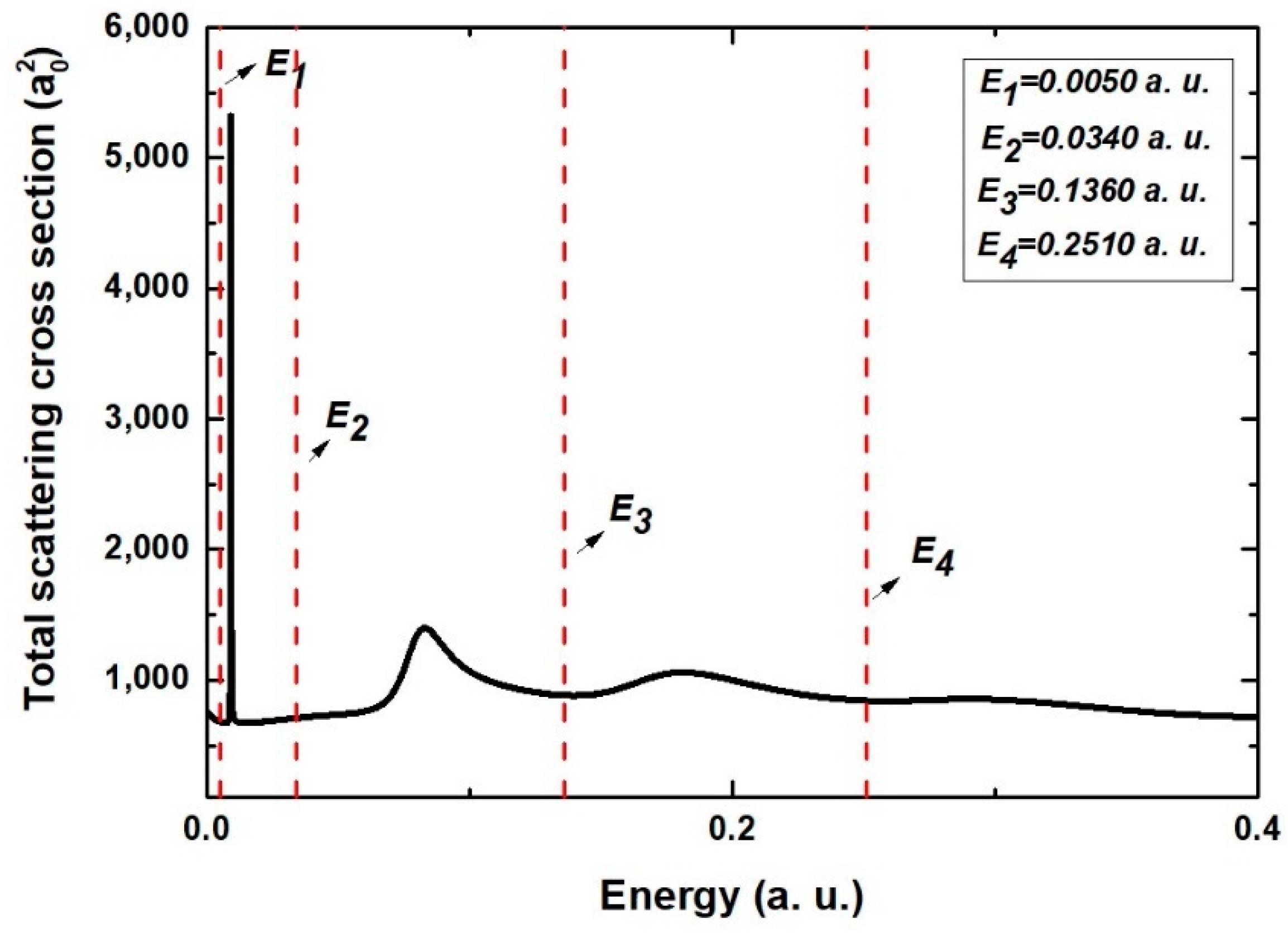
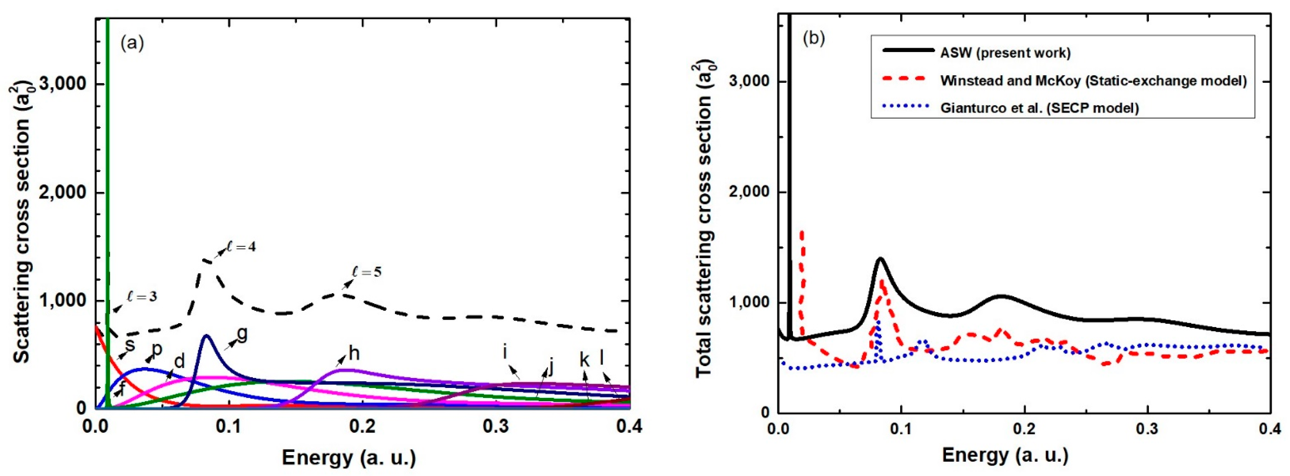
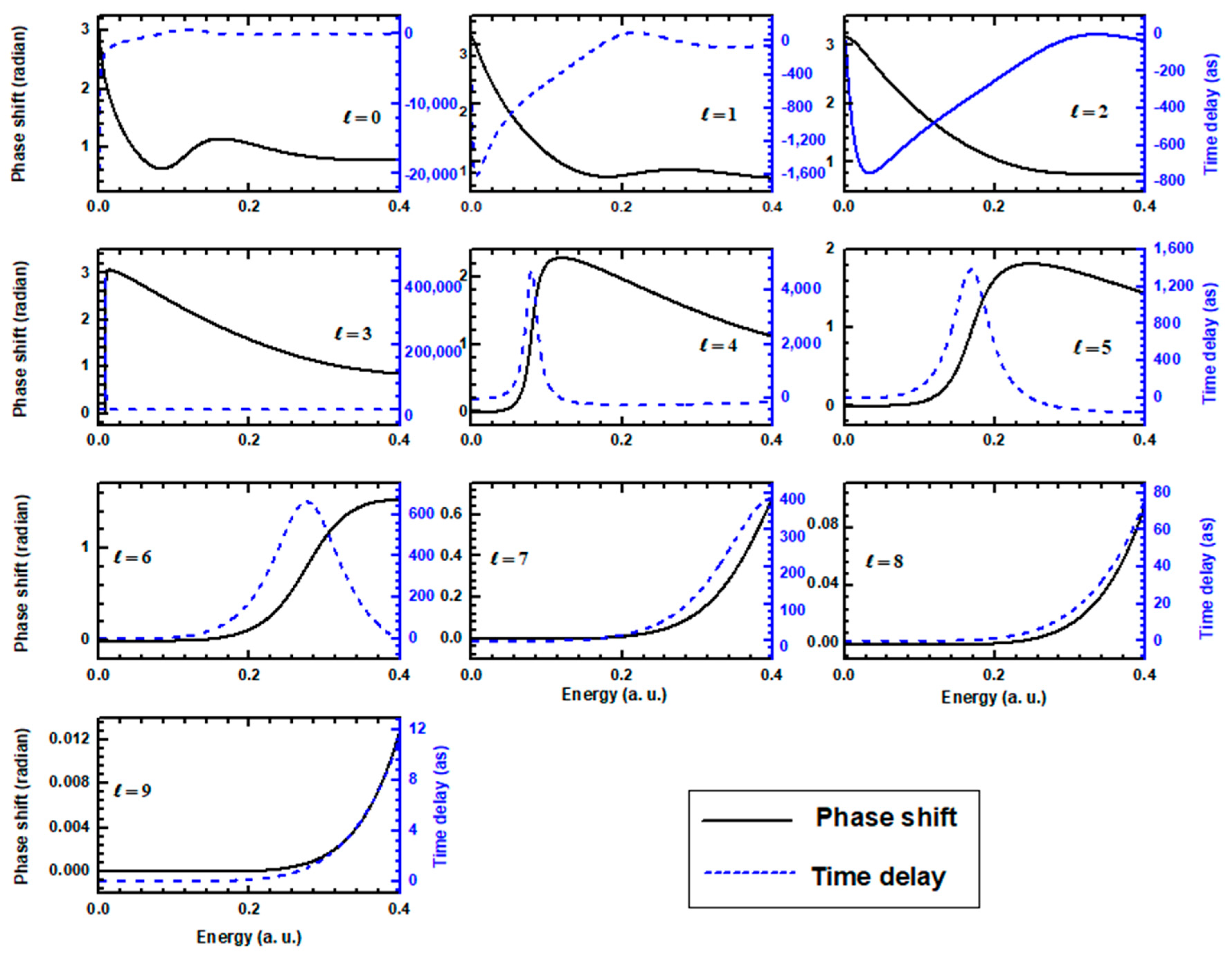
3.1. TCS, PCS, and EWS Time Delays

Figure 1a shows the total and the partial cross-sections of the e-C60 elastic scattering contributed by = 0   to   9 partial waves. The higher partial waves beyond = 9 did not contribute to the low-energy scattering, and hence they were not accounted for in the calculation.
In Figure 1a, it can be noted that the total scattering cross-section consists of three peaks, which indicate the resonances in the elastic scattering. The PCS analysis showed that partial waves with angular momentum quantum numbers = 3 , 4   and   5 were resonantly scattered with the corresponding resonant energies Er = 0.0091, 0.0829, and 0.1811 a.u., respectively. Among the three peaks, the = 3 partial wave resonance was the sharpest, and that of = 5 was the weakest among the three. The = 6 partial wave also exhibited a much weaker resonance at 0.2907 a.u., which was noticeable as a relatively smaller hump in the total cross-section. These observations using the ASW model of the C60 were quite consistent with earlier calculations [67,77,78].
Before proceeding, a comparison of the total scattering cross section from the present calculation with other molecular level theories [63,64] is presented in Figure 1b. Winstead and McKoy [64] calculated the integral cross-section using the static-exchange model, whereas Gianturco et al. [63] used a theory that included the impact of polarisation additionally, termed as the static-exchange core polarization (SECP) model. The present spherical ASW approximation rendered a good qualitative comparison in terms of the prominent resonances. However, the higher-level theories showcased a greater number of molecular resonances that could not be represented by a spherical potential approximation. Although the quantitative agreement was missing, the qualitative comparison encouraged the use of the simple but robust ASW model for the scattering calculations.
To further demonstrate the efficiency of ASW potential, DCS was plotted (Figure 2) for energies (2 eV, 4 eV, 7 eV, and 10 eV), and the results were compared with ab initio theoretical [63,64] and experimental results [17]. The experimental results of Tanaka et al. [17] were only available for the incident energies (4 eV, 7 eV, and 10 eV). The DCS showed the number of diffraction-type minima, which increased as the scattering energy was increased. This behaviour was due to the enhanced contribution from higher partial waves at increased energies. Further, we found that the DCS from the present ASW calculation agreed well with the measurements and lay within the uncertainties of most of the data points. Qualitative and quantitative agreement of the present result with the ab initio theories was also commendable. The agreement encouraged us to further employ the ASW parameters for the time delay calculations.
The EWS time delay is a fundamental quantity in the scattering formulation that reflects the temporal features of the resonant electron, such as how long a projectile electron is trapped in the quasi-bound state formed by the projectile–target interaction. In Figure 3, the scattering phase shift and EWS time delay (using Equation (6)) are plotted for partial waves = 0 9 . In accordance with the Wigner threshold law, the s-wave phase shift in the limit k 0 tended to the value π and it reduced as ( π E ) from the threshold [79]. Hence, the time delay for the s-wave exhibited a large negative value; δ 0 ( E 0 )   tends   to   E 1 / 2 . The non-zero angular momentum partial waves exhibited zero-time delay at the threshold, which also followed the Wigner threshold law.
It is well known that at the resonance, the scattering phase shift goes through a π / 2 , and across the resonance, it changes by the value π [76]. In unison with this, for partial waves = 3 , 4   and   5 , a sharp jump in the phase shift was observed at the corresponding resonant energy. Consequently, the resonant time delay was larger; the stronger resonance of the = 3 partial wave caused a larger time delay of 423,832.29 as at the resonance, and the weaker resonance of the = 5 partial wave resulted in a relatively smaller time delay of 1395.52 as. A general trend was that the non-resonant time delays were relatively smaller than those corresponding to the resonant scattering. In Equation (13), one can see that the EWS time delay ( δ ) of a particular partial wave contributes to the numerator when the pair terms are summed. Due to this reason, it was expected that the resonant channels would show their dominance even in the angular time delay; this will be examined in the next section. Regarding the resonance, it was expected that the partial waves would play their role depending on the strength of the scattering. For instance, the angular time delay near the threshold would have dominance due to the s-wave scattering. The further sections discuss the resonant and the non-resonant angular time delay in the e-C60 elastic scattering.

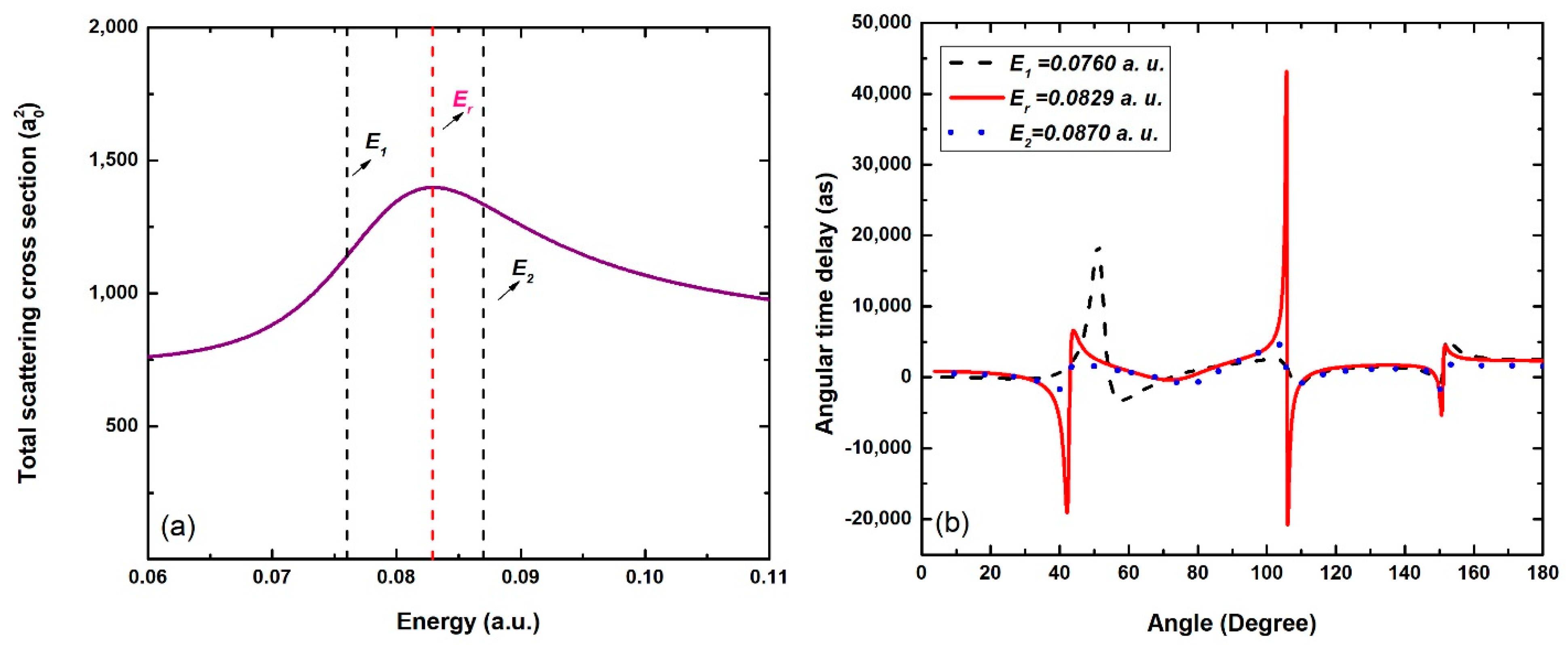
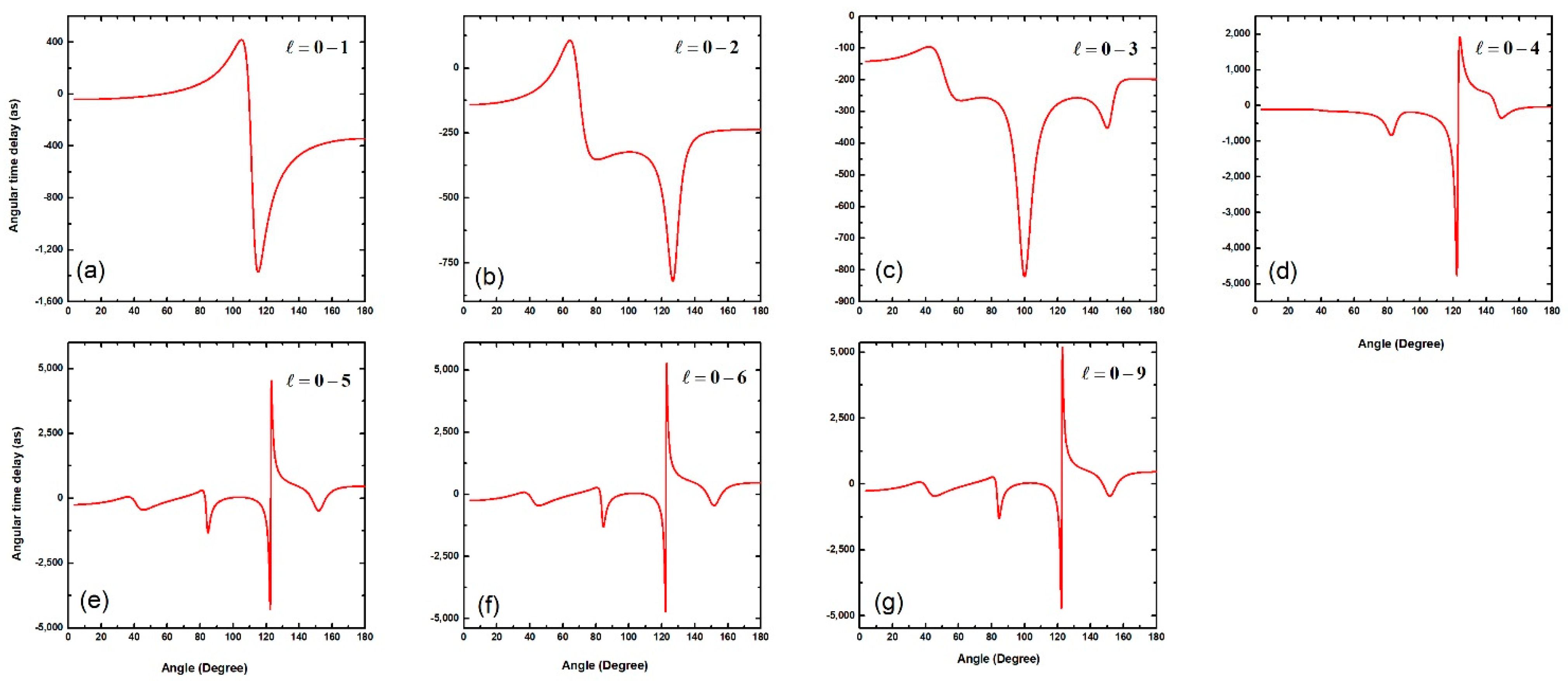
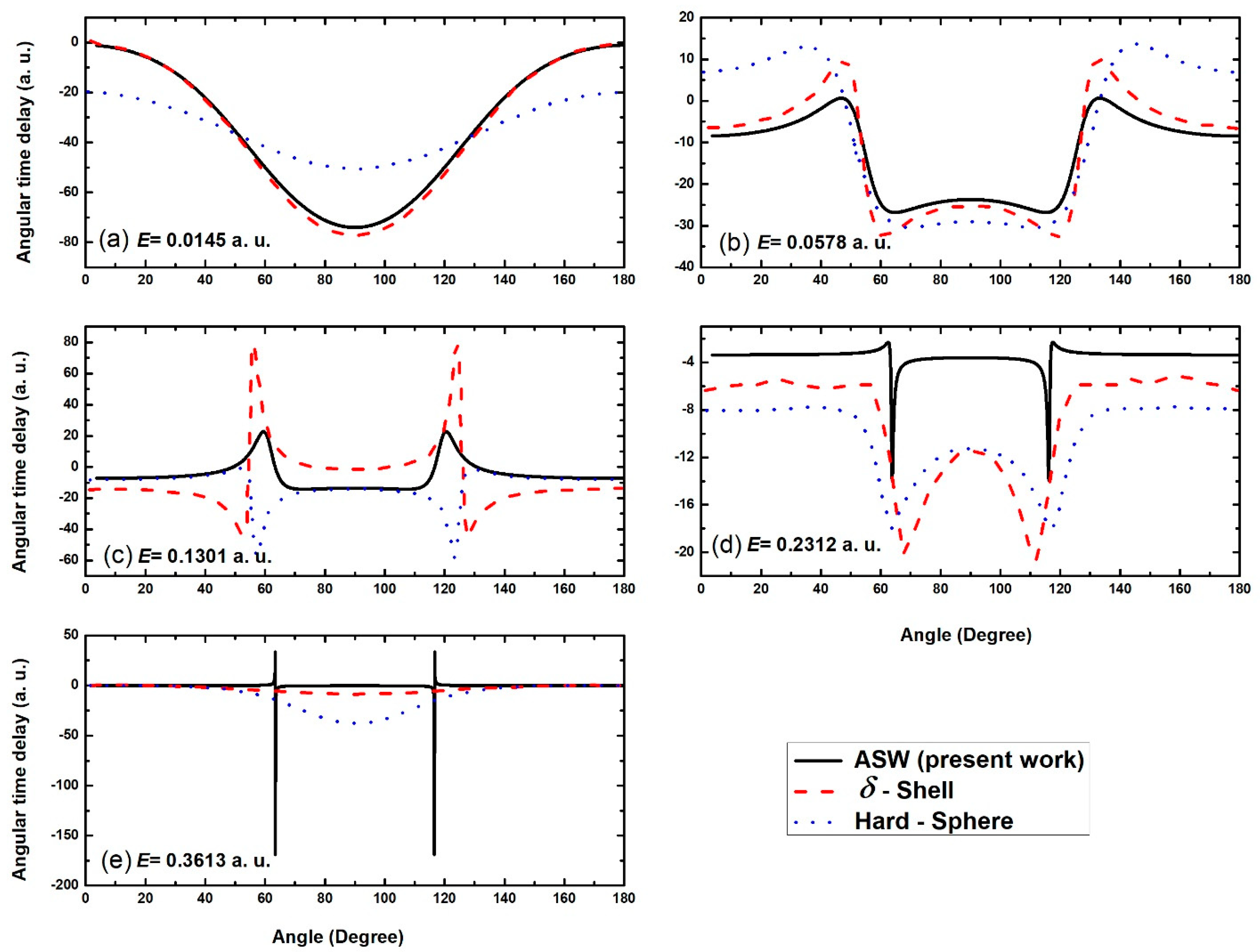
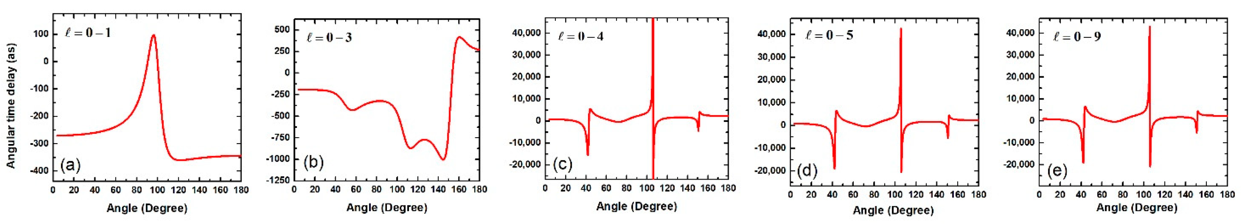
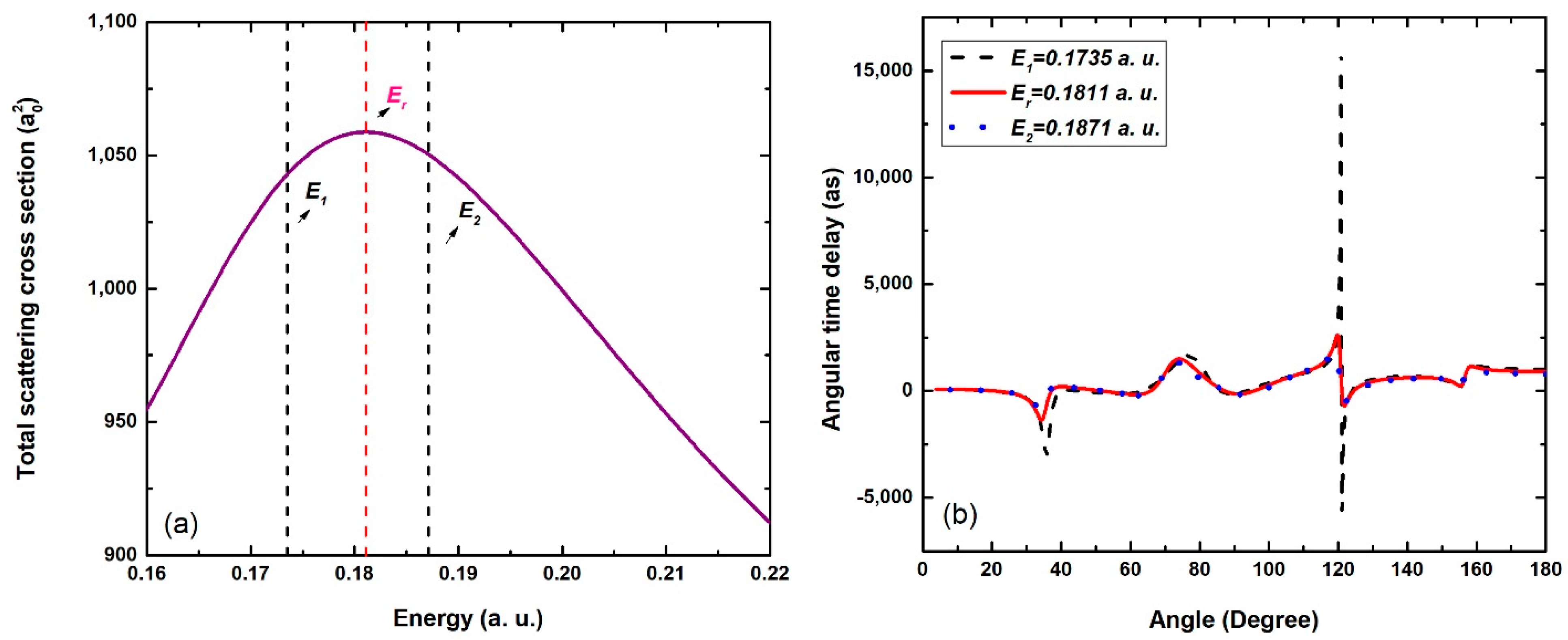
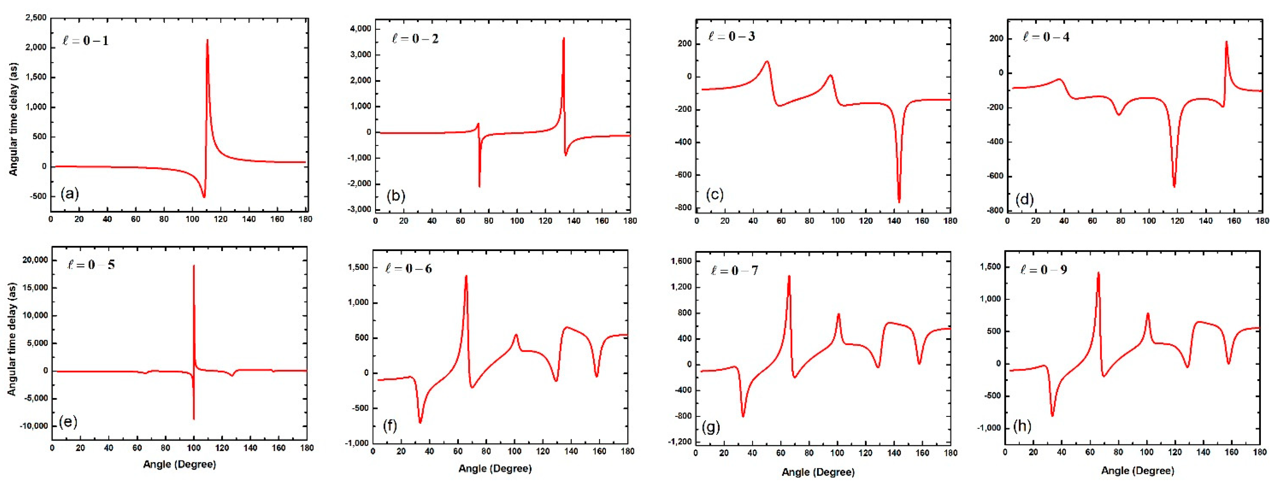
3.2. Resonant Angular Time Delay
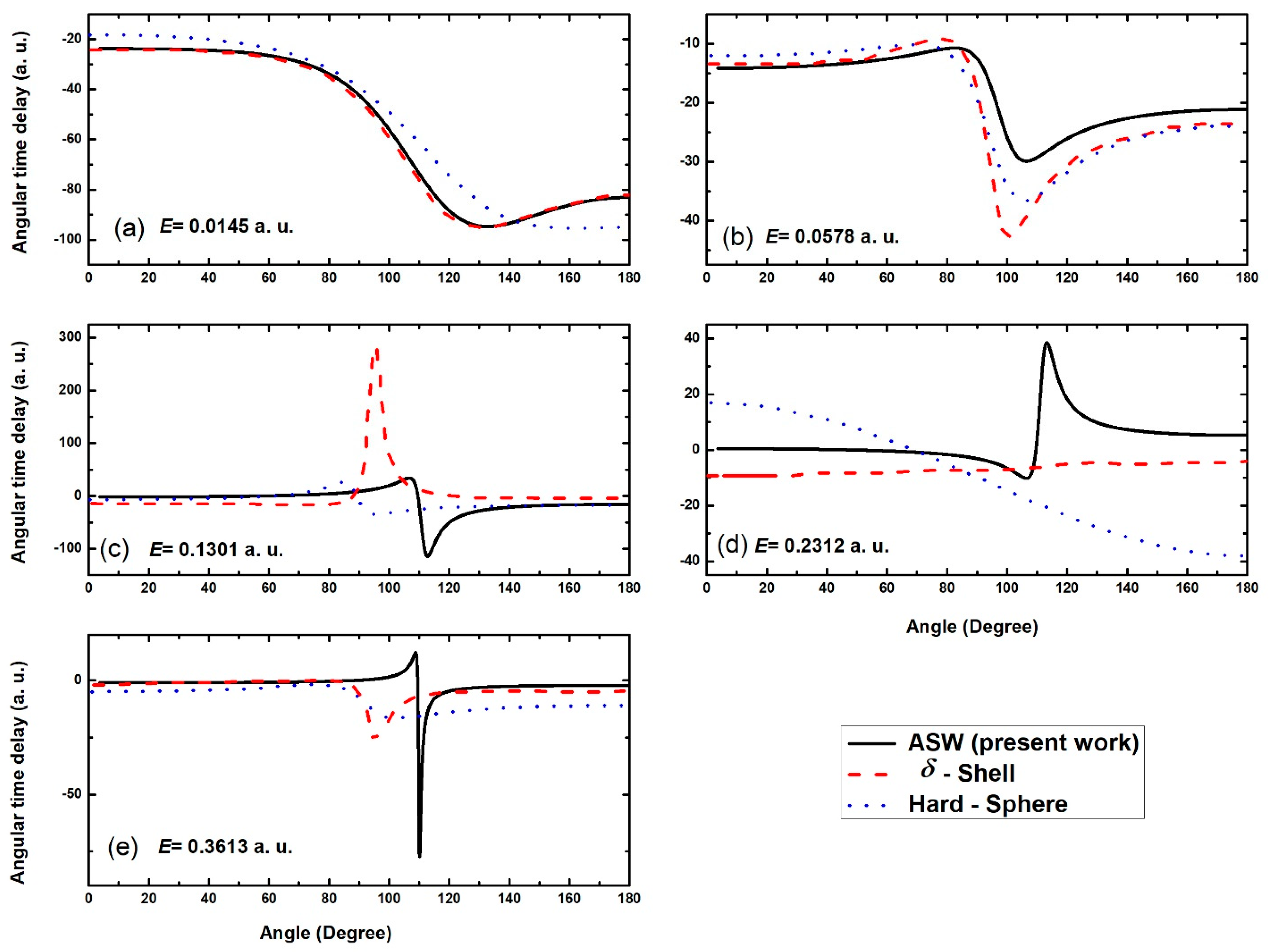
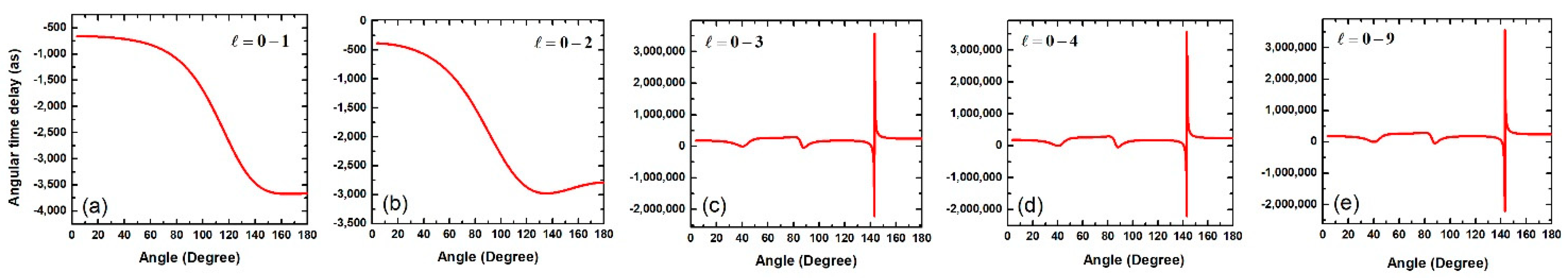
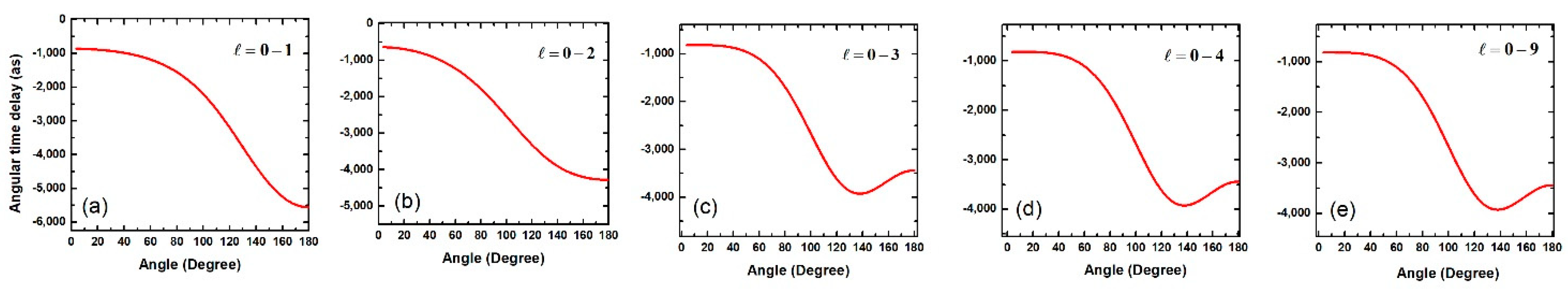
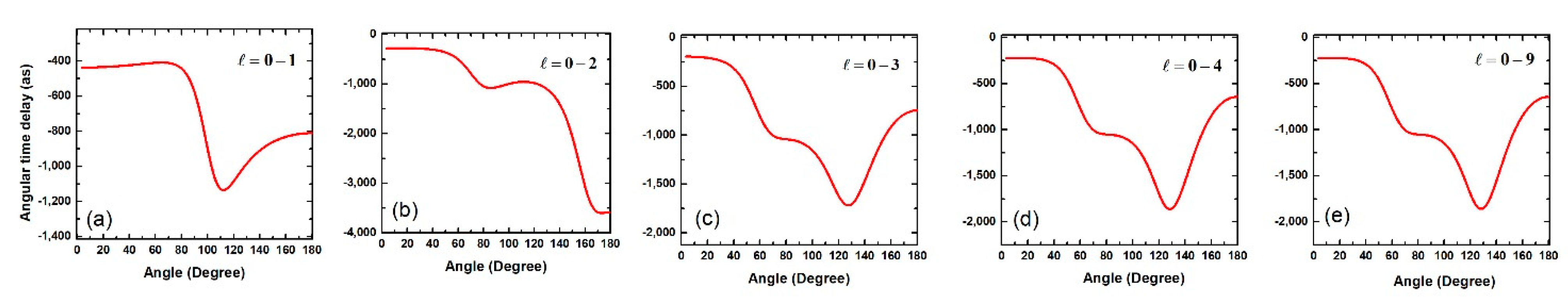
 ( Δ t ( k , θ ) )

As seen in Figure 1a, three prominent resonances were in the elastic TCS of the e-C60 collision; the = 3 partial wave was resonant at Er = 0.0091 a.u., = 4 at Er = 0.0829 a.u., and = 5 at Er = 0.1811 a.u. The present section successively analyses the angular time delay at these resonant energies. Further, an evolution of the angular time delay when the projectile energy is varied across a resonance is also investigated.
As detailed in Section 2, the angular time delay is a consequence of the interference of the partial waves. From Equation (13), one can understand that the summation in the numerator and the denominator can be truncated to analyse the contribution of each partial wave in the angular time delay. In other words, the dominance of interference of the particular partial waves, say 1 , and 2 , can be examined by restricting the and in Equation (13) to run for only 1 and 2 . The Δ t 1 , 2 ( k , θ ) for the 1 and 2 interference case is expressed as:
Δ t 1 , 2 ( k , θ ) = [ ( 2 1 + 1 ) 2 P 1 2 sin 2 δ 1 + ( 2 1 + 1 ) ( 2 2 + 1 ) P 1 P 2 sin ( 2 δ 1 δ 2 ) sin δ 2 ] δ 1 + [ ( 2 2 + 1 ) 2 P 2 2 sin 2 δ 2 + ( 2 1 + 1 ) ( 2 2 + 1 ) P 1 P 2 sin ( 2 δ 2 δ 1 ) sin δ 1 ] δ 2 ( 2 1 + 1 ) 2 P 1 2 sin 2 δ 1 + ( 2 2 + 1 ) 2 P 2 2 sin 2 δ 2 + 2 ( 2 1 + 1 ) ( 2 2 + 1 ) P 1 P 2 sin δ 1 sin δ 2 cos ( δ 1 δ 2 )
In a similar fashion, by keeping suitable values of angular momentum quantum numbers for the and in the summation in Equation (13), the additional contribution of each partial waves in the anisotropic time delay can be investigated. This procedure was adopted in the present work to examine the resonant scattering.
Before examining the ASW resonant time delay, a comparison of the present results with those of the recent works of Amusia et al. [50] is outlined below.
A comparison of the angular time delay for partial wave combination = 0 , 1 (Figure 4) and = 0 , 2 (Figure 5) using the ASW potential, δ-shell [50], and hard sphere [50] was made. For lower energies, in Figure 4a,b, it can be noted that there is a good agreement between the present ASW results and those of Amusia et al. [50]. The Δ t 0 , 1 ( k , θ ) varied smoothly from a lower negative time delay to a higher one. Since the s-wave scattering dominated the lower-energy collision, all three potentials rendered similar angular time delay profiles. Not only that, the Wigner threshold law held a similar partial cross-section in all three potential cases, which also ensured a similar Δ t 0 , 1 ( k , θ ) . The same goes for partial wave combination = 0 , 2 (Figure 5a,b); Δ t 0 , 2 ( k , θ ) , which also maintained a similar profile for all three model potentials in the low energies. As the energy increased, there was a marked deviation in the angular time delay, Δ t 0 , 1 ( k , θ ) and Δ t 0 , 2 ( k , θ ) , between the three different models. This was due to the fact that the non-resonant scattering cross-section was different in different model potential cases. Next, we examined the resonant angular time delay in the ASW case.
Er = 0.0091 a.u.
Figure 6 shows the angular time delay at the resonant energy Er = 0.0091 a.u., which corresponded to the = 3 resonance. Figure 6a shows the interference pattern in Δ t 0 , 1 ( k , θ ) due to the = 0 and 1 partial waves. The entire time delay was negative; the Δ t 0 , 1 ( k , θ ) varied smoothly from ~−700 as to −3750 as when the angle is varied from forward to backward scattering directions. The time advancement (negative time delay) was consequent to the negative values of the EWS time delay, ( δ 0 = 1332.70   as , δ 1 = 790.44   as ) at the Er = 0.0091 a.u. Figure 6b includes the interference effects due to = 2 in addition to the first two. One can see that there was not much appreciable change in the profile of the angular time delay, except a minor quantitative change; Δ t 0 2 ( k , θ ) varied from ~−500 as to ~−3000 as when the scattering angle was altered. Here also, the Δ t 0 2 ( k , θ ) lay in the negative region, as the EWS time delay contribution from the partial wave = 2 was also negative ( δ 2 = 216.74   as at Er = 0.0091 a.u.). Note that δ 2 also was small compared to that of the other partial waves included. A striking change in the angular time delay profile ( Δ t 0 3 ( k , θ ) ) was seen upon adding the resonant partial wave = 3 , which is evident in Figure 6c. The Δ t 0 3 ( k , θ ) was positive for most of the angles. However, the delay crossed zero and became negative in the vicinity of angles ~40.28° and ~88.16°.
At 143.22°, a sharp jump from a positive to negative infinite value in the time delay was observed. Further, at ~144.09°, the time delay value increased rapidly and finally tended to a large positive value. Note that the Δ t 0 , 1 ( k , θ ) and Δ t 0 2 ( k , θ ) were negligibly small compared to the overall magnitude of the angular time delay upon the addition of the effects of the resonant partial wave. Therefore, we can say that the resonant angular time delay profile was mostly governed by the corresponding resonant partial wave.
The angular dependence of the resonant time delay ( Δ t 0 3 ( k , θ ) ) was further explained with the help of Equation (13). Term-wise analysis of the numerator and the denominator revealed that the interaction of the = 3 partial wave with those having = 0 , 1 , 2 , 3 was more dominant than the interactions due to other combinations of ( , ) values. This was because the δ 3 was the resonant EWS time delay, which was quite large (~213,352 as) at the resonant energy Er = 0.0091 a.u. The large positive resonant time delay controlled the fate of the angular time delay at the Er and consequently, terms with = 3 and = 0 , 1 , 2 , 3 in the summation in Equation (13) were weighted by the large δ 3 . This means that the approximated Δ t 0 3 ( k , θ ) at the resonant energy Er = 0.0091 a.u. is written as:
Δ t 0 3 ( k , θ ) = 0 , 1 , 2 , 3 [ 7 ( 2 + 1 ) P 3 P sin ( 2 δ 3 δ ) sin δ ] δ 3 = 0 , 1 , 2 , 3 7 ( 2 + 1 ) P 3 P sin δ 3 sin δ cos ( δ 3 δ )
The numerator of Δ t 0 3 ( k , θ ) (Equation (15)) was mostly positive and obtained minimum values at angles 39.26°, 89.99°, and 140.75°, which was due to the zero-crossing of the Legendre polynomial P 3 ( cos θ ) at these angles. However, upon further addition of coupling terms to it, these minima became further widened and deeper, resulting in the shallow dips at ~40.28° and ~88.16° in the angular time delay Δ t 0 3 ( k , θ ) . The explanation behind the large positive and negative values at angle ~144° was sought next. An analysis of the denominator of Δ t 0 3 ( k , θ ) showed that it also had three minima almost coincided at the minimum angles of the numerator. However, the value of the minimum of the denominator at angle 143.22° was very small (almost zero) compared to the numerator, which led to an enhanced angular time delay at ~144 degrees. Thus, the profile of the resonant angular time delay was explained when = 0 , 1 , 2   and   3 partial waves were coupled. However, note that other partial waves were also contributing through non-resonant scattering; their interference effect on the angular time delay is elucidated next.
Figure 6d shows Δ t 0 4 ( k , θ ) when the partial waves with angular momenta , = 0 , 1 , 2 , 3   and   4 were included in Equation (13). It is of no surprise that the addition of = 4 partial wave at energy Er = 0.0090 a.u. did not impart any change in the angular time delay. This means that the = 3 dominance prevailed due to the resonant scattering. Further, we included all contributing partial waves = 0 9 , and the result of the angular time delay Δ t 0 9 ( k , θ ) is shown in Figure 6e. One can see that the profile remained the same as in Figure 6c. Thus, the resonant angular time delay at Er = 0.0090 a.u. was examined, and the analysis showed that the resonant channel dominated the anisotropy. The symmetry of P 3 ( cos θ ) controlled the angular time delay significantly.
The earlier analysis showcased the prominence of the = 3 partial wave in contributing to the resonant angular time delay. Next, we analysed the evolution of the angular time delay across the first resonance. For that, we chose two energy points: E1 = 0.0089 a.u., below the Er; and E2 = 0.0093 a.u., above the resonance. Figure 7a shows the total cross-section near the = 3 resonance, and the vertical line indicates the energy points E1 and E2 we chose for the analysis, in addition to the resonant energy Er. Figure 7b shows the evolution of the angular time delay as the projectile energy varied across the resonance from E1 to E2 through the Er. The effective angular time delay was plotted by including the interference of all the contributing partial waves; i.e., Δ t 0 9 ( k , θ ) in this case.
Figure 7b thus shows the evolution of the angular time delay across the first resonance. It can be understood that the zero crossings of the angular time delay were similar for the three energies, which was indicative of the dominance of the = 3 partial wave through the P 3 ( cos θ ) .
The profile of Δ t 0 9 ( k , θ ) at E1 showed that the angular time delay value was negative for smaller angles, with a minimum at 22.33°. The negative time delay value gradually decreased, and at 39.38°, its value crossed zero and tended further to a positive value. The time delay value maintained a plateau region between the angles 50° and 80°, beyond which it began decreasing and crossed zero to a negative value at 89.83°. Two minima in negative time delay values were observed for the angles 97.99° and 135.81°. Again at 141.08°, the time delay value crossed zero to a positive value and remained in the positive range, with a peak at 149.65°. The truncated partial wave analysis showed that, even for off-resonant energy at E1 = 0.0089 a.u., = 3 was the most dominant channel contributing to the angular time delay. Due to this, the P 3 ( cos θ ) governed the zero crossings of the Δ t 0 9 ( k , θ ) . The Legendre polynomial, P 3 ( cos θ ) , had zero-crossings at the angles 39.29°, 89.99°, and 140.76°. The coupling with other partial waves caused the zero-crossing point of Δ t 0 9 ( k , θ ) at E1 to slightly shift to the angles 39.31°, 89.80°, and 140.99°.
The entire nature of angular time delay at E1 was controlled by the interaction between partial waves with = 3 and those with = 0 , 1 , 2 , 3 . The contribution from higher values to the angular time delay part was almost negligible, as seen in our analysis. Unlike in the resonant case, among the pair terms in the numerator, = 3 , = 0 coupling was stronger at E1. The angular time delay at the E1 is, therefore, approximately written as:
Δ t 0 9 ( k , θ ) [ P 3 2 sin 2 δ 3   +   7 P 3 P 0 sin ( 2 δ 3     δ 0 ) sin δ 0 ] δ 3   +   [ 49 P 0 2 sin 2 δ 0   +   7 P 3 P 0 sin ( 2 δ 0     δ 3 ) sin δ 3 ] δ 0 P 3 2 sin 2 δ 3   +   49 P 0 2 sin 2 δ 0   +   14 P 3 P 0 sin δ 3 sin δ 0 cos ( δ 3     δ 0 ) .
Note that the terms with = 3 and = 0 , 1 , 2 , 3 were the flag bearers in the resonant case, but in the off-resonant case, coupling of = 3 with = 0 dominated. We saw that this shift in the importance at E1 was due to the prominence of s-wave scattering for low energies. A strange combination of the resonant and the non-resonant channels was evident here.
For the off-resonant state energy at E2 = 0.0089 a.u., = 3 also was the most prominent factor that contributed to the angular time delay, Δ t 0 9 ( k , θ ) . The qualitative behaviour of the angular time delay was controlled by the partial wave = 3 . In Figure 7b, it can be observed that angular time delay was positive for most of the angles. Three small negative dips in the time delay values were observed at the angles 42.86°, 93.55°, and 137.64°. In addition, two positive peaks were observed; one larger peak was at 57.72°, and a smaller one was at 148.54°. The zero-crossing of the angular time delay was governed by the symmetry of the P 3 ( cos θ ) .
Er = 0.0829 a.u.
As evident in Figure 1a, at energy Er = 0.0829 a.u., the = 4 partial wave underwent a resonant scattering. Motivated by the earlier discussion, it was intuitive that the resonant = 4 partial wave would be dominant in the angular time delay at the energy Er = 0.0829 a.u. To investigate this, Figure 8 shows the angular time delay at Er = 0.0829 a.u. after including interference in a truncated manner. Figure 8a shows the angular time delay, Δ t 0 , 1 ( k , θ ) , after including the coupling of only the s- and p-waves. The time delay value lay in the negative range for most of the angles. A zero-crossing in the time delay value was observed at the angles 90.63° and 100°, with a small positive peak at 96.14°. The overall value of the Δ t 0 , 1 ( k , θ ) ranged between ~−350 as and 100 as. With the further addition of the d-wave, the time delay profile remained in the negative region throughout. The entire profile lay in between ~−250 as to −950 as, and had two dips at 72.14° and 140.52°. In a step-wise manner, Figure 8b additionally includes the impact of the = 3 partial wave and shows Δ t 0 3 ( k , θ ) . Here also, the time delay value was negative for most of the angles, and it crossed over to the positive region at 153.76°. The Δ t 0 3 ( k , θ ) had three dips at the angles 56.29°, 113.12°, and 144.68°. Although the Δ t 0 3 ( k , θ ) profile was qualitatively different compared to the previously truncated results, Δ t 0 , 1 ( k , θ ) and Δ t 0 2 ( k , θ ) , the overall range of the time delay was not dramatically different compared to theirs. Figure 8c incorporates the interference due to = 4 and shows the Δ t 0 4 ( k , θ ) . A remarkable difference in the angular time delay profile was noted qualitatively and quantitatively upon the inclusion of = 4 partial waves; the range of Δ t 0 4 ( k , θ ) varied from ~40,000 as to ~−20,000 as. The Δ t 0 4 ( k , θ ) had zero-crossings at the angles 28.90°, 43.01°, 66.32°, 76.95°, 105.86°, 111.04°, 149.16°, and 150.44°. Additionally, the time delay increased on one side and suddenly changed sign and grew to a peak at the angles 41.93° and 150.69°. After the small dip at 150.69°, the time delay value remained at an almost flat positive constant. A dramatic change in the time delay was noted in the vicinity of θ 106 0 . Its value crossed over to a negative time delay value at angle 111.04°, after which it decreased rapidly and finally tended to negative infinity. At 105.86°, a sharp jump from a negative to positive infinite value in the time delay was observed. Upon analysing terms present in Equation (13), it was seen that the interaction term due to = 4 and = 0 , 1 , 2 , 3 , 4 was the most dominant. The most significant term in the numerator was that with = 4 and = 4 : [ 81 P 4 2 sin 2 δ 4 ] δ 4 with δ 4 = 2110.57   as , which was the resonant EWS time delay. Note that the resonant time delay was larger than the non-resonant ones at the particular energy. Thus, the resonant channel governed the angular time delay profile. For more clarity, it can be noted that the zero-crossings of the angular time delays were in the near vicinity of the nodes of the Legendre polynomial P 4 ( cos θ ) . The relative weightage of the numerator and the denominator terms with = = 4 controlled the shape of the total angular time delay profile. To further examine the impact of the higher angular momentum partial waves, terms corresponding to = 5 were also added; Δ t 0 5 ( k , θ ) is shown in Figure 8d. Note that the qualitative nature of the Δ t 0 5 ( k , θ ) was no different compared to the predecessor’s profile. Further, all contributing partial waves were added ( Δ t 0 9 ( k , θ ) ) and are displayed in Figure 8e. It was not a surprise that the profile of the angular time delay remained the same as in the case when the resonant channel was added. This indicated that at the resonance, the resonant partial wave dominated the angular time delay.
Next, the evolution of the angular dependence of the time delay was investigated at the non-resonant energies, but close to the Er. Figure 9a shows the total scattering cross-section near the resonance of the = 4 partial wave, and the vertical lines indicate the energy points at which the time delay was examined; E1 = 0.0760 a.u. was lower than the resonant energy, and the E2 = 0.0870 a.u. was higher than the Er. The angular time delay is plotted for E1, E2, and Er in Figure 9b. Contributions from all the partial waves, = 0 9 , were incorporated to visualise the realistic interference impact on Δ t 0 9 ( k , θ ) .
Our analysis showed that the partial wave with = 4 was the most vital one contributing to the angular time delay for the off-resonant state energy at E1 = 0.0760 a.u. The contribution from higher partial waves was almost negligible. We observed that the time delay value was positive for most of the angles with three minima, with negative time delays at 57.72°, 108.96°, and 150.23°. Large positive time delays were noted at 51.02° and 152.37°. For smaller angles, the time delay values remained almost constant and were small. The time delay profile had multiple zero-crossing points, which were at 10.62°, 35.52°, 54.370, 72.26°, 106.99°, 112.42°, 148.29°, and 150.75°. Among the numerator terms in Equation (13), the interaction of the = 4 partial wave and those with = 0 , 1 , 2 , 3 , 4 were more dominant than the interactions due to other combinations of partial waves. Here again, the most prominent contributing factor in the numerator was due to the term with = = 4 , which is [ 81 P 4 2 sin 2 δ 4 ] δ 4 ; the value of δ 4 = 2079.13   as at E1 was large compared to other partial waves’ EWS time delays. This term in the numerator had sharp dips (almost zero) at the angles 30.57°, 70.12°, 109.87°, and 149.41°. This was due to the zero-crossing nature of the Legendre polynomial P 4 ( cos θ ) through these angles. However, further addition of coupling terms to it caused these dips to shift. The final profile of the numerator term had minima at the angles 22.93°, 64.34°,109.75°, and 149.54°. Note that these dips had a straightforward connection with the zero-crossing in the Δ t 0 9 ( k , θ ) . Coming to the enhanced time delay at 51.09°, upon analysing the denominator expression of Δ t 0 9 ( k , θ ) , it was again observed that the = 4 contribution dominated there as well. When a minimum was present in the denominator expression of Δ t 0 9 ( k , θ ) , the angular time delay had a higher value. Since the nodes in P 4 ( cos θ ) governed the profile, associated with the zeros in the Legendre polynomial, a maximum in the time delay was also seen.
Regarding the Δ t 0 9 ( k , θ ) at E2 = 0.0870 a.u., the partial wave with = 4 was the most vital one that contributed to the angular time delay for this off-resonant energy as well. The contribution from higher partial waves was almost negligible. We observed that the time delay value was positive for most of the angles. However, the Δ t 0 9 ( k , θ ) exhibited three minima, with negative time delays at 57.72°, 108.96°, and 150.23°. Large positive time delays were noted at 51.02° and 152.37°. For smaller angles, the time delay values remained almost constant and were small. At the angles 28.20°, 41.80°, 67.46°, 82.90°, 106.28°, 113.39°, 148.79°, and 150.94°, zero-crossings in Δ t 0 9 ( k , θ ) were observed. Following the analysis of E1, the = 4 partial wave dominated the Δ t 0 9 ( k , θ ) at E2 = 0.0870 a.u. as well. Since the EWS time delay at E2 was larger ( δ 4 = 1443.65   as ) compared to that of the other partial waves, P 4 ( cos θ ) governed the nodal points and the enhanced time delays.
Er = 0.1811 a.u.
In this subsection, angular time delay at the resonant scattering corresponding to the = 5 partial wave at Er = 0.1811 a.u. is considered. Figure 10a presents the Δ t 0 , 1 ( k , θ ) due to the interference between = 0 and 1 at Er = 0.1811 a.u. The profile of Δ t 0 , 1 ( k , θ ) had a dip at 104.41° and a small peak at 123.80°, along with a zero-crossing at 114.05°. The addition of four more partial waves ( = 1 , = 2 , = 3 , and = 4 ) gave rise to the dramatic angular distribution of the time delay, as shown in Figure 10b. Note that these partial waves were non-resonant at these energies. The time delay Δ t 0 4 ( k , θ ) had negative values, with minima at the angles 79.76°, 122.22°, and 149.22°. The addition of the resonant channel ( = 5 ) significantly modified the qualitative profile; more positive peaks appeared in Δ t 0 5 ( k , θ ) , as shown in Figure 10c. The magnitude of the time delay was altered upon the addition of the resonant channel; the Δ t 0 5 ( k , θ ) varied from −1000 as to 4000 as. However, the change was not as dramatic as upon the addition of resonant channels at Er = 0.0829 a.u. and Er = 0.0091 a.u. This was because the = 5 partial wave showed only a weak resonance at Er = 0.1811 a.u. The weightage of the interaction of = 5 with other partial waves was relatively less due to δ 5 = 579 . 11   as , which was diminutive compared to δ 3 and δ 4 at the respective resonances.
Similar to earlier cases, here also the contribution from higher partial waves was almost negligible, as evident in Figure 10d,e. We noted that angular time delay, Δ t 0 5 ( k , θ ) , took both positive and negative values, with a deeper negative dip at 34° and two smaller dips at the angles 62.22° and 91.14°. In addition, we observed a large positive peak at the angle 73.56° and a smaller one at 40.54°. After passing through the small dip at 91.14°, the time delay value gradually increased and tended to positive infinity. Later, a jump from a positive to a negative time delay value was observed at the angle 121.39°. A negative time delay value was observed until the angle 124.12°, above which the Δ t 0 5 ( k , θ ) was observed to be positive, with a small positive dip at 155.50° and a small positive peak at 158.12°. We noted that although the interference effects with = 5 significantly modified the angular anisotropy, the back-scattering time delay was also governed by partial waves with the angular momentum quantum numbers = 0 , 1 , 2 , 3   and   4 , which were all non-resonant (see Figure 10c). This was due to the fact that the = 5 resonance was relatively weaker, and the non-resonant channels also actively took part in the interference among themselves.
Our analysis showed that the interaction between the = 5 partial wave and those with = 0 , 1 , 2 , 3 , 4 , 5 was the dominant one that caused the angular profile of the time delay. Among the terms in the numerator of Δ t 0 5 ( k , θ ) , contributions from the term [ 121 P 5 2 sin 2 δ 5 ] δ 5 , corresponding to = = 5 with δ 5 = 578 . 87   as , were relatively prominent. This component had a sharp dip at the angles 25.03°, 57.45°, 90°, 122.54°, and 154.94°; in the vicinity of these angles, the angular time delay crossed zero. The reason was the zero-crossing nature of the Legendre polynomial P 5 ( cos θ ) through these angles. With further contributions from interacting partial waves, the final profile of the numerator term had minima at the angles 27.13°, 58.59°, 91.37°, 122.75°, and 155.64°, with the minimum at 27.13° being the deepest among the five.
Further examination clarified that the denominator of Δ t 0 5 ( k , θ ) had three minima, at the angles 35.11°, 121.26°, and 156.49°. An analysis of the terms present in the denominator of the time delay pinpointed that the term [ 121 P 5 2 sin 2 δ 5 ] δ 5 was the most dominant one. Note that corresponding to these minima, the angular time delay was enhanced.
Similar to the earlier cases, we extended the examination to the off-resonant energies, but near the Er = 0.1811 a.u. Figure 11a shows the total scattering cross-section near the = 5 partial wave resonance and the non-resonant energies under consideration (E1 = 0.1735 a.u., E2 = 0.1871 a.u.); the Er are marked with vertical lines. Figure 11b shows the development of the angular time delay, Δ t 0 9 ( k , θ ) , as the projectile energy was scanned across the resonance.
Since the E1 = 0.1735 a.u. was close to the resonance, we expected that the = 5 partial wave would govern the angular distribution of the time delay, and that the zero-crossing of the time delay would be mostly in the vicinity of nodes in the P 5 ( cos θ ) . The Δ t 0 9 ( k , θ ) took both positive and negative values, with a deeper negative dip at 35.51° and two smaller dips at the angles 58.06° and 89.08°. In addition, we observed a large positive peak at the angle 76.29°. After passing through the small dip at 89.08°, the time delay value gradually increased and tended to positive infinity. Later, a jump from a positive to a negative time delay value was observed at the angle 121.40°. The reason for the time delay being infinite in this range was the fact that the magnitude of the denominator in Equation (13) was far smaller than the numerator. Although the prominent contribution was from the = 5 partial waves, the non-resonant channels also interfered in the back-scattered angles, resulting in a significant time delay. This was due to the weaker nature of the = 5 resonance.
At the off-resonant energy E2 = 0.1735 a.u., the contribution of the = 5 term was weighted almost as equally as the other lower partial waves, which were non-resonant. Our truncated analysis showed that the interference of the = 0 , 1 , 2 , 3 , and 4 partial waves led to several dips in the angular profile of the time delay, in particular in the back-scattered region. Upon adding the coupling with = 5 , more structures were created due to the resonances. However, since the resonance was weak, the other channels also contributed.

3.3. Angular Time Delay, Δ t ( k , θ ) , at Far-Off Resonant Energies

Section 3.2 analysed the angular anisotropy of the time delay at the resonant energies and the non-resonant energies in the vicinity of the resonances. We concluded that the time delay in the resonance region was contributed significantly by the interference effects of the resonant partial waves. Now we will examine the angular time delay in the far-off resonant region, where we expected contributions from all the significant partial waves depending on their background cross-section. Figure 12 shows the total cross-section; the off-resonant energy points under the investigation are marked with vertical lines. We investigated the angular time delays at energies E1 = 0.0050 a.u., E2 = 0.0340 a.u., E3 = 0.1360 a.u., and E4 = 0.2510 a.u.
Figure 13 shows the contributions to Δ t ( k , θ ) due to different partial wave coupling obtained using different truncations for very low energy (E1 = 0.0050 a.u.). We expected that only a few partial waves would contribute at this low energy. When = 0 and = 1 partial waves were coupled, the time delay in the forward scattering was ~−1000 as, and it smoothly dropped to ~−5500 as in the back-scattered direction (shown in Figure 13a). Additional coupling with partial waves with > 2 did not change the profile significantly (see Figure 13b–e). This means that the = 0 and = 1 contributed to the interference in the far-off resonant state with energy E1 = 0.0050 a.u.
Next, we examined Δ t ( k , θ ) at energy E2 = 0.0340 a.u., as shown in Figure 14. The least coupled calculation with only = 0 and 1 showed a smooth variation from −1000 as to ~−5500 as. Since the energy was relatively higher, we expected that the addition of higher partial waves would indeed alter the profile. As expected, when coupled with the additional partial wave, = 2 (Figure 14b) changed the profile, and the subsequent addition of = 3 also impacted the angular time delay. This means that all the active non-resonant partial waves did contribute to the scattering. Higher partial waves with 4 did not contribute to the angular time delay, as seen in Figure 14d,e, since they were inactive at the energy E2 = 0.0340 a.u.
In the case of far off-resonant energy E3 = 0.1360 a.u., we expected that the contributions from more partial waves to the angular time delay would be significant. A step-wise addition of coupling effects of partial waves with = 0 5 is presented in Figure 15a–e. With the addition of each partial wave coupling, the changes in the profile of the time delay can be seen. Not only that, the contributions from each non-resonant partial wave had equal representation. Coupling of the partial waves with > 5 did not alter the profile as expected (see Figure 15f,g).
Lastly, Δ t ( k , θ ) at the off-resonant energy E4 = 0.2510 is analysed in Figure 16. The step-wise addition of partial waves to analyse the interference effects is presented. Each additional coupling introduced significant alterations in the time delay profile, which means that the effective time delay was due to the overall contributions from most of the significant partial waves. In this particular energy, partial waves with angular momentum quantum numbers up to = 6 were significant.
The above sections presented a systematic analysis of the angular time delay at the resonant and non-resonant energies. At the strong resonances, the angular time delay was dramatically driven by the particular resonant channel, whereas at the non-resonant energies, all the significant partial waves did contribute to the interference. Nevertheless, at a weaker resonance, a contribution from the off-resonant partial waves also existed.

4. Conclusions

The angular time delay in elastic electron scattering off C60 using the ASW potential was studied in the present work. An analysis was carried out for resonant energies, as well as for energy values that lay close to and far away from resonant energies.
At resonance, the corresponding resonant partial waves did contribute predominantly to the angular time delay. This was mainly due to two factors: (1) the resonant angular time delay was weighted by the corresponding EWS time delay, which was inherently larger at the resonance; and (2) the zeros and the maxima/minima in the Δ t ( k , θ ) were governed by the corresponding P ( cos θ ) . The same behaviour was observed for energy states that lay close to the resonance energy. Nevertheless, if the resonance was weaker, the non-resonant partial waves also interfered appreciably, taking leading roles in governing the profile of Δ t ( k , θ ) . It is well known that at the low energies (k0), elastic collisions are predominantly governed by the s-wave scattering. Likewise, the prominence of s-wave scattering for low energies in the angular time delay is also reflected. In the case of projectile energies that are far away from the resonance, the overall angular time delay dynamics are controlled by several non-resonant partial waves. A truncated calculation allows a systematic analysis of the individual contribution of different partial waves to the Δ t ( k , θ ) .
The present study showcased the interference effects of different partial waves on the angular time delay in e-C60 scattering through a systematic analysis. The simple but robust ASW model potential was used to simulate the C60 confinement. It is well known from recent studies that the diffuse model potential that has a non-flat bottom and non-parallel walls mimics the C60 charge density realistically [73]. Usage of non-ASW potentials will likely change the resonant scattering [78]. Similarly, the addition of polarisation effects by the projectile on the target is also likely to modify the resonant scattering details [68]. Furthermore, relativistic effects also can be incorporated for accurate high-energy scattering studies. However, the conclusion that resonant partial waves take full control of the angular time delay at the resonance was not altered, since its prominence was weighted by the resonant EWS time delay, which was naturally larger at sharp resonances. Therefore, the present work was a first step in accomplishing the angular time delay using various realistic model potentials.
Although the measurement of angular time delay from the scattering process is needed, the same from photoionisation has already been accomplished. Note that photoionisation is considered as half-scattering. With the unprecedented advancements in the experimental side, we hope that the realisation of the angular time delay from scattering studies is also possible. Therefore, the present work can generate interest among experimentalists to realise the angular time delay from the scattering processes. Furthermore, the present theoretical study benchmarked the time delay in various scattering directions. The interference of the different partial waves results in enhanced time delays at certain angles, as seen in the present work. This information points out that the projectile could be trapped near the scattering centre for a longer duration at certain scattering angles. This, of course, means that the projectile could stay near the scattering centre longer at certain angles. This vital information may have far-reaching consequences in hydrogen-storage applications and cold-atom studies, in which localisation of the projectile–target complex is mostly in demand.

Author Contributions

Conceptualization, A.R. and J.J.; methodology A.R.; software, A.R.; validation, A.R., and J.J.; formal analysis, A.R. and J.J.; investigation, A.R. and J.J.; resources, A.R.; data curation, A.R.; writing—original draft preparation, A.R.; writing—review and editing, A.R. and J.J.; visualization, A.R. and J.J.; supervision, J.J.; project administration, J.J.; funding acquisition, J.J. All authors have read and agreed to the published version of the manuscript.

Funding

This research received no external funding.

Institutional Review Board Statement

Not applicable.

Informed Consent Statement

Not applicable.

Data Availability Statement

Data is contained within the article.

Conflicts of Interest

The authors declare no conflict of interest.

References

  1. Rutherford, E. The scattering of α and β particles by matter and the structure of the atom. Mag. J. Sci. 1911, 21, 669–688. [Google Scholar] [CrossRef]
  2. Bohr, N. On the constitution of atoms and molecules. Philos. Mag. 1913, 26, 1–25. [Google Scholar] [CrossRef] [Green Version]
  3. Gearhart, C.A. The Franck-Hertz experiments, 1911–1914 experimentalists in search of a theory. Phys. Perspect. 2014, 16, 293–343. [Google Scholar] [CrossRef]
  4. Davisson, C.; Germer, L.H. The Diffraction of Electrons by a Crystal of Nickel. Phys. Rev. 1927, 30, 705–741. [Google Scholar] [CrossRef] [Green Version]
  5. Massey, H.S.W. Scattering of fast electrons and nuclear magnetic moments. Proc. R. Soc. A 1930, 127, 666–670. [Google Scholar]
  6. Mott, N.F. The scattering of electrons by atoms. Proc. R. Soc. Lond. A 1930, 127, 658–665. [Google Scholar]
  7. Mason, N.J.; Gingell, J.M.; Jones, N.C.; Kaminski, L. Experimental studies on electron scattering from atoms and molecules: The state of the art. Philos. Trans. R. Soc. A 1999, 357, 1175–1200. [Google Scholar] [CrossRef]
  8. Bain, R.A.; Bardsley, J.N. Shape resonances in atom-atom collisions. I. Radiative association. J. Phys. B At. Mol. Phys. 1972, 5, 277–285. [Google Scholar] [CrossRef]
  9. Bianconi, A. On the possibility of new high Tc superconductors by producing metal heterostructure as in the cuprate perovskites. Commun. Solid State 1994, 89, 933–936. [Google Scholar] [CrossRef] [Green Version]
  10. Bianconi, A.; Congiu-Castellano, A.; Durham, P.J.; Hasnain, S.S.; Phillips, S. The CO bond angle of carboxymyoglobin determined by angular-resolved XANES spectroscopy. Nature 1985, 318, 685–687. [Google Scholar] [CrossRef]
  11. Bianconi, A.; Petersen, H.; Brown, F.C.; Bachrach, R.Z. K-shell photoabsorption spectra of N2 and N2O using synchrotron radiation. Phys. Rev. A 1978, 17, 1907–1911. [Google Scholar] [CrossRef]
  12. Miroshnichenko, A.E.; Flach, S.; Kivshar, Y.S. Fano resonances in nanoscale structures. Rev. Mod. Phys. 2010, 82, 2257–2298. [Google Scholar] [CrossRef] [Green Version]
  13. Yao, X.C.; Qi, R.; Liu, X.-P.; Wang, X.-Q.; Wang, Y.-X.; Wu, Y.-P.; Chen, H.-Z.; Zhang, P.; Zhai, H.; Chen, Y.-A.; et al. Degenerate Bose gases near a d-wave shape resonance. Nat. Phys. 2019, 15, 570–576. [Google Scholar] [CrossRef]
  14. Kroto, H.W.; Heath, J.R.; O Brien, S.C.; Curl, R.F.; Smalley, R.E. C60: Buckminsterfullerene. Nature 1985, 318, 162–163. [Google Scholar] [CrossRef]
  15. Chai, Y.; Guo, T.; Jin, C.; Haufler, R.E.; Chibante, L.P.F.; Fure, J.; Wang, L.; Alford, J.M.; Smalley, R.E. Fullerenes with metals inside. J. Phys. Chem. 1991, 95, 7564–7568. [Google Scholar] [CrossRef]
  16. Cerón, M.R.; Echegoyen, L. Recent progress in the synthesis of regio-isomerically pure bis-adducts of empty and endohedral fullerenes. J. Phys. Org. Chem. 2016, 29, 613–619. [Google Scholar] [CrossRef]
  17. Tanaka, H.; Hoshino, M.; Brunger, M.J. Elastic and inelastic scattering of low-energy electrons from gas-phase C60: Elastic scattering angular distributions and coexisting solid-state features revisited. Eur. Phys. J. D 2021, 75, 293. [Google Scholar] [CrossRef]
  18. Müller, A.; Kilcoyne, A.L.D.; Schippers, S.; Phaneuf, R.A. Experimental studies on photoabsorption by endohedral fullerene ions with a focus on Xe@C60+ confinement resonances. Phys. Scr. 2021, 96, 064004. [Google Scholar] [CrossRef]
  19. Obaid, R.; Xiong, H.; Augustin, S.; Schnorr, K.; Ablikim, U.; Battistoni, A.; Wolf, T.J.A.; Bilodeau, R.C.; Osipov, T.; Gokhberg, K.; et al. Intermolecular Coulombic Decay in Endohedral Fullerene at the 4d→4f Resonance. Phys. Rev. Lett. 2020, 124, 113002. [Google Scholar] [CrossRef]
  20. Miller, A.; Halstead, M.; Besley, E.; Stace, A.J. Designing stable binary endohedral fullerene lattices. Phys. Chem. Chem. Phys. 2022, 24, 10044–10052. [Google Scholar] [CrossRef]
  21. Shu, C.-Y.; Ma, X.-Y.; Zhang, J.-F.; Corwin, F.D.; Sim, J.H.; Zhang, E.-Y.; Dorn, H.C.; Gibson, H.W.; Fatouros, P.P.; Wang, C.-R.; et al. Conjugation of a water-soluble gadolinium endohedral fulleride with an antibody as a magnetic resonance imaging contrast agent. Bioconjug. Chem. 2008, 19, 651–655. [Google Scholar] [CrossRef]
  22. Hartman, K.B.; Wilson, L.J.; Rosenblum, M.G. Detecting and treating cancer with nanotechnology. Mol. Diagn. Ther. 2008, 12, 1–14. [Google Scholar] [CrossRef]
  23. Harneit, W.; Boehme, C.; Schaefer, S.; Huebener, K.; Fostiropoulos, K.; Lips, K. Room temperature electrical detection of spin coherence in C60. Phys. Rev. Lett. 2007, 98, 216601. [Google Scholar] [CrossRef] [Green Version]
  24. Kang, J.W.; Hwang, H.J. Nanoscale carbon nanotube motor schematics and simulations for micro-electro-mechanical machines. Nanotechnology 2004, 15, 1633–1638. [Google Scholar] [CrossRef]
  25. Ross, R.B.; Cardona, C.M.; Guldi, D.M.; Sankaranarayanan, S.G.; Reese, M.; Kopidakis, N.; Peet, J.; Walker, B.; Bazan, G.C.; Van Keuren, E.; et al. Endohedral fullerenes for organic photovoltaic devices. Nat. Mater. 2009, 8, 208–212. [Google Scholar] [CrossRef]
  26. Hedley, G.; Ward, A.J.; Alekseev, A.; Howells, C.; Martins, E.; Serrano, L.A.; Cooke, G.; Ruseckas, A.; Samuel, I. Determining the optimum morphology in high-performance polymer-fullerene organic photovoltaic cells. Nat. Commun. 2013, 4, 2867. [Google Scholar] [CrossRef] [Green Version]
  27. Zhao, Y.; Kim, Y.H.; Dillon, A.C.; Heben, M.J.; Zhang, S.B. Hydrogen storage in novel organometallic buckyballs. Phys. Rev. Lett. 2005, 94, 155504. [Google Scholar] [CrossRef] [Green Version]
  28. Zadik, R.H.; Takabayashi, Y.; Klupp, G.; Colman, R.H.; Ganin, A.Y.; Potočnik, A.; Jeglič, P.; Arčon, D.; Matus, P.; Kamarás, K.; et al. Optimised unconventional superconductivity in a molecular Jahn-Teller metal. Sci. Adv. 2015, 1, e1500059. [Google Scholar] [CrossRef] [Green Version]
  29. Böhme, D.K. Multiply-charged ions and interstellar chemistry. Phys. Chem. Chem. Phys. 2011, 13, 18253–18263. [Google Scholar] [CrossRef]
  30. Campbell, E.K.; Holz, M.; Gerlich, D.; Maier, J.P. Laboratory confirmation of C60+ as the carrier of two diffuse interstellar bands. Nature 2015, 523, 322–323. [Google Scholar] [CrossRef]
  31. Cami, J.; Bernard-Salas, J.; Peeters, E.; Malek, S.E. Detection of C60 and C70 in a young planetary nebula. Science 2010, 329, 1180–1182. [Google Scholar] [CrossRef] [Green Version]
  32. Cordiner, M.A.; Linnartz, H.; Cox, N.L.J.; Cami, J.; Najarro, F.; Proffitt, C.R.; Lallement, R.; Ehrenfreund, P.; Foing, B.H.; Gull, T.R. Confirming Interstellar C60+ Using the Hubble Space Telescope. Astrophys. J. 2019, 875, 2. [Google Scholar] [CrossRef] [Green Version]
  33. Hargreaves, L.R.; Lohmann, B.; Winstead, C.; McKoy, V. Elastic scattering of intermediate-energy electrons from C60 molecules. Phys. Rev. A At. Mol. Opt. Phys. 2010, 82, 062716. [Google Scholar] [CrossRef] [Green Version]
  34. Caldwell, K.A.; Giblin, D.E.; Gross, M.L. High-Energy Collisions of Fullerene Radical Cations with Target Gases: Capture of the Target Gas and Charge Stripping of C60.+, C70.+, and C84.+. J. Am. Chem. Soc. 1992, 114, 3743–3756. [Google Scholar] [CrossRef]
  35. Eisenbud, L.E. The Formal Properties of Nuclear Collisions. Ph.D. Thesis, Princeton University, Princeton, NJ, USA, 1948. [Google Scholar]
  36. Wigner, E.P. Lower limit for the energy derivative of the scattering phase shift. Phys. Rev. 1955, 98, 145–147. [Google Scholar] [CrossRef]
  37. Smith, F.T. Lifetime matrix in collision theory. Phys. Rev. 1960, 118, 349–356. [Google Scholar] [CrossRef]
  38. Neppl, S.; Ernstorfer, R.; Bothschafter, E.M.; Cavalieri, A.L.; Menzel, D.; Barth, J.V.; Krausz, F.; Kienberger, R.; Feulner, P. Attosecond time-resolved photoemission from core and valence states of magnesium. Phys. Rev. Lett. 2012, 109, 22–26. [Google Scholar] [CrossRef] [Green Version]
  39. Cavalieri, A.L.; Müller, N.; Uphues, T.; Yakovlev, V.; Baltuška, A.; Horvath, B.; Schmidt, B.; Blümel, L.; Holzwarth, R.; Hendel, S.; et al. Attosecond spectroscopy in condensed matter. Nature 2007, 449, 1029–1032. [Google Scholar] [CrossRef]
  40. Schultze, M.; Fieß, M.; Karpowicz, N.; Gagnon, J.; Korbman, M.; Hofstetter, M.; Neppl, S.; Cavalieri, A.L.; Komninos, Y.; Mercouris, T.; et al. Delay in photoemission. Science 2010, 328, 1658–1662. [Google Scholar] [CrossRef]
  41. Wang, H.; Chini, M.; Chen, S.; Zhang, C.H.; He, F.; Cheng, Y.; Wu, Y.; Thumm, U.; Chang, Z. Attosecond time-resolved auto ionisation of argon. Phys. Rev. Lett. 2010, 105, 3–6. [Google Scholar] [CrossRef]
  42. Klünder, K.; Dahlström, J.M.; Gisselbrecht, M.; Fordell, T.; Swoboda, M.; Guenot, D.; Johnsson, P.; Caillat, J.; Mauritsson, J.; Maquet, A.; et al. Probing single-photon ionisation on the attosecond time scale. Phys. Rev. Lett. 2011, 106, 143002. [Google Scholar] [CrossRef] [PubMed]
  43. Dahlström, J.M.; L’Huillier, A.; Maquet, A. Introduction to attosecond delays in photoionization. J. Phys. B At. Mol. Opt. Phys. 2012, 45, 183001. [Google Scholar] [CrossRef]
  44. Dixit, G.; Chakraborty, H.S.; Madjet, M.E.A. Time delay in the recoiling valence photoemission of Ar endohedrally confined in C60. Phys. Rev. Lett. 2013, 111, 203003. [Google Scholar] [CrossRef] [PubMed] [Green Version]
  45. Amusia, M.Y.; Chernysheva, L.V. Time Delay of Photoionization by Endohedrals. JETP Lett. 2020, 112, 219–224. [Google Scholar] [CrossRef]
  46. Kumar, A.; Varma, H.R.; Deshmukh, P.C.; Manson, S.T.; Dolmatov, V.; Kheifets, A. Wigner photoemission time delay from endohedral anions. Phys. Rev. A 2016, 94, 043401. [Google Scholar] [CrossRef] [Green Version]
  47. Deshmukh, P.C.; Banerjee, S. Time delay in atomic and molecular collisions and photoionisation/photodetachment. Int. Rev. Phys. Chem. 2020, 40, 127–153. [Google Scholar] [CrossRef]
  48. Deshmukh, P.C.; Banerjee, S.; Mandal, A.; Manson, S.T. Eisenbud–Wigner–Smith time delay in atom–laser. Eur. Phys. J. Spec. Top. 2021, 230, 4151–4164. [Google Scholar] [CrossRef]
  49. Landau, L.D.; Lifshitz, E.M. Quantum Mechanics Non-Relativistic Theory, 2nd ed.; Pergamon: Oxford, UK, 1965. [Google Scholar]
  50. Amusia, M.Y.; Baltenkov, A.S.; Woiciechowski, I. Time Delay in Electron Collision with a Spherical Target as a Function of the Scattering Angle. Atoms 2021, 9, 105. [Google Scholar] [CrossRef]
  51. de Carvalhoa, C.A.; Nussenzveig, H.M. Time delay. Phys. Rep. 2002, 364, 83–174. [Google Scholar] [CrossRef]
  52. Froissart, M.; Goldberger, M.L.; Watson, K.M. Spatial separation of events in S-matrix theory. Phys. Rev. 1963, 131, 2820–2826. [Google Scholar] [CrossRef] [Green Version]
  53. Holzmeier, F.; Joseph, J.; Houver, J.C.; Lebech, M.; Dowek, D.; Lucchese, R.R. Influence of shape resonances on the angular dependence of molecular photoionisation delays. Nat. Commun. 2021, 12, 7343. [Google Scholar] [CrossRef] [PubMed]
  54. Cirelli, C.; Marante, C.; Heuser, S.; Petersson, L.; Galan, A.J.; Argenti, L.; Zhong, S.; Busto, D.; Isinger, M.; Nandi, S.; et al. Anisotropic photoemission time delays close to a Fano resonance. Nat. Commun. 2018, 9, 955. [Google Scholar] [CrossRef] [PubMed]
  55. Busto, D.; Vinbladh, J.; Zhong, S.; Isinger, M.; Nandi, S.; Maclot, S.; Johnsson, P.; Gisselbrecht, M.; L’Huillier, A.; Lindroth, E.; et al. Fano’s Propensity Rule in Angle-Resolved Attosecond Pump-Probe Photoionization. Phys. Rev. Lett. 2019, 123, 133201. [Google Scholar] [CrossRef] [PubMed] [Green Version]
  56. Heuser, S.; Galan, A.J.; Cirelli, C.; Marante, C.; Sabbar, M.; Boge, R.; Lucchini, M.; Gallmann, L.; Ivanov, I.; Kheifets, A.; et al. Angular dependence of photoemission time delay in helium. Phys. Rev. A 2016, 94, 063409. [Google Scholar] [CrossRef] [Green Version]
  57. Ivanov, I.A. Time delay in strong-field photoionisation of a hydrogen atom. Phys. Rev. A-At. Mol. Opt. Phys. 2011, 83, 023421. [Google Scholar] [CrossRef]
  58. Ivanov, I.A.; Kheifets, A.S. Angle-dependent time delay in two-color XUV+IR photoemission of He and Ne. Phys. Rev. A 2017, 96, 013408. [Google Scholar] [CrossRef]
  59. Bray, A.W.; Naseem, F.; Kheifets, A.S. Simulation of angular-resolved RABBITT measurements in noble-gas atoms. Phys. Rev. A 2018, 97, 063404. [Google Scholar] [CrossRef] [Green Version]
  60. Amusia, M.Y.; Baltenkov, A.S. Time delay in electron-C60 elastic scattering in a dirac bubble potential model. J. Phys. B At. Mol. Opt. Phys. 2019, 52, 015101. [Google Scholar] [CrossRef] [Green Version]
  61. Trabert, D.; Brennecke, S.; Fehre, K.; Anders, N.; Geyer, A.; Grundmann, S.; Schöffler, M.S.; Schmidt, L.P.H.; Jahnke, T.; Dörner, R.; et al. Angular dependence of the Wigner time delay upon tunnel ionisation of H2. Nat. Commun. 2021, 12, 1697. [Google Scholar] [CrossRef]
  62. Dolmatov, V.K.; Baltenkov, A.S.; Connerade, J.P.; Manson, S.T. Structure and photoionisation of confined atoms. Radiat. Phys. Chem. 2004, 70, 417–433. [Google Scholar] [CrossRef]
  63. Gianturco, F.A.; Lucchese, R.R.; Sanna, N. Computed elastic cross sections and angular distributions of low-energy electron scattering from gas phase C60 fullerene. J. Phys. B At. Mol. Opt. Phys. 1999, 32, 2181–2193. [Google Scholar] [CrossRef]
  64. Winstead, C.; McKoy, V. Elastic electron scattering by fullerene C60. Phys. Rev. A-At. Mol. Opt. Phys. 2006, 73, 012711. [Google Scholar] [CrossRef] [Green Version]
  65. Kohn, W.; Sham, L.J. Self-Consistent Equations Including Exchange and Correlation Effects. Phys. Rev. 1965, 140, 1133–1138. [Google Scholar] [CrossRef] [Green Version]
  66. Puska, M.J.; Nieminen, R.M. Photoabsorption of atoms inside C60. Phys. Rev. A 1993, 47, 1181–1186. [Google Scholar] [CrossRef] [Green Version]
  67. Dolmatov, V.K.; Cooper, M.B.; Hunter, M.E. Electron elastic scattering off endohedral fullerenes A@C60: The initial insight. J. Phys. B At. Mol. Opt. Phys. 2014, 47, 115002. [Google Scholar] [CrossRef] [Green Version]
  68. Dubey, K.A.; Jose, J. Elastic electron scattering from Ar@C60 z+: Dirac partial-wave analysis. J. Phys. B At. Mol. Opt. Phys. 2021, 54, 115204. [Google Scholar] [CrossRef]
  69. Wei, J.; Li, B.; Chen, X. Elastic electron scattering from A@ Cn (A = Ca, Mg, n = 60, 20). J. Phys. B At. Mol. Opt. Phys. 2020, 53, 205202. [Google Scholar] [CrossRef]
  70. Connerade, J.P.; Dolmatov, V.K.; Manson, S.T. A Unique situation for an endohedral metallofullerene. J. Phys. B At. Mol. Opt. Phys. 1999, 32, 395–403. [Google Scholar] [CrossRef]
  71. Amusia, M.; Baltenkov, A.; Krakov, B. Photodetachment of negative C60 ions. Phys. Rev. A 1975, 12, 475–479. [Google Scholar] [CrossRef]
  72. Nascimento, E.M.; Prudente, F.V.; Guimarães, M.N.; Maniero, A.M. A study of the electron structure of endohedrally confined atoms using a model potential. J. Phys. B At. Mol. Opt. Phys. 2011, 44, 015003. [Google Scholar] [CrossRef] [Green Version]
  73. Saha, S.; Thuppilakkadan, A.; Varma, H.R.; Jose, J. Photoionization dynamics of endohedrally confined atomic H and Ar: A contrasting study between compact versus diffused model potential. J. Phys. B At. Mol. Opt. Phys. 2019, 52, 145001. [Google Scholar] [CrossRef]
  74. Dolmatov, V.K.; King, J.L.; Oglesby, J.C. Diffuse versus square-well confining potentials in modelling A@C60 atoms. J. Phys. B At. Mol. Opt. Phys. 2015, 48, 105102. [Google Scholar] [CrossRef]
  75. Thijssen, J.M. Computational Physics, 2nd ed.; Cambridge University Press: Cambridge, UK, 1999. [Google Scholar]
  76. Joachain, C.J. Quantum Collision Theory; North-Holland: Amsterdam, The Netherlands; North-Holland Publishing Company: NewYork, NY, USA, 1975. [Google Scholar]
  77. Sarswat, S.; Aiswarya, R.; Jose, J. Shannon entropy of resonant scattered state in the e–C60 elastic collision. J. Phys. B At. Mol. Opt. Phys. 2022, 55, 055003. [Google Scholar] [CrossRef]
  78. Dubey, K.A.; Jose, J. Effect of charge transfer on elastic scattering of electron from Ar@C60: Dirac partial wave calculation. Eur. Phys. J. Plus 2021, 136, 713. [Google Scholar] [CrossRef]
  79. Wigner, E.P. On the Behavior of Cross Sections Near Thresholds. Phys. Rev. 1948, 73, 1002–1009. [Google Scholar] [CrossRef]
Figure 1. (a) Total (black dashed line) and partial cross-section of the e-C60 elastic scattering; partial wave cross-sections and the resonances are labelled using arrows. (b) Total e-C60 elastic scattering cross-section using ASW (black solid line) is compared with static-exchange model (red dashed line) [64], and SECP model (blue dotted line) [63].
Atoms 10 00077 g001
Figure 2. DCS for e-C60 elastic scattering using ASW potential (black solid line) compared with the results of Winstead and McKoy (red dashed line) [64], Gianturco et al. (blue dotted line) [63], and the experiment by Tanaka et al. [17] for energies (a) 2 eV, (b) 4 eV, (c) 7 eV and (d) 10 eV.
Atoms 10 00077 g002
Figure 3. Scattering phase shift and EWS time delay plotted for partial waves with = 0 9 . The solid black line shows the phase shift (left axis), and the dashed blue line indicates the time delay (right axis).
Atoms 10 00077 g003
Figure 4. Comparison of angular time delay plotted for partial wave combination = 0 , 1 using ASW potential (solid black line), δ-shell (red dashed line) [50], and hard sphere (blue dotted line) [50] for energies (a) E = 0.0145 a.u., (b) E = 0.0578 a.u., (c)E = 0.1301 a.u., (d) E = 0.2312 a.u. and (e) E = 0.3613 a.u.
Atoms 10 00077 g004
Figure 5. Comparison of angular time delay plotted for partial wave combination = 0 , 2 using ASW potential (solid black line), δ-shell (red dashed line), and hard sphere (blue dotted line) (a) E = 0.0145 a.u., (b) E = 0.0578 a.u., (c) E = 0.1301 a.u., (d) E = 0.2312 a.u. and (e) E = 0.3613 a.u.
Atoms 10 00077 g005
Figure 6. Angular time delay at the resonant energy Er = 0.0091 a.u. plotted for different partial wave combinations (a) = 0 1 , (b) = 0 2 , (c) = 0 3 , (d) = 0 4 and (e) = 0 9 .
Atoms 10 00077 g006
Figure 7. (a) Total cross-section near = 3 resonance and (b) angular time delay ( Δ t 0 9 ( k , θ ) ) plotted for energies E1 = 0.0089 a.u. (black dashed line), Er = 0.0091 a.u. (red solid line), and E2 = 0.0093 a.u. (blue dotted line).
Atoms 10 00077 g007
Figure 8. Angular time delay at the resonant energy Er = 0.0829 a.u. plotted for different partial wave combinations (a) = 0 1 , (b) = 0 3 , (c) = 0 4 , (d) = 0 5 and (e) = 0 9 .
Atoms 10 00077 g008
Figure 9. (a) Total cross-section near = 4 resonance and (b) angular time delay plotted for energies E1 = 0.0760 a.u. (black dashed line), Er = 0.0829 a.u. (red solid line), and E2 = 0.0870 a.u. (blue dotted line).
Atoms 10 00077 g009
Figure 10. Angular time delay at the resonant energy 0.1811 a.u. plotted for different partial wave combinations (a) = 0 1 , (b) = 0 4 , (c) = 0 5 , (d) = 0 6 and (e) = 0 9 .
Atoms 10 00077 g010
Figure 11. (a) Total cross-section near = 5 resonance and (b) angular time delay plotted for energies E1 = 0.1735 a.u. (black dashed line), Er = 0.1811 a.u. (red solid line), and E2 = 0.1871 a.u. (blue dotted line).
Atoms 10 00077 g011
Figure 12. Total e-C60 elastic cross-section with vertical lines at the off-resonant energies far from the resonance considered for the analysis.
Atoms 10 00077 g012
Figure 13. Angular time delay at the energy E1 = 0.0050 a.u. plotted for different partial wave combinations (a) = 0 1 , (b) = 0 2 , (c) = 0 3 , (d) = 0 4 and (e) = 0 9 .
Atoms 10 00077 g013
Figure 14. Angular time delay at the energy E2 = 0.0340 a.u. plotted for different partial wave combinations (a) = 0 1 , (b) = 0 2 , (c) = 0 3 , (d) = 0 4 and (e) = 0 9 .
Atoms 10 00077 g014
Figure 15. Angular time delay at the energy E3 = 0.1360 a.u. plotted for different partial wave combinations (a) = 0 1 , (b) = 0 2 , (c) = 0 3 , (d) = 0 4 , (e) = 0 5 , (f) = 0 6 and (g) = 0 9 .
Atoms 10 00077 g015
Figure 16. Angular time delay at the energy E4 = 0.2510 a.u. plotted for different partial wave combinations (a) = 0 1 , (b) = 0 2 , (c) = 0 3 , (d) = 0 4 , (e) = 0 5 , (f) = 0 6 , (g) = 0 7 and (h) = 0 9 .
Atoms 10 00077 g016
Publisher’s Note: MDPI stays neutral with regard to jurisdictional claims in published maps and institutional affiliations.

