Abstract
Production of pions in high-energy collisions with nuclei in the kinematics prohibited for free nucleons (“cumulative pions”) is studied in the fusing color string model. The model describes the so-called direct mechanism for cumulative production. The other (spectator) mechanism dominates in production of cumulative protons, and is suppressed for pions. In the model, cumulative pions are generated by string fusion, which raises the maximal energy of produced partons above the level of the free nucleon kinematics. Momentum and multiplicity sum rules are used to determine the spectra in the deep fragmentation region. Predicted spectra of cumulative pions exponentially fall with the scaling variable x in the interval with a slope between 5.1 and 5.6, which agrees well with the raw data obtained in the recent experiment at RHIC involving Cu–Au collisioins. However, the agreement is worse for the so-called unfolded data, presumably taking into account corrections due to the experimental setup and having rather a power-like form.
1. Introduction
Production of particles in nuclear collisions in the kinematical region prohibited in the free nucleon kinematics (“cumulative particles”) has long aroused interest from both theoretical and pragmatic points of view. On the pragmatic side, in principle this phenomenon allows the effective collision energy to beraised far beyond the nominal accelerator energy. This may turn out to be very important in the near future, when all possibilities to construct more powerful accelerator facilities become exhausted. Of course one should have in mind that the production rate falls very rapidly above the cumulative threshold, meaning that to use the cumulative effect for practical purposes a sufficiently high luminosity is necessary. On the theoretical side, the cumulative effect explores the hadronic matter at high densities, i.e., when two or more nucleons overlap in the nucleus. Such dense clusters may be thought of as being in a state which closely resembles a cold quark–gluon plasma. Thus, cumulative phenomena could serve as an alternative way to produce this new state of matter.
There has never been a shortage of models that describe cumulative phenomena, from multiple nucleon scattering mechanism to repeated hard inter-quark interactions [1,2,3,4]. However, it should be acknowledged from the start that cumulative particle production is at least in part a soft phenomenon. Thus, it is natural to study it within the models which successfully explain soft hadronic and nuclear interactions in the non-cumulative region. Then, one could have a universal description of particle production in all kinematical regions. Non-cumulative particle production is well described by the interacting color string color model (ICSM) [5] and recent review [6]. In this model, it is assumed that during collisions color strings are stretched between the partons of colliding hadrons (or nuclei), which then decay into more strings, and finally into the observed produced hadrons.
As was argued long ago (see, e.g., [4,7] and references therein), apart from the slow Fermi motion of nuclear components, which are absolutely inadequate to explain the observed cumulative phenomena, there are essentially three mechanisms of cumulative particle production: direct, spectator, and rescattering. In the originally proposed spectator mechanism (known as the flucton mechanism, or multinucleon correlations inside the nucleus) cumulative particles exist in the nucleus by itself, independently of collisions, and the role of the latter is to liberate them citebaldin, strikfurt. In the alternative direct mechanism, cumulative particles are generated in the process of collision. Finally, rescattering may move initially produced non-cumulative particles into a cumulative region. As found in [7,8], the role of these three mechanisms is different for different energies and particles. In particular, rescattering can play its role at small energies and degrees of cumulativity before quickly dying out with the growth of both. The spectator mechanism strongly dominates in the production of cumulative protons, as the direct mechanism is damped for protons. Cumulative pions, on the contrary, are mostly produced by the direct mechanism.
In order for the spectator mechanism to operate, hard interactions should occur within the nucleus between its partons moving at large relative momenta. This is a very different picture as compared with the interaction color string approach, in which there are no such partons inside the nucleus and string are stretched between partons of the projectile and target. The ICSM corresponds to the direct mechanism. Thus, by restricting our attention to ICSM we hope to describe production of cumulative pions without addressing protons produced mostly by the spectator mechanism.
Proposed some time ago, ICSM has proven to be rather successful in explaining a series of phenomena related to collective effects among the produced strings, such as damping of the total multiplicity and strange baryon enhancement. It can be expected that fusion of strings inherent in this model enhances the momenta of the produced particles, and may describe production of cumulative particles with momenta far greater than without fusion. Old preliminary calculations of the production rates in the cumulative region at comparatively low energies showed encouraging results [9], and agree quite well with the existing data on production of cumulative pions in hA collisions at GeV [10,11] though not woth those on cumulative protons, for which the cross-section has turned out to be far below that found experimentally. Thus, these calculations support the idea that cumulative protons are generated mostly by the spectator mechanism, wheras cumulative pions are produced mostly by the direct mechanism. However, in order to describe higher energies and heavy ion collisions it is necessary to update these old treatments quite considerably.
We stress that the string picture has been introduced initially to describe particle production in the central region, where the production rate is practically independent of rapidity and grows with energy. As mentioned, these results agree with the data very well [6]. On the contrary, cumulative particles are produced in the fragmentation region near the kinematical threshold, where the production rates do depend on rapidity and fall to zero at the threshold. Thus, from the start it is not at all obvious how the color string approach might provide reasonable results in the deep fragmentation region. Accordingly, an important part of our study is to describe the rate of pion production from the initial and fused strings valid in the fragmentation region. To this end, we use color and momentum conservation imposed on the average and sum rules which follow.
As shall be seen from the results, we reproduce a very reasonable description of the pion production rates for at 27.5 GeV [9]. However, we do not attempt to describe the proton rates, as in [9] these were found to lie two orders of magnitude below those found by experiment. As explained, the bulk of cumulative protons are produced by the spectator mechanism, which lies outside of color string dynamics.
The bulk of this paper is devoted to production of cumulative pions in AA collisions at RHIC and LHC facilities, and is related to the performed and planned experimental efforts in this direction. It should be noted that in the older HIJING [12] and DPMJET [13] calculational models devoted to the overall spectra in heavy-ion collisions, particles were found emitted with energies up to 2 ÷ 2.5 times greater than allowed by proton–proton kinematics. A recent experimental study devoted specifically to cumulative jet production was performed for Cu–Au collisions at 200 Gev [14]. Comparison of our predictions with these data are postponed to the discussion section at the end of this paper. With certain reservations, the data confirm the universality of particle production in the fragmentation region, and in particular in the cumulative region.
2. The Model
The color string model assumes that each of the colliding hadrons consists of partons (valence and sea quarks) distributed both in rapidity and transverse space with a certain probability, which is deduced from the experimentally known transverse structure and certain theoretical information on the behavior of the x distributions at its ends. These distributions are taken to be the ones for the endpoints of the generated strings. As a result, the strings acquire a certain length in rapidity. We shall choose the c.m. system for the colliding nucleons, with the nucleus (projectile) consisting of A nucleons and moving in the forward direction. Each of the projectile nucleons is taken to carry momentum , meaning that the total momentum of the projectile nucleus is . The target is assumed to be just the nucleon with momentum . The cumulative particles are observed in the forward hemisphere in the z direction of the fast moving nucleus. Their longitudinal “+” momenta are with . In the following, is called the cumulativity index, or simply cumulativity. Theoretically, the maximal value for is A, though in practice we find .
The nucleons for both projectile and target are split into partons, as shown in Figure 1 and Figure 2 for the projectile, where the partons (quarks and diquarks) are illustrated by dashed lines. Color strings are stretched between partons of the projectile and targets, as shown in Figure 1, and some of these simple strings can be fused into strings with more color. In Figure 2, it is shown that the initial four simple strings combine into fused strings attached to quark–antiquark pairs within the same nucleons (left) or different nucleons (right) in the projectile nucleus.
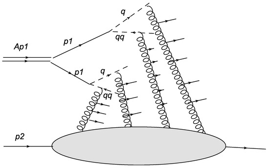
Figure 1.
collision for , with creation of four color strings; nucleons of the projectile are shown by solid lines, and the partons into which they split (quarks and diquarks) by dashed lines.
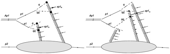
Figure 2.
collision for with creation of four color strings which fuse within individual nucleons (left panel) or between different nucleons (right panel). The nucleons of the projectile are shown by solid lines and the partons into which they split (quarks and diquarks) by dashed lines. Cumulative particles are shown by thick solid lines.
Let a parton from the projectile carry a part of the “+” component of nucleon momentum and let a partner parton from the target carry a part of the “−” component of nucleon momentum . The total energy squared for the colliding pair of nucleons is
where m is the nucleon mass and Y is the total rapidity. We assume that the energy is high, meaning that . The c.m. energy squared accumulated in the string is then
Note that the concept of a string only has sense in the case when s is not too small, say, more than . Thus, both and cannot be too small.
We relate the scaling variables for the string endpoints to their rapidities by
due to (4) and . The “length” of the string is simply the difference .
Due to partonic distribution in x, the strings have different lengths; moreover, they can take different positions in rapidity with respect to the center . The sea distribution in a hadron is much softer than the valence one. In fact, the sea distribution behaves as near , meaning that the average value of x for sea partons is small, on the order of [15]. As a result, strings attached to sea partons in the projectile nucleus carry very small parts of longitudinal momentum in the forward direction, and these fall with energy; as such, they seem to be useless for building up the cumulative particles. This allows us to retain only strings attached to valence partons, that is, quarks and diquarks, in the projectile while neglecting those strings attached to sea quarks altogether. This is reflected in Figure 1, where we show only the valence partons in the projectile. Note that the number of the former is exactly equal to , and does not change with energy. Thus, independent of the energy, for a given nucleus we always have a fixed number of strings.
The upper-end rapidities of the strings attached to diquarks are usually thought to be larger than those attached to the quarks, as the average value of x for the diquark is substantially larger than that for the quark. Theoretical considerations lead to the conclusion that, as , the distributions for the quark and diquark in the nucleon behave as and , respectively, modulo logarithms [15]. Neglecting the logarithms and taking into account the behavior at , we assume that these distributions for the quark and diquark are
and
The quark and diquark strings attach to all sorts of partons in the target nucleon, including valence quarks, diquarks, and sea quarks. However, their position in rapidity in the backward hemisphere is very different. Here, we are not interested in the spectrum in the backward hemisphere. For our purposes, limiting ourselves to the forward hemisphere, we may take the lower ends of the strings, which are all equal to . As a result, at the start of our model we have initially created strings, half of which are attached to quarks and half to diquarks, with their lower ends in rapidity all equal to
and their upper ends distributed in accordance with (5) and (6). As soon as they overlap in the transverse space, they fuse into new strings with more color and more energy. This process is studied in the next section.
3. Fragmentation Spectra and Fusion of Strings
3.1. One Sort of Strings and Particles
The following discussion closely follows that in [9]. To start, we study a simplified situation with only one type of string. We consider both the original string stretched between the partons of the projectile and target and the fused strings of higher color which are generated when n original strings occupy the same area in the transverse plane.
First, we consider the original simple string. Let it have its ends at and . For cumulative particles, we are interested only in the forward hemisphere and only in the “+” components of momenta; thus, in the following, we omit the subindex “+”.
We are interested in the spectrum of particles emitted from this string with longitudinal momentum . Evidently, x varies in the interval
or when introducing in the interval
The multiplicity density of produced particles (pions) is then
and the total multiplicity of particles emitted in one of the two hemispheres is
where is the total multiplicity in both hemispheres. The emitted particles have their “+” momenta in the interval
and, as ,
Thus, the particles emitted from the simple string cannot carry their “+” momenta greater than a single incoming nucleon. They are non-cumulative.
Now, let several simple strings coexist without fusion. Each of these strings produces particles in the interval dictated by its ends. If the ith string has its upper end , then the total multiplicity density of n unfused strings is
where is the multiplicity density of the ith string, and is different from zero in the interval
As a result, all produced particles have their “+” momenta lying in the same interval as that for a single string, meaning that they are all non-cumulative. We conclude that no cumulative particles will appear without string fusion. In this picture, only fusion of strings produces cumulative particles.
Now, consider that n simple strings fuse into a fused string. The process of fusion obeys two conservation laws, namely, those of color and momentum. As a result of the conservation of color, the color of a fused string is higher than that of an ordinary string [5,6]. Of the four momentum conservation laws, here we are mostly interested in the conservation of the “+” component, which leads to the conservation of x. A fused string has an upper endpoint
where are the upper ends of the fusing strings. This endpoint can be much higher than the individual of the fusing strings. In the limiting case when each fusing string has , we find . Consequently, the particles emitted from the fused string have maximal “+” momentum and are cumulative with the degree n of cumulativity.
At this point, we have to stress that there are several notable exceptions. The maximal value n for can be achieved only when different strings which fuse are truly independent, which is the case if the strings belong to different nucleons in the projectile. To picture this, imagine that two strings which belong to the same nucleon fuse, with one starting from the quark and the other from the antiquark. In this case, and have the same value as . Thus, fusing of strings inside the nucleon does not provide any cumulative particles. Such particles are only generated by fusing of strings belonging to different nucleons in the projectile; compare the left and right panels in Figure 2. In the left panel, the two fused strings come each from the same nucleon, and cannot generate cumulative particles; such configurations are to be dropped. In the right panel, the fused string is formed from strings belonging to different nucleons, resulting in cumulative paricles.
The multiplicity density of particles emitted from the fused string is denoted by
where is the generated multiplicity. It is different from zero in the interval
or again, introducing in the interval
We are interested in emission at high values of x, or of z close to unity, that is, in the fragmentation region for the projectile. Standardly, it is assumed that the multiplicity density is practically independent of x in the central region, that is, at small x. However, cannot be constant in the whole interval (7), and has to approach zero at its end in the fragmentation regions. At such values of z, is expected to strongly depend on z. Our task is to formulate the z-dependence of in this kinematical region.
To this end, we can set up certain sum rules which follow from the mentioned conservation laws and restrict possible forms of the spectrum of produced hadrons.
The total number of particles produced in the forward hemisphere by the fused string should be greater than by the ordinary string. This leads to the multiplicity sum rule:
where, as before, is the total multiplicity from a simple string in both hemispheres. The produced particles have to carry all the longitudinal momentum in the forward direction. This results in the following sum rule for x:
In these sum rules, is provided by (3) and is small. Passing to the scaled variable
we can rewrite the two sum rules as
and
where
These sum rules place severe restrictions on the form of the distribution , which obviously cannot be independent of n. Comparing (7) and (8), we can see that the spectrum of the fused string has to vanish at its upper threshold faster than is the case for the simple string. In the scaled variable z, it is shifted to smaller values, that is, to the central region. This must have a negative effect on the formation of cumulative particles produced at extreme values of x.
To proceed, we choose the simplest form for the distribution
with only two parameters: magnitude and slope .
The x sum rule relates and as follows:
The multiplicity sum rule finally determines via as
This equation can be easily solved when . We can present the integral in (14) as
The integral term is finite at ; thus, we can write it as a difference of integrals in the intervals and . The first can be found exactly:
The second term has an order and is small unless grows faster than n, which is not the case, as we shall presently see. In fact, we find that grows roughly as , which allows to neglect the second factor in (14) and rewrite it in its final form:
Note that the total multiplicity from a simple string is just Y; additionally, , meaning that
Thus, Equation (18) can be rewritten as
This transcendental equation determines for the fused string. Obviously, at the solution does not depend on and is just . To finally fix the distributions at finite Y, we have to choose the value of for the simple string. We take the simplest choice for an average string with , which corresponds to a completely flat spectrum and agrees with the results of [15]. This fixes the multiplicity density for the average string
which favorably compares to the value in 1.1 extracted from the experimental data [8]. After that, the equation for takes the form
At finite Y, this has to be solved numerically to provide , where is the upper end of the string n.
We find that with the growth of n the spectrum of produced particles goes to zero at more and more rapidly. Therefore, although strings with large n produce particles with large values of , the production rate is increasingly small.
3.2. Different Strings and Particles
In reality, strings are of two different types, attached to either quarks or antiquarks. Additionally, various types of hadrons are produced in general. In the cumulative region, the mostly studied particles are nucleons and pions, the production rates of the rest being much smaller. As mentioned in the introduction to this paper, the dominant mechanism for emission of cumulative nucleons is the spectator mechanism, which lies outside the color string picture. Thus, we restrict ourselves here to cumulative pions. The multiplicity densities for each sort of fused strings obviously depends on its flavor contents, that is, on the number of quark and diquark strings in it.
Let the string be composed of quarks and k diquarks, We then have distributions for the produced pions. The multiplicity and momentum sum rules alone are now insufficient to determine each of the distributions separately. To overcome this difficulty, we note that in our picture the observed pion is produced when the parton (quark or diquark) emerging from string decay neutralizes its color by picking up an appropriate parton from the vacuum. In this way, a quark may go into a pion if it picks up an antiquark or into a nucleon if it picks up two quarks. The rules for quark counting tell us that the behavior at the threshold in the second case has two extra powers of . Likewise, a diquark may either go into a nucleon by picking up a third quark or into two pions by picking up two antiquarks, with a probability smaller by a factor at the threshold. On the other hand, at the threshold the probability of finding a quark in the proton is smaller than that of the diquark; see Equations (5) and (6). These two effects, that of color neutralization and threshold damping in the nucleus, seem to compensate for each other, so that in the end the pion production rate from the antiquark string is only twice the rate of that from the quark string, provided the distribution of the former in the nucleus is the same as for the quark strings. This enables us to take the same distributions (5) for quark and antiquark strings in the nucleus, and to use
for the fragmentation function , where is the distribution (13) determined in the previous subsection. Equation (22) takes into account the doubling of pion production from antiquark strings. For the simple string, it correctly provides
Averaging (22) over all n-fold fused strings, we have the average ; thus, can be well approximated by
Note that should we wish to consider cumulative protons, then quark strings provide practically no contribution, being damped both at the moments of their formation and neutralized in terms of color. In contrast, antiquarks dominate at both steps, and provide effectively the total contribution. Thus, we would have to consider only antiquark strings and only one multiplicity distribution, that of nucleons , for which our sum rules are valid with the sole change , that being the total multiplicity of nucleons. However, it then becomes necessary to use distribution (6) for antiquark strings in the nucleus, which grows in the fragmentation region.
4. Nucleus–Nucleus Scattering
In the preceding sections, we studied scattering in the system where the nucleus is moving fast in the positive direction z. Correspondingly, we were interested in the forward hemisphere in the deep fragmentation region, with our attention focused on particles emitted with longitudinal momenta higher than that of the projectile nucleons. The role of the target proton was purely that of a spectator, as we were not interested in particles moving in the opposite direction from the projectile nucleus. The only information necessary about the target was that all strings attached to the projectile nucleus could be attached to the target. This was related to existence of sea partons in the target apart from the dominant valence ones.
If we instead substitute the nucleus (say, of the same atomic number A) for the proton target, nothing changes in the projectile nucleus hemisphere, and all our previous formulas remain valid. The only difference is that strings attached to the nucleons in the projectile nucleus can now be coupled to valence partons in the target nucleus, provided both nuclei overlap in the transverse area. Thus, the number of all strings depends on geometry, more concretely, on the impact parameter b. As for pA collisions, formation of cumulative strings with requires that the fusing strings belong to different nucleons in the projectile, meaning that the picture of cumulative production will not change except that in it will be different for different b. The final cumulative multiplicity is obtained as usual by integration over all values of the impact parameter b.
Thus, as far as the cumulative particles are concerned, the difference between and collisions reduces to the geometry in the transverse plane and the ensuing change in string configurations.
5. Probability of Cumulative Strings
5.1. Geometric Probability of String Fusion
As stressed previously, the cumulative production in our scenario is totally explained by the formation of fused strings, which follows when strings overlap in the transverse space. The exact nature of this overlapping may be different, i.e., total or partial. In the transverse space, such fused strings may have different forms and dimensions, presenting complicated geometrical structures. The detailed analysis of their geometry and dynamical properties presents an exceptionally complicated and hardly realizable task, even when the number of strings is quite small, to say nothing of the realistic case when this number is counted by hundreds or even thousands. However, the study of cases with a small number of strings shows that equivalent results can be well reproduced within a simplified picture [16]. To accomplish this, we can cover the transverse area of interaction by a lattice with cells having the areas of the simple strings (circles of radius fm). Strings stretched between the projectile and target appear in either one cell or in different cells. When a cell contains n strings, they are assumed to fuse and give rise to an n-fold fused string occupying this cell.
In this approach, the formation of fused strings proceeds in several steps. First, consider pA collisions. In the first step, the aforementioned lattice is set up to cover the whole area of the nucleus. Cells form the file , of their points in the transverse plane, with the center of the nucleus at .
The second step is to randomly add A nucleons at points with the probability provided by the transverse density . These are added successively, and with each new nucleon one passes to the third step.
The third step is to randomly add two strings around each of the added nuclei at distances from its center dictated by the appropriate matter density within the nucleon (Gaussian). Each of the two strings then arrives into some cell m which enhances its string content , by unity.
At this point, it is necessary to take into account that the types of two fusing strings, quark and antiquark, attached to the same nucleon in the projectile nucleus do not generate a cumulative string with their upper end (see Section 3.1). Thus, they must be excluded from the total set of fused strings, leaving only those which are generated when to the target two strings from different nucleons of the projectile nucleus are attached. To accomplish this, we first note that the two strings from the same nucleon may either be put in different cells and , or put in the same cell when . In the former case, both and are each enhanced by unity. In the latter case, does not change. As a result in the cumulative production a fused string is only generated when it belong to different nucleons in the projectile nucleus, meaning that they have to overlap in the transverse area. This introduces factor of smallness, which is roughly the ratio of the transverse areas of the nucleon to the nucleus for each successive fusion of strings; this is responsible for the fast decrease in the cumulative cross-section with the growth of cumulative number x.
In the fourth step, a search is performed for all cells with more than two strings, finding cells with two strings, that is, two-fold fused strings, cells with three strings, that is, three-fold fused strings, etc. Different cells mark the overlap of several nucleons at different locations in the transverse plane and physically mark different trajectories of the target proton at each collision. Thus, to find the total cross-section, we have to take the sum of contributions of all cells with a given number of strings n calculated with the relevant dynamical probability and particle distribution from Equation (13). This corresponds to the cross-section at all impact parameters b of the target proton as it crosses the nucleus.
Here, recall that the cumulative string with can only be formed when it starts from valence quarks in the projectile nucleus. Thus, only two strings can be attached to each nucleon, and the total number of simple strings is fixed to . On the contrary, for non-cumulative production the sea quarks in the projectile contribute to the number of strings from each nucleon, and the resulting multiplicity steadily increases with energy. From this, we can immediately conclude that cumulative production depends only very weakly on energy, with all of this dependence coming from powers .
For AA scattering, the procedure does not change, with the only difference being that the nuclei overlap is substituted for the projectile nucleus depending on the impact parameter b for the collision, resulting in different cumulative multiplicity for different b. The total multiplicity is obtained after integration over all b.
5.2. Probability of Cumulativity of a Fused String
Strings are distributed in the nucleons with probabilities (5) and (6) for quarks and diquarks. As argued above, we assume that they are all distributed with the quark distribution (5). To eliminate the steep growth at , we move to the variable . In terms of u, the distribution takes the simple form
The probability of finding a string with its upper end at x consisting of n simple strings with ends is provided by the multiple integral
We have to determine the limits of successive integrations starting from the -th. From the start, it is obvious that can be different from zero only in the interval .
For two strings, we have
Evidently, we should have
These two conditions determine the lower and upper limits and of integration over
or correspondingly the limits in
Probability is different from zero in the region of x such that .
- If , then and ; thus, .
- If , then and ; thus, , provided .
- If , then and ; thus, and , as noted previously.
In consequence, a nonzero result is obtained at , though with different integration limits. In the case of interest, that is, , the limits are and .
Now, consider for .
From (25), we find the recurrent relation
The limits
are determined by the condition , which limits to the region
From this, we find
For , it follows that is independent of x.
For a with respect to , we obtain . However, in the interval , we obtain .
Equation (29) can be used to calculate starting from , as explicitly provided by integral (26).
6. Calculations
For both proton–nucleus and nucleus–nucleus collisions, it is necessary to know the probabilities of fused string formation and the observed particle distribution . The former is determined by Equation (26) and the recurrent relation (29), while the latter is fully expressed by the powers , which in turn are determined by Equation (21) with . In fact, fused strings formed from more than five simple strings are not found in our calculations for either p-A or A-A collisions. For , the results of our numerical calculations provide and , which are presented in Figure 3, Figure 4 and Figure 5. At fixed , grows with n in accordance with Equation (21).
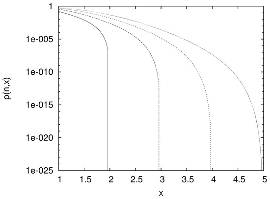
Figure 3.
Probabilities , which are different from zero in the interval .
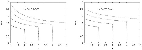
Figure 4.
Powers at 27.5 and 200 GeV. From bottom to top, the curves correspond to .
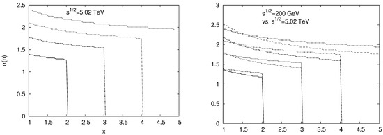
Figure 5.
Powers at TeV and comparison of GeV and TeV. From bottom to top, the curves correspond to . In the right panel, for each n the upper curve corresponds to the higher energy.
With these characteristics of cumulative string formation now known, we can begin the Monte Carlo procedure to finally find the string distributions and cumulative multiplicities. We performed 10,000 runs on our Monte Carlo program. For pA collisions, we chose p-Ta at 27.5 GeV. This case, involving comparatively low energies, is hardly suitable for our color string picture, as the length of cumulative strings is restricted by . However, we chose it having in mind the existing old experimental data on cumulative pion production [10,11]. For AA, we considered Cu–Cu and Au–Au collisions at 200 GeV (RHIC) and Pb–Pb collisions at 5.02 TeV (LHC).
6.1. p-Ta at 27.5 GeV
The described numerical calculation provides the numbers of fused strings (NFS) shown in Table 1 The data for provide the number of non-fused strings, and so on with . These data are provided only for the sake of comparing fused and non-fused strings. We would repeat here that these data refer only to the cumulative situation in which the number of strings is restricted to two for each nucleon in the nucleus; once leaving this restriction aside, these numbers will grow considerably and increase strongly with higher energy.

Table 1.
p-Ta at 27.5 GeV.
From these sets of strings, we can obtains the multiplicities per unit rapidity, which are shown in Figure 6.
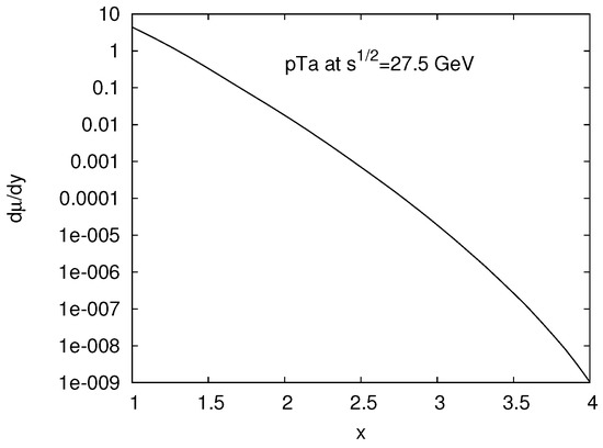
Figure 6.
Multiplicities per unit rapidity for production of cumulative pions at cumulativity in p-Ta collisions at 27.5 GeV.
6.2. AA
In this case, the distribution of cumulative strings and multiplicities depends on the impact parameter b. We split our results roughly into three categories depending on the value of b: central, with ; mid-central, with ; and peripheral, with , where fm is the effective “nucleus radius”. The distribution of cumulative strings is shown in Table 2, Table 3 and Table 4 for collisions Cu–Cu and Au–Au at 200 GeV and Pb–Pb at 5.02 TeV.
Table 2.
Cu–Cu at 200 GeV.
Table 3.
Au–Au at 200 GeV.
Table 4.
Pb–Pb at 5.02 TeV.
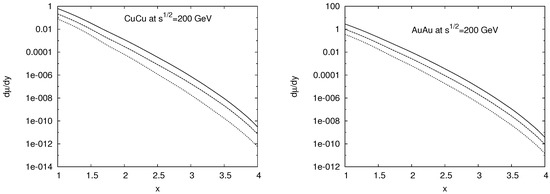
Figure 7.
Multiplicities per unit rapidity for production of cumulative pions at cumulativity in the central (upper curve), mid-central (middle curve), and peripheral (lower curve) regions in Cu–Cu and Au–Au collisions at 200 GeV.
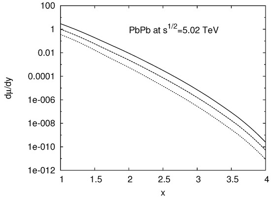
Figure 8.
Multiplicities per unit rapidity for production of cumulative pions at cumulativity in the central (upper curve), mid-central (middle curve), and peripheral (lower curve) regions in Pb–Pb collisions at 5.02 TeV.
The total multiplicities obtained after integration over all b are illustrated in Figure 9 and Figure 10.
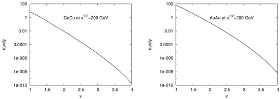
Figure 9.
Total multiplicities per unit rapidity for production of cumulative pions at cumulatively in Cu–Cu and Au–Au–Au collisions at 200 GeV.
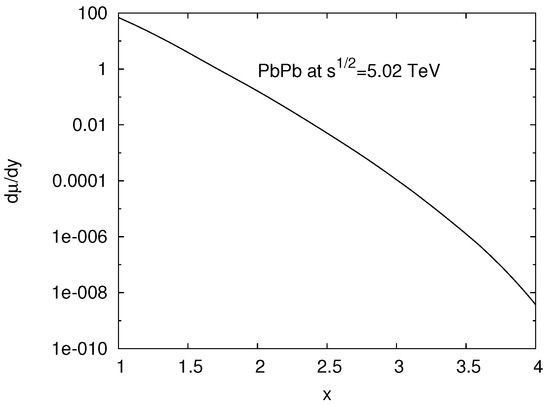
Figure 10.
Total multiplicities per unit rapidity for production of cumulative pions at cumulatively in Pb–Pb collisions at 5.02 TeV.
7. Discussion
In all cases, our obtained multiplicities as a function of cumulativity have a simple exponential form of :
The value of turns out to be of order five and varies weakly for different cases. For p-Ta at 27.5 GeV, we find . For Cu–Cu and Au–Au at 200 GeV, we obtain and 5.2, respectively. Finally, for Pb–Pb at 5.02 TeV we find . We do not see any conclusive explanation for this small variation, which may arise from the difference in energy, nuclear wave function, and insufficient number of runs. For the coefficient C, its value for p-Ta is 657 and for central Cu–Cu, Au–Au, and Pb–Pb its values are 166, 517, and 572, respectively.
Inspecting all cases, we see that cumulative production of pions shows a large degree of universality, which is typical for the fragmentation region of particle production. The slope of is to a very large degree explained by overlapping of individual nucleons in the nucleus, and is roughly derived from the probability of finding nucleons occupying the same area in the nucleus. It is essential, however, to note that overlapping of nucleons in the color string picture only occurs due to formation of strings, that is, interaction with the target. Thus, compared to the initial much older idea in the cumulative kinematics of the existence of “fluctons” in the nucleus with a larger mass and capable of producing particles, the string picture does not see fluctons in the nucleus from the start.
Very recent experimental study of cumulative production has been performed with Cu–Au collisions at 200 GeV [14]. Cumulative jets were detected with cm energy E greater than allowed by the proton–proton kinematics GeV. These data have been presented in two forms: raw data coming from the detectors, and so-called unfolded data, which presumably take into account distortions due to different sources in the concrete experimental setup. Remarkably, in the cumulative region the raw data fall exponentially as provided by (30), with a slope which does not practically depend on either centrality or jet characteristics. Our results in this paper refer instead to collisions of identical nuclei, such as Cu–Cu or Au–Au; however, as we have argued, the cumulative production in the projectile region does not depend on the target, the influence of which is only felt via the overlap in the transverse space. With different nuclei, the number of active nucleons will be different; nonetheless, in our picture this will influence only the magnitude of the production rate, not its x-dependence. Therefore, the observed slope agrees well with our predictions.
On the other hand, the unfolded data have a different x-dependence in the power form
with p and q adjusted to the data, and or 193 GeV depending on the cone width of the jet and not on the centrality. These unfolded data do not behave in accordance with our predictions. This discrepancy may proceed from our simplified picture of parton fragmentation (our partons go into pions with 100% probability), and certainly deserves better study both in terms of our treatment and in terms of any experimental subtleties.
As mentioned in our introduction, cumulative pions have been seen in the HIJING and DPMJET models of Cu–Au collisions. Because the authors of those studies were mostly interested in the overall spectra, no special attention and analysis were provided on the cumulative region. However, it is notable that they provided different predictions for cumulative pions (with more particles and greater energies in HIJING), and that in HIJING rather strong centrality dependence was found. This latter property contradicts both our model and experimental findings.
In conclusion, we would note that the flucton idea for cumulative production cannot be discarded altogether. It is possible to envisage formation of a very fast particle already taking place before the interaction. As mentioned in our introduction, cumulative production within this picture corresponds to the so-called spectator mechanism. It is to be expected that in this approach the leading particle will be one of the nucleons from the fast nucleus itself. The possibility of its formation was discussed in our older paper in the framework of a simple quark–parton model [4]. It was later shown that the spectator mechanism provides the bulk of the contribution for the cumulative protons, with the direct mechanism considered the earlier paper being suppressed [7]. This may explain why, when applied to cumulative proton production in p-Ta collisions at 27.5 GeV, the color string approach provides multiplicities two orders of magnitude smaller than those found by experiment [9].
Funding
This research received no external funding.
Conflicts of Interest
The author declares no conflict of interest.
References
- Baldin, A.M.; Giordenescu, N.; Ivanova, L.K.; Moroz, N.S.; Povtoreiko, A.A.; Radomanov, V.B.; Stavinsky, V.S.; Zubarev, V.N. An Experimental Investigation of Cumulative Meson Production. Sov. J. Nucl. Phys. 1975, 20, 629–634, Yad. Fiz. 1974 20 1201–1213. [Google Scholar]
- Strikman, M.I.; Frankfurt, L.L. High-energy phenomena, short-range nuclear structure and QCD. Phys. Rep. 1981, 76, 215–347. [Google Scholar]
- Efremov, A.V.; Kaidalov, A.B.; Kim, V.T.; Lykasov, G.I.; Slavin, N.V. Production of cumulative hadrons in quark models of flucton fragmentation. Sov. J. Nucl. Phys. 1988, 47, 868. [Google Scholar]
- Braun, M.A.; Vechernin, V.V. Nuclear structure functions and particle production in the cumulative region in the parton model. Nucl. Phys. B 1994, 427, 614. [Google Scholar] [CrossRef]
- Braun, M.A.; Pajares, C. Particle production in nuclear collisions and string interactions. Phys. Lett. B 1992, 287, 154. [Google Scholar] [CrossRef]
- Braun, M.A.; de Deus, J.D.; Hirsch, A.S.; Pajares, C.; Sharenberg, R.P.; Srivastava, B.K. De-confinement and clustering of color sources in nuclear collisions. Phys. Rep. 2015, 599, 1–50. [Google Scholar] [CrossRef]
- Braun, M.A.; Vechernin, V.V. Transverse-momentum dependence of cumulative pions. Phys. At. Nucl. 1997, 60, 506. [Google Scholar] [CrossRef]
- Braun, M.A.; Vechernin, V.V. On interference of cumulative proton production mechanisms. J. Phys. G Nucl. Part Phys. 1993, 19, 517. [Google Scholar] [CrossRef]
- Braun, M.F.; Ferreiro, E.G.; del Moral, F.; Pajares, C. Cumulative particle production and percolation of strings. Eur. Phys. J. C 2002, 25, 249. [Google Scholar] [CrossRef]
- Bayukov, Y.D.; Efremenko, V.I.; Frankel, S.; Frati, W.; Gazzaly, M.; Leksin, G.A.; Nikiforov, N.A.; Perdrisat, C.F.; Tchistilin, V.I.; Zaitsev, Y. Backward production of protons in nuclear reactions with 400 GeV protons. Phys. Rev. C 1979, 20, 764. [Google Scholar] [CrossRef]
- Nikiforov, N.A.; Bayukov, Y.; Efremenko, V.I.; Leksin, G.A.; Tchistilin, V.I.; Zaitsev, Y.; Frankel, S.; Frati, W.; Gazzaly, M.; Perdrisat, C.F. Backward production of pions and kaons in the interaction of 400 GeV protons with nuclei. Phys. Rev. C 1980, 22, 700. [Google Scholar] [CrossRef]
- Wang, X.N.; Gyulass, M. HIJING: A Monte Carlo model for multiple jet production in pp, pA, and AA collisions. Phys. Rev. D 1991, 44, 3501. [Google Scholar] [CrossRef] [PubMed]
- Engel, R. Photoproduction within the two-component Dual Parton Model: Amplitudes and cross sections. Z. Phys. C 1995, 66, 203–214. [Google Scholar] [CrossRef]
- Zhang, A.L.; Ridout, S.A.; Parts, C.; Sachdeva, A.; Bester, C.S.; Vollmayr-Lee, K.; Utter, B.C.; Brzinski, T.; Graves, A.L. Jammed solids with pins: Thresholds, force networks, and elasticity. Phys. Rev. C 2022, 106, 034902. [Google Scholar] [CrossRef] [PubMed]
- Capella, A.; Sukhatme, U.P.; Tan, C.-I.; Tran Thanh Van, J. Dual parton model. Phys. Rep. 1994, 236, 225–329. [Google Scholar] [CrossRef]
- Braun, M.A.; Kolevatov, R.S.; Pajares, C.; Vechernin, V.V. Correlations between multiplicities and average transverse momentum in the percolating color strings approach. Eur. Phys. J. C 2004, 32, 535–546. [Google Scholar] [CrossRef]


Disclaimer/Publisher’s Note: The statements, opinions and data contained in all publications are solely those of the individual author(s) and contributor(s) and not of MDPI and/or the editor(s). MDPI and/or the editor(s) disclaim responsibility for any injury to people or property resulting from any ideas, methods, instructions or products referred to in the content. |
© 2023 by the author. Licensee MDPI, Basel, Switzerland. This article is an open access article distributed under the terms and conditions of the Creative Commons Attribution (CC BY) license (https://creativecommons.org/licenses/by/4.0/).