Article

Scalar Product for a Version of Minisuperspace Model with Grassmann Variables

by
Sergey L. Cherkas
1,*,† and
Vladimir L. Kalashnikov
2,†
1
Institute for Nuclear Problems, Bobruiskaya 11, 220006 Minsk, Belarus
2
Department of Physics, Norwegian University of Science and Technology, 7491 Trondheim, Norway
*
Author to whom correspondence should be addressed.
These authors contributed equally to this work.
Universe 2023, 9(12), 508; https://doi.org/10.3390/universe9120508
Submission received: 17 April 2023 / Revised: 4 November 2023 / Accepted: 28 November 2023 / Published: 7 December 2023
(This article belongs to the Special Issue Recent Advances in Quantum Cosmology)

Abstract

:
Grassmann variables are used to formally transform a system with constraints into an unconstrained system. As a result, the Schrödinger equation arises instead of the Wheeler–DeWitt one. The Schrödinger equation describes a system’s evolution, but a definition of the scalar product is needed to calculate the mean values of the operators. We suggest an explicit formula for the scalar product related to the Klein–Gordon scalar product. The calculation of the mean values is compared with an etalon method in which a redundant degree of freedom is excluded. Nevertheless, we note that a complete correspondence with the etalon picture is not found. Apparently, the picture with Grassmann variables requires a further understanding of the underlying Hilbert space.

1. Introduction

There is a principal possibility to construct the theory of quantum gravity (QG) from the point of view that gravity is a usual physical system with constraints [1,2]. As a result, it has to be quantized using Dirac brackets [3].
The physical question arises: what type of gravity theory must be quantized? It is hardly general relativity (GR), because GR suffers from the loss of information (unitarity) in black holes [4,5] (however, see, e.g., [6,7,8]) and from the vacuum energy problem [9,10,11]. It seems possible [12] to repair GR by restricting it to a class of submanifolds without black holes [13,14]. Simultaneously, the possibility of arbitrarily choosing an energy density level appears [12,15], which removes the vacuum energy problem, at least for massless particles. Contributions of the masses of particles into vacuum energy density M p 2 m 2 have to be mutually compensated for [16]. Contributions of the order of m 4 also have to be compensated for but by taking condensates into account [15]. The resulting theory, which has features such as partial gauge fixing, preferred reference frame, and the existence of æther [17,18] (in the form of condensates and vacuum polarization) could be a suitable candidate for quantization.
Another (mathematical) question is how to realize the commutation relations corresponding to Dirac brackets, which again implies gauge fixing by defining auxiliary conditions to convert a system from the first class to the second class. So far, there is no constructive way to do so generally [19]. In particular, the implementation of Dirac brackets in 3 + 1 GR has not yet been achieved. Even for 2 + 1 gravity, Dirac brackets have a rather complicated structure [20]. Moreover, in the case of gravity quantization, the gauge-fixing conditions must be time-dependent to introduce time into the theory. Instead, one could use the quasi-Heisenberg picture [21,22,23,24], where the commutator relations corresponding to Dirac brackets are determined at some fixed moment of time, e.g., near a small-scale factor that simplifies a problem.
A more radical method is introducing Grassmann variables [25,26,27,28,29,30], which formally reduces a system with constraints to an unconstrained one. However, if one applies Grassmann variables to calculate not only the scattering amplitudes but also the mean values of operators, the questions about Hilbert spaces and scalar products arise [31,32,33].
For simplicity, the question about scalar products could be considered in a minisuperspace model example. Minisuperspace models represent examples of simple systems with constraints and are widely used [34,35,36,37,38,39,40,41,42,43] to understand the main features of gravity quantization. Without experimental data for the minisuperspace model, one would not be able to straightforwardly check different approaches to gravity quantization. Fortunately, an etalon quantization method for the minisuperspace model that “could not be wrong” exists. It consists of the explicit exclusion of the redundant degree of freedom, initially, to obtain a physical Hamiltonian [44,45] through explicit gauge fixing. Considering this “etalon” method implies that QG has to violate gauge invariance. Certainly, opposite points of view exist; e.g., loop quantum gravity promises “covariant with respect to diffeomorphisms” QG [46] (however, see some comments in [47]).

2. The Etalon Picture with the Exclusion of the Redundant Degrees of Freedom

Let us consider the action functional of gravity minimally coupled to a massless scalar field:
S = 1 16 π G R g d 4 x + 1 2 𝜕 μ ϕ g μ ν 𝜕 ν ϕ g d 4 x ,
where R is the scalar curvature; Greek indexes run from 0 to 3; G is the Newton constant; g μ ν is the metric tensor, with g being its determinant. Considering a uniform, isotropic, and flat universe
d s 2 = g μ ν d x μ d x ν = a 2 ( N 2 d η 2 d 2 r ) ,
where functions a and N depend only on η , reduces action (1) to
S = 1 2 1 N M p 2 a 2 + a 2 ϕ 2 d η = p a a + π ϕ ϕ N 1 2 p a 2 + π ϕ 2 2 a 2 d η ,
where the reduced Planck mass, M p = 3 4 π G , is used, which is set to unity everywhere further for simplicity. The Hamiltonian
H = N 1 2 p a 2 + π ϕ 2 2 a 2 ,
also determines the Hamiltonian constraint
Φ 1 = 1 2 p a 2 + π ϕ 2 2 a 2 = 0 ,
by virtue of δ S δ N = 0 . The time evolution of an arbitrary observable A is expressed with the Poisson brackets
d A d η = 𝜕 A 𝜕 η + { H , A } ,
which are defined as
{ A , B } = 𝜕 A 𝜕 π ϕ 𝜕 B 𝜕 ϕ 𝜕 A 𝜕 ϕ 𝜕 B 𝜕 π ϕ 𝜕 A 𝜕 p a 𝜕 B 𝜕 a + 𝜕 A 𝜕 a 𝜕 B 𝜕 p a .
The full system of equations of motion has the form
ϕ = 𝜕 H 𝜕 π ϕ = N π ϕ a 2 , π ϕ = 𝜕 H 𝜕 ϕ = 0 , π ϕ = k = c o n s t ,
a = 𝜕 H 𝜕 p a = N p a , p a = 𝜕 H 𝜕 a = N k 2 a 3 .
The additional time-dependent gauge-fixing condition
Φ 2 = a 2 | π ϕ | η
can be introduced as the constraint Φ 2 , which fixes N to be equal unity. The condition (10) also fixes the direction of time because the scale factor increases with time. The solutions of Equation (9) are
a = 2 | π ϕ | η , ϕ = π ϕ 2 | π ϕ | ln η + c o n s t .
The constraints Φ 1 , Φ 2 allow reducing this simple system to a sole degree of freedom. Let us make some general notes about the exclusion of the variables and coming to the physical Hamiltonian. Let system variables be Q 1 , , Q m , q m + 1 , , q n , P 1 , , P m , p m + 1 , , p n and one would like to exclude n m coordinates q k and momentums p k using the constraints and additional conditions Φ k , to have only the variables Q k and momentums P k finally. Equating the Lagrangians before and after exclusion leads to
k = 1 m P k d Q k + k = m + 1 n p k d q k k = m + 1 m λ k Φ k = k = 1 m P k d Q k H p h y s ( Q , P ) d τ + d F ( Q , P , τ ) ,
where the left-hand part of (12) contains all the constraints, including the Hamiltonian one, whereas the right-hand side contains the full differential of some function F ( Q , P , τ ) . At the constraint surface Φ k , Equation (12) reduces to
H p h y s = k = m + 1 n p k q k + d F ( Q , P , τ ) d τ .
The function F has to be chosen in such a way that H p h y s reproduces correct equations of motion by
Q = 𝜕 H p h y s 𝜕 P , P = 𝜕 H p h y s 𝜕 Q .
Let us take π ϕ and ϕ as physical variables, then a and p a have to be excluded by the constraints. Substituting p a , a and a into (3) results in
L = π ϕ ϕ H p h y s ( ϕ , π ϕ , η ) d η ,
where
H p h y s ( ϕ , π ϕ , η ) = p a a = | π ϕ | 2 η .
Hamiltonian (16) reproduces the equations of motion (8) correctly; thus, function F in (13) equals zero for this particular case1.
The most simple and straightforward way to describe quantum evolution is to formulate the Schrödinger equation
i 𝜕 η Ψ = H ^ p h y s Ψ
with the physical Hamiltonian (16). In the momentum representation, the operators become
π ^ ϕ = k , ϕ ^ = i 𝜕 𝜕 k .
The solution of Equation (17) is written as
Ψ ( k , η ) = C ( k ) 2 e | k | η i | k | / 2 .
It is possible to calculate the mean values of an arbitrary operator A ^ ( k , i 𝜕 𝜕 k ) built from ϕ ^ = i 𝜕 𝜕 k and a = 2 | k | η with respect to a wave packet C ( k ) in the following way
< C | A ^ | C > = Ψ ( k , η ) A ^ Ψ ( k , η ) d k .
Since the basic wave function 2 e | k | η i | k | / 2 contains a module of k, a singularity may arise at k = 0 if A ^ contains degrees of the differential operator 𝜕 𝜕 k . That may violate hermicity. To avoid this, the wave packet has to be turned to zero at k = 0 . For instance, it could be taken in the Gaussian form
C ( k ) = 2 σ 5 / 2 3 π 1 / 4 k 2 exp ( k 2 / ( 2 σ 2 ) )
with the multiplier k 2 in the front of the exponent.
Let us come to the calculation of some mean values taking the parameter σ = 1 . The mean value of a 2 is2
< C | a 2 | C > = 16 3 π η 0 e k 2 k 5 d k = 16 3 π η .
The next quantity is expressed as
< C | a 4 | C > = 16 3 π η 2 e k 2 k 6 d k = 10 η 2 .
Other mean values for this wave packet were calculated in [45].

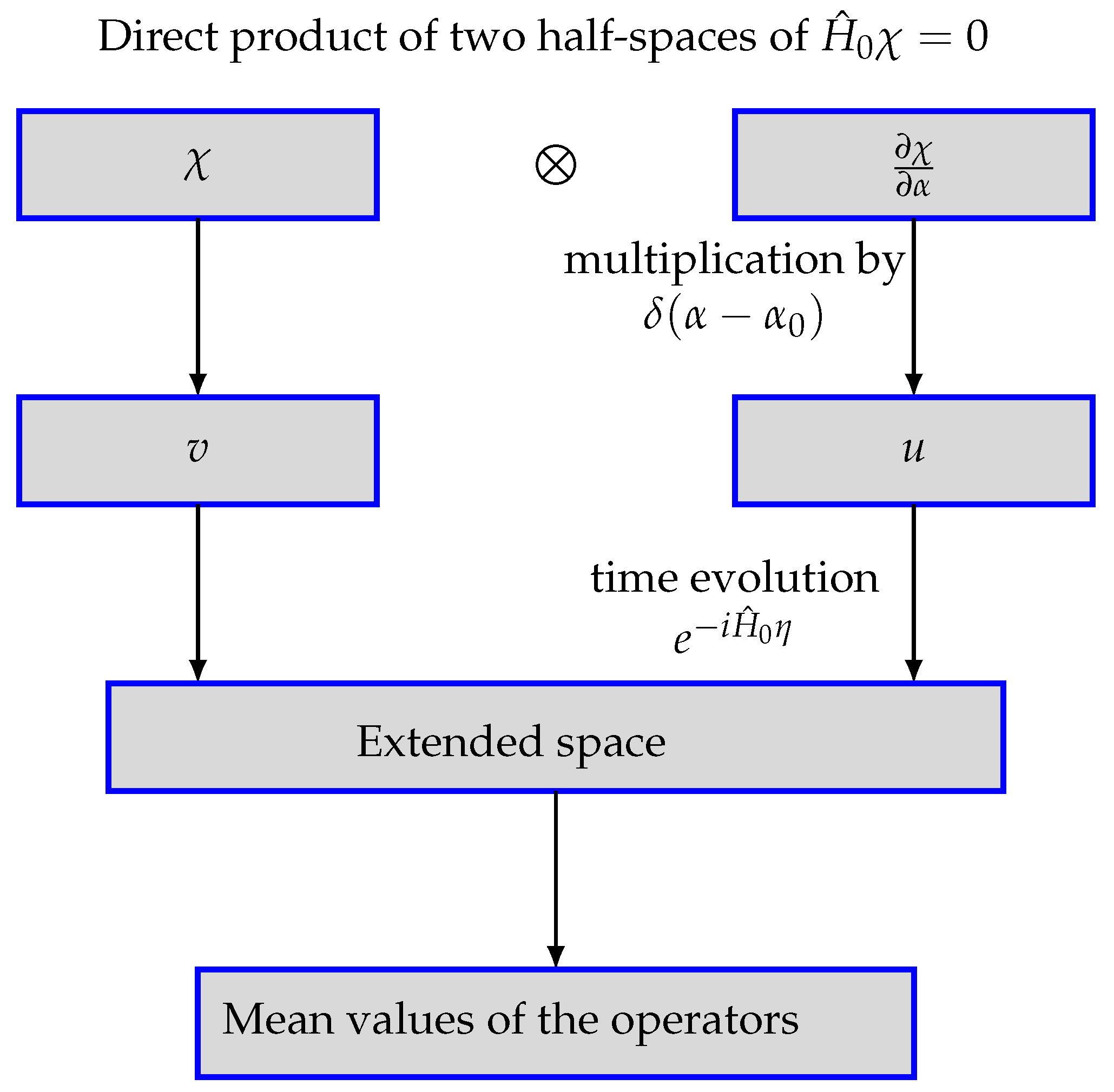
3. Evolution in Extended Space

Another derivation of the physical Hamiltonian (16) is given by the continual integrals considering the transition amplitude from in to out states. Using canonical gauge fixing condition Φ 2 = a 2 η | π ϕ | leads to
< o u t | i n > = Z = e i π ϕ ϕ p a a N 1 2 p a 2 + π ϕ 2 2 a 2 d η Π η Δ F P Π η δ Φ 2 D N D p a D a D π ϕ D ϕ = e i π ϕ ϕ p a a d η Π η p a Π η δ 1 2 p a 2 + π ϕ 2 2 a 2 Π η δ a 2 η | π ϕ | D p a D a D π ϕ D ϕ = e i π ϕ ϕ | π ϕ | / ( 2 η ) d η D π ϕ D ϕ .
Under the derivation of (24), it was used that Δ F P = { Φ 1 , Φ 2 } = p a , and Π η δ 1 2 p a 2 + π ϕ 2 2 a 2 = Π η δ p a | π ϕ | / a Π η p a . From (24) follows the formula (16) for a physical Hamiltonian. A principle of derivation is clear: obtaining an expression of a kind e i i p i q i H ( p , q ) d η D p D q without any pre-exponential factors and extracting H ( p , q ) to use in the Schrödinger equation.
However, the etalon picture with H p h y s cannot be applied in the general case to QG because one cannot resolve the constraints. It is believed that the Grassmann variables allow writing the Lagrangian in a form where there are no constraints [27,28,50,51,52]. Using non-canonical gauge fixing [31,53] leads to
Z = e i π ϕ ϕ p a a N 1 2 p a 2 + π ϕ 2 2 a 2 d η Π η δ F δ ε Π η δ ( F ) D p a D a D π ϕ D ϕ D N ,
where F ( N ) is a gauge-fixing function.
The action (3) is invariant under the infinitesimal gauge transformation:
a ˜ = a + δ a = a + ε a ,
ϕ ˜ = ϕ + δ ϕ = ϕ + ε ϕ ,
N ˜ = N + δ N = N + ( N ε ) ,
where ε is an infinitesimal function of time. If one takes the differential gauge condition F = N = 0 , then (28) follows in
δ F = δ N = ( N ε ) ,
and the Faddev–Popov determinant [53] takes the form of Δ F P = δ F δ ε = δ N δ ε = N + 2 N 𝜕 𝜕 η + N 𝜕 2 𝜕 η 2 . The functional (25) could be rewritten as
Z = e i π ϕ ϕ p a a N 1 2 p a 2 + π ϕ 2 2 a 2 θ ¯ ( N θ ) d η Π η δ ( N ( η ) ) D N D p a D a D π ϕ D ϕ D θ D θ ¯ = e i π ϕ ϕ p a a N 0 1 2 p a 2 + π ϕ 2 2 a 2 θ ¯ θ d η D p a D a D π ϕ D ϕ D θ D θ ¯ = e i π ϕ ϕ p a a + θ ¯ π θ ¯ + π θ θ N 0 1 2 p a 2 + π ϕ 2 2 a 2 + π θ π θ ¯ d η D p a D a D π ϕ D ϕ D π θ D π θ ¯ D θ D θ ¯ ,
where using the Grassmann variables [53] in the first equality of (30) raises the Faddeev–Popov determinant into an exponent. Here, a Grassmann number θ ¯ is considered as a complex conjugate to θ . Integration over N has been performed explicitly in (30). If N ( η ) is discretized over the interval Δ η , the term containing a product of the delta functions Π η δ ( N ( η ) ) takes the form
δ N 0 N 1 Δ η δ N 1 N 2 Δ η δ N k 1 N k Δ η d N 1 d N k 1 Δ η k 1 δ ( N 0 N k ) ,
i.e., an initial value of N 0 has to equal a final value N k , for instance, one may take N 0 = 1 . For deducing third equality of (30), see Appendix A. Extracting the Lagrangian from (30) gives
L = π ϕ ϕ p a a + θ ¯ π θ ¯ + π θ θ 1 2 p a 2 + π ϕ 2 2 a 2 + π θ π θ ¯ .
The action (32) is a fixed gauge action with no Hamiltonian constraint, but instead, the ghost (Grassmann) variables arise in (32).
Following Vereshkov and Shestakova et al. [27,28], one may consider the Hamiltonian
H = 1 2 p a 2 + π ϕ 2 2 a 2 + π θ π θ ¯
as describing the quantum evolution of a system.
To quantize the system, the anticommutation relation has to be introduced for the Grassmann variables
{ π θ , θ } = i , { π θ ¯ , θ ¯ } = i .
In the particular representation α = ln a , p ^ α = i 𝜕 𝜕 α , ϕ ^ = i 𝜕 𝜕 k , π ^ ϕ = k , π ^ θ = i 𝜕 𝜕 θ , π ^ θ ¯ = i 𝜕 𝜕 θ ¯ , the Schrödinger equation reads as
i 𝜕 𝜕 η ψ = 1 2 e 2 α 𝜕 2 𝜕 α 2 + k 2 𝜕 𝜕 θ 𝜕 𝜕 θ ¯ ψ ,
where the operator ordering in the form of the two-dimensional Laplacian [54] has been used3. It should be supplemented by the scalar product
< ψ 1 | ψ 2 > = ψ 1 ( η , k , α , θ ¯ , θ ) ψ 2 ( η , k , α , θ ¯ , θ ) e 2 α d α d k d θ d θ ¯ ,
where the measure e 2 α arises due to the hermicity requirement [26,54]. This measure is a consequence of a minisuperspace metric if the classical Hamiltonian is written in the form of H = 1 2 G i j p i p j + π θ π θ ¯ with p i { p α , π ϕ } , G i j = d i a g { e 2 α , e 2 α } . Thus, the measure takes the form G = e 2 α , G = | det G i j | and the Laplacian 1 G 𝜕 𝜕 q i G G i j 𝜕 𝜕 q i = e 2 α 𝜕 2 𝜕 α 2 + π ϕ 2 is self-adjoined [54] with this measure. Formal solutions of the Equation (35) can be written as
ψ ( η , k , α , θ ¯ , θ ) = ( θ ¯ + θ ) u ( η , k , α ) + i ( θ ¯ θ ) v ( η , k , α ) ,
where the functions u and v satisfy the equation
i 𝜕 𝜕 η u = H ^ 0 u
with
H ^ 0 = 1 2 e 2 α 𝜕 2 𝜕 α 2 + k 2 .
Then, the scalar product (36) reduces to
< ψ 1 | ψ 2 > = 2 i u 1 v 2 v 1 u 2 e 2 α d α d k .
Although the constraint H 0 = 0 formally disappears from the theory, one may think that the space of solutions of the Wheeler–DeWitt equation (WDW) still plays a role [33]. Otherwise, the question of correspondence with the classical theory, where the Hamiltonian constraint holds, arises. We would like to relate the space of the functions, satisfying the Schrödinger Equation (35) with the functions χ satisfying the equation H 0 χ = 0 , i.e., the WDW equation. The operator H ^ 0 (39) has the Klein–Gordon form. Thus, the Klien–Gordon-type scalar product has to be used. According to this hypothesis, let us represent the functions u, v as
  v ( α , k ) = e i H 0 η D ^ 1 / 4 χ ( α , k ) ,
u ( α , k , η ) = e i H 0 η D ^ 1 / 4 δ ( α α 0 ) 𝜕 𝜕 α χ ( α , k ) ,
where the operator D ^ = 𝜕 2 𝜕 ϕ 2 , or D = k 2 in the representation (18) and
χ ( α , k ) = e i α | k | α 0 2 | k | C ( k ) ,
and, as in (19), only a half-space corresponding to the negative frequencies’ solutions of the WDW equation is taken because only in this case does the Klein–Gordon product imply a positive definite norm of a state. The operator D ^ (see Appendix in [57]) is a necessary attribute of the scalar product for the Klein–Gordon equation to obtain hermicity. It should be noted that in fact, the function v does not depend on the time η because H ^ 0 χ = 0 and D ^ commutes with H 0 . Thus, the time evolution arises only due to function u, or more accurately, due to the presence of the Dirac delta function in (42).
Thus, the scalar product (40) reduces to
< ψ 1 | ψ 2 > = 2 i 𝜕 χ 1 𝜕 α χ 2 χ 1 𝜕 χ 2 𝜕 α e 2 α | α = α 0 d k .
The expression for the mean value of an operator A ^ has the form:
< ψ | A ^ | ψ > = 2 i e 2 α u A ^ v v A ^ u | α = α 0 d k ,
where u, v are given by (41) and (42), and it is assumed that an operator A ^ does not contain the ghost variables θ , θ ¯ , that is expected for physical operators. The limit α in (45) implies that an evolution begins at η = 0 when a = 0 and α = ln a tends to .
The evaluation of the mean values is illustrated schematically in Figure 1. Initially, we start with the negative frequency functions χ , 𝜕 χ 𝜕 α both satisfying H 0 χ = 0 . A direct product of these half-spaces is taken. Then, the function 𝜕 χ 𝜕 α is multiplied by δ ( α α 0 ) and runs into an extended space, where “evolution” occurs, and, thus, the mean values of the operators can be evaluated.
Both Schrödinger and Heisenberg pictures are possible with this scalar product. In the Heisenberg picture, the time-dependent operators have the form
A ^ ( η ) = e i H ^ 0 η A ^ e i H ^ 0 η ,
while the functions u and v have to be used without multiplier e i H ^ 0 η .

4. Expectation Values of Scale Factor Degrees

The simplest way to test a theory is to compare it with the etalon picture by calculating the mean value of the squared scale factor, which has to be equal to 16 3 π η according to (22). To do that, it is sufficient to expand e i H ^ 0 η 1 i H ^ 0 η 1 2 H ^ 0 2 η 2 in (41) and (42) and perform the calculation according (45). It turns out that the mean value of a 2 = e 2 α actually coincides with that given by (22). The next test is the calculation of < C | a 4 | C > . The result of the calculation is
< C | a 4 | C > = 2 η 2 ,
while the etalon model gives another value (23). The origin of this discrepancy could be better seen in the Heisenberg picture. Evolution equations for the Heisenberg operators follow from the operator commutators with the Hamiltonian (39)
d a ^ 2 d η = i [ H ^ 0 , a ^ 2 ] .
It is possible to guess a solution for this particular case:
a ^ 2 ( η ) = e 2 α + 2 η e α p ^ α e α 2 η 2 H ^ 0 ,
where we define p ^ α = i 𝜕 𝜕 α 4.
Actually, the calculation of the commutator (48) using (39), (49) gives
i [ H ^ 0 , a ^ 2 ( η ) ] = 2 e α p ^ α e α 4 η H ^ 0 ,
which is exactly equal to the derivative of (49) over η . Under calculation of the mean value of < C | a ^ 2 | C > , the third term in (49) does not contribute, and the result coincides with that of the etalon method. However, under the calculation of < C | a ^ 4 | C > , the first and third terms in (49) play a role, and the discrepancy with the etalon method arises. One can calculate the mean values of the other degrees of a, which are presented in Table 1. It is interesting to plot the values of k 2 n n = 1 η < C | a ^ 2 n ( η ) | C > n , which is shown in Figure 2.
Recently, analog models of QG and minisuperspace have been discussed [58,59]. In Appendix B, quantization of a particle-clock is considered, which has some similar features to the minisuperspace model but does not have an operator ordering issue.

5. Discussion and Conclusions

A reasonable expression for the scalar product using the Grassmann variables is suggested. It establishes a relation of a picture with the Grassmann variables to the Klein–Gordon scalar product and allows calculating the mean values of operators in both Schrödinger and Heisenberg pictures, which give the same results. However, it is shown that the mean values of a 2 n are different for n > 1 than those calculated in the etalon method, implying an explicit exclusion of the superfluous degrees of freedom. One may guess that the above methods could have different Hilbert spaces. That means that the different wave packets have to be taken for these methods to obtain the same set of operator mean values. Here, we cannot find a wave packet C ˜ ( k ) , which would give the same mean values as a wave packet C ( k ) for the etalon method.
The possible influence of the Zitterbewegung phenomenon in extended space was investigated in Appendix C but without a breakthrough in the results achieved. It should be noted that the quasi-Heisenberg picture corresponds entirely with the etalon method [45].
One of the possible ways to correct the picture with the Grassmann variables is to assume that the operators of physical observables act not only in k and α space but also in the extended space of the Grassmann variables θ , θ ¯ . This hypothesis needs further investigation5 as well as the general issue of the scalar product for the approach with the Grassmann variables.

Author Contributions

Concepts and methodology are developed by S.L.C. and V.L.K.; software, S.L.C.; validation, writing and editing, S.L.C. and V.L.K. All authors have read and agreed to the published version of the manuscript.

Funding

This research received no external funding.

Data Availability Statement

Data are contained within the article.

Conflicts of Interest

The authors declare no conflict of interest.

Appendix A. Generalized Hamiltonian Form of the Action with the Grassmann Variables

Let us prove the equivalence of the action functional with the Grassmann variables in the generalized Hamiltonian form to the conventional action in the Lagrangian form. Stating from Z θ in the generalized Hamiltonian form, let us use the invariance of the continual integral relative change of the variables [53]. Implementing the change π θ = ξ + θ ¯ and π θ ¯ = ξ ¯ + θ , we have
Z θ = e i θ ¯ π θ ¯ + π θ θ π θ π θ ¯ d η D π θ D π θ ¯ D θ D θ ¯ = e i θ ¯ ( ξ ¯ + θ ) + ( ξ + θ ¯ ) θ ( ξ + θ ¯ ) ( ξ ¯ + θ ) d η D ξ D ξ ¯ D θ D θ ¯ = e i ξ ¯ ξ d η D ξ D ξ ¯ e i θ ¯ θ d η D θ D θ ¯ e i θ ¯ θ d η D θ D θ ¯ ,
where a multiplier containing the integral over ξ , ξ ¯ is omitted in the last equality.
Certainly, another way to prove the equivalence is to find the momentums by varying the action
S θ = θ ¯ π θ ¯ + π θ θ π θ π θ ¯ d η
over π θ , π θ ¯ . That gives
π θ = θ ¯ , π θ ¯ = θ .
Then, substitution of the momentums (A3) into (A2) results in
S θ = θ ¯ θ d η .

Appendix B. Quantization of a Particle-Clock

It is interesting to consider the scalar product introduced above by giving an example of a relativistic particle, having its own clock (see Figure A1). It could be a radioactive particle decaying exponentially with a probability
P ( τ ) = 1 T e τ / T ,
where T is a mean lifetime of the particle. We will consider τ as a proper time of a system.
Figure A1. (a) Observer describing a particle motion by his clock, (b) description of a particle motion by “particle clock”.
Universe 09 00508 g0a1
The action of a relativistic particle can be defined as [53]:
S = 1 2 ( e 1 x ˙ μ 2 e m 2 ) d τ ,
where the x μ = { t , x } , ( , + , + , + ) signature is used, and the lapse function e ( τ ) is introduced. One more equivalent form resulting in (A6) after varying over p μ looks as
S = p μ x ˙ μ e p μ 2 + m 2 2 d τ = p x p t t e 2 p t 2 + p 2 + m 2 d τ .
From (A7), it follows that the particle analog of the minisuperspace Hamiltonian (4) is written as
H = e 2 ( p t 2 + p 2 + m 2 ) ,
and it is constraint Φ 1 simultaneously. The equations of motion are
d x d τ = 𝜕 H 𝜕 p = e p , p = c o n s t , d t d τ = 𝜕 H 𝜕 p t = e p t , p t = c o n s t .
The additional, depending on τ , gauge-fixing condition
Φ 2 = t p 2 + m 2 m τ = 0 ,
assigns e = 1 / m and after calculations (13), (14) leads to the physical Hamiltonian
H p h y s = p t t + d F ( p , τ ) d τ = p 2 + m 2 m + 𝜕 F ( p , τ ) 𝜕 τ
describing a particle motion in the proper time τ . In Equation (A11), the total derivative is changed by the partial derivative because momentum p does not depend on time. On the other hand, the physical Hamiltonian must reproduce motion in the reduced space to give
x = 𝜕 H p h y s 𝜕 p = p m ,
thus, 𝜕 F ( p , τ ) 𝜕 τ = p 2 + m 2 2 m and
H p h y s = p 2 + m 2 2 m .
Analogously to (17)–(20), a quantum picture with the Grassmann variables leads to the Schrödinger equation
i 𝜕 𝜕 η ψ = 1 2 m 𝜕 2 𝜕 t 2 + p 2 + m 2 𝜕 𝜕 θ 𝜕 𝜕 θ ¯ ψ .
The mean value of the operator A ^ ( t , i 𝜕 𝜕 t , p , i 𝜕 𝜕 p ) has the form:
< ψ | A ^ | ψ > = 2 i u A ^ v v A ^ u | t = t 0 0 d 3 p ,
where u, v are given by
v ( t , p ) = D 1 / 4 χ ( t , p ) ,
u ( t , p , τ ) = e i H 0 τ D 1 / 4 δ ( t t 0 ) 𝜕 𝜕 t χ ( t , p ) ,
H 0 = 1 2 m 𝜕 2 𝜕 t 2 + p 2 + m 2 ,
D = ε 2 ( p ) = m 2 + p 2 , and
χ ( t , p ) = e i ε t 2 ε C ( p ) .
For the wave packet
C ( p ) e ( p p 0 ) 2 / ( 2 σ 2 ) ,
the mean value of < ψ | t 2 | ψ > equals
< ψ | t 2 | ψ > = τ 2 ε 0 2 + 3 σ 2 m 2 ,
where ε 0 2 = p 0 2 + m 2 . It turns out to be the same for both methods: the physical Hamiltonian and that with the Grassmann variables. Calculation of the mean value of < ψ | t 4 | ψ > gives
< ψ | t 4 | ψ > = τ 4 ε 0 4 + 2 σ 2 5 ε 0 2 2 m 2 + 15 σ 4 m 4
for the physical Hamiltonian method and
< ψ | t 4 | ψ > = τ 4 ε 0 4 + 2 σ 2 5 ε 0 2 2 m 2 + 15 σ 4 m 4 3 τ 2 m 2
for the method with the Grassmann variables. Compared to Equation (A22), the additional term 3 τ 2 m 2 appears in (A23). The value of (A23) averaged over probability of particle decay (A5) leads to a quantity, which could be, in principle, observed experimentally:
0 < ψ | t 4 | ψ > P ( τ ) d τ = 24 T 4 ε 0 4 + 2 σ 2 5 ε 0 2 2 m 2 + 15 σ 4 m 4 6 T 2 m 2 .
The last term in (A24) becomes considerable when the particle width Γ = 1 / T is comparable with the particle mass.

Appendix C. Removing of an “Extended Zitterbewegung”

The well-known phenomenon of Zitterbewegung (see [61,62] and references therein) is an inevitable feature of any relativistic field equation and is usually removed by the Foldy–Wouthuysen transformation [63,64,65]. It arises due to interference of the solutions of the Klein–Gordon equation with the positive and negative frequencies. Here, we discuss the solution of the Schrödinger Equation (38) with the WDW operator on the right-hand side and will consider a possible “extended Zitterbewegung”. In the extended space, the solutions of the Schrödinger Equation (38) look as u λ = e i λ η ψ λ where the eigenfunctions ψ λ satisfy
H 0 ψ = λ ψ λ
with a different sign of λ . For λ > 0 , the general solution takes the form
ψ λ = c 1 J i | k | ( 2 λ e α ) + c 2 J i | k | ( 2 λ e α ) ,
where J i | k | is the Bessel function of an imaginary index. The solutions for λ < 0 were investigated in [37,38,39,66].
The solution J i | k | ( 2 λ e α ) in the extended space is “an heir” of the mass shell solution for a negative frequency (A19) by virtue of
lim λ 0 λ 2 i | k | / 2 J i | k | ( 2 λ e α ) = e i | k | α / Γ ( 1 i | k | ) ,
where Γ is a Gamma function. The function δ ( α α 0 ) 𝜕 𝜕 α χ ( α , k ) δ ( α α 0 ) e i | k | α in (42) is a superposition of the extended space functions for both λ > 0 and λ < 0 .
Let us take an alternative expression
u ( α , k , η ) = e i H ^ 0 η e i α | k | 1 F 1 3 2 ; 1 i | k | ; e 2 α 2 γ 2 2 γ | k | C ( k ) ,
which consists of only the superposition of eigenfunctions with λ > 0 :
0 e γ λ λ ( 2 λ ) i | k | / 2 J i | k | ( 2 λ e 2 α ) d λ = π 2 i | k | e i | k | α 1 F 1 3 2 ; 1 i | k | ; e 2 α 2 γ 2 γ 3 / 2 Γ ( 1 i | k | ) ,
where 1 F 1 is a confluent hypergeometric function, and γ is some positive parameter. It should be noted that the superposition (A29) contains the functions of the extended space J i | k | corresponding to the e i | k | α functions (A19) on an on-shell space but not the functions J i | k | referring to the positive frequency solutions e i | k | α of the WDW equation.
When γ tends to zero, the function 1 F 1 3 2 ; 1 i | k | ; a 2 2 γ 2 γ peaks near a = 0 , i.e., near α = ln a . In addition, Γ ( i | k | ) 2 γ Γ ( 1 i | k | ) 0 1 F 1 3 2 ; 1 i | k | ; a 2 2 γ a d a = 1 ; thus, the limit γ 0 is an analog of using δ ( α α 0 ) in (42) and tending α 0 .
Calculations of the mean value of a 2 using (A28) gives
< C | a ^ 2 | C > = 4 γ + 16 η 3 π + η 2 2 γ .
As one can see, a more complicated regularization is needed, because the limit γ 0 gives infinity and we need to extract the terms which do not depend on γ . The situation is similar to that in [45] for this method. After such a regularization, we have the same mean value as in (22). The calculation of a 4 gives
< C | a ^ 4 | C > = 16 γ 2 3 + 128 γ η π + 2 η 2 + 16 η 3 3 π γ + 3 η 4 2 γ 2
which after regularization, i.e., omitting the terms depending on γ , coincides with (47) but not with the etalon result (22). Thus, removing the possible “extended Zitterbewegung” does not lead to the coincidence with the etalon picture.

Notes

1
For instance, in a more general case, H = N p a 2 2 + π ϕ 2 2 a n , and the conserved in time gauge-fixing condition a ( 1 + n 2 ) k η 2 n + 2 = 0, physical Hamiltonian H p h y s = ( n + 2 ) 2 n 2 + n k 4 16 η 2 n 1 n + 2 and d F d η = n 2 n + 2 H p h y s .
2
The mean value of a 2 is singular at η = 0 . Moreover, one may consider that the singularity stores information about the quantum state defined by the wave packet C ( k ) (see [48] for a general discussion). On the other hand, there is a “no-boundary” proposal for a non-singular origin of the universe (for a review, see [49]).
3
For further discussion of the operator ordering issue, see, e.g., [55,56].
4
Instead, one could define self-ajoind p ^ α = i G 1 / 4 𝜕 𝜕 α G 1 / 4 = i 𝜕 𝜕 α + 1 [54] and rewrite the Equations (48) and (49) using this definition.
5
In this relation, see [30,60], where an auxiliary pair of the Grassmann variables is introduced.

References

  1. Gitman, D.; Tyutin, I.V. Quantization of Fields with Constraints; Springer: Berlin/Heidelberg, Germany, 1990. [Google Scholar]
  2. Henneaux, M.; Teitelboim, C. Quantization of Gauge Systems; Princeton Univ. Press: Princeton, NJ, USA, 1992. [Google Scholar]
  3. Dirac, P. Lectures on Quantum Mechanics; Belfer Graduate School of Science, Yeshiva University: New York, NY, USA, 1967. [Google Scholar]
  4. Hawking, S.W. Breakdown of predictability in gravitational collapse. Phys. Rev. D 1976, 14, 2460–2473. [Google Scholar] [CrossRef]
  5. Giddings, S. Black hole information, unitarity, and nonlocality. Phys. Rev. D 2006, 74, 106005. [Google Scholar] [CrossRef]
  6. Page, D.N. Information in black hole radiation. Phys. Rev. Lett. 1993, 71, 3743–3746. [Google Scholar] [CrossRef]
  7. Penington, G. Entanglement Wedge Reconstruction and the Information Paradox. arXiv 2020, arXiv:1905.08255. [Google Scholar] [CrossRef]
  8. Hashimoto, K.; Iizuka, N.; Matsuo, Y. Islands in Schwarzschild black holes. J. High Energy Phys. 2020, 2020, 85. [Google Scholar] [CrossRef]
  9. Akhmedov, E.K. Vacuum energy and relativistic invariance. arXiv 2002, arXiv:hep-th/0204048. [Google Scholar]
  10. Visser, M. Lorentz Invariance and the Zero-Point Stress-Energy Tensor. Particles 2018, 1, 138–154. [Google Scholar] [CrossRef]
  11. Barvinsky, A.O.; Kamenshchik, A.Y.; Vardanyan, T. Comment about the vanishing of the vacuum energy in the Wess-Zumino model. Phys. Lett. B 2018, 782, 55–60. [Google Scholar] [CrossRef]
  12. Cherkas, S.L.; Kalashnikov, V.L. An approach to the theory of gravity with an arbitrary reference level of energy density. Proc. Natl. Acad. Sci. Belarus Ser. Phys.-Math. 2019, 55, 83. [Google Scholar] [CrossRef]
  13. Cherkas, S.L.; Kalashnikov, V.L. Eicheons instead of Black holes. Phys. Scr. 2020, 95, 085009. [Google Scholar] [CrossRef]
  14. Carballo-Rubio, R.; Filippo, F.D.; Liberati, S.; Visser, M. Singularity-free gravitational collapse: From regular black holes to horizonless objects. arXiv 2023, arXiv:2302.00028. [Google Scholar]
  15. Haridasu, B.S.; Cherkas, S.L.; Kalashnikov, V.L. A reference level of the Universe vacuum energy density and the astrophysical data. Fortschr. Phys. 2020, 68, 2000047. [Google Scholar] [CrossRef]
  16. Visser, M. The Pauli sum rules imply BSM physics. Phys. Lett. B 2019, 791, 43–47. [Google Scholar] [CrossRef]
  17. Townsend, P.K. Aether, dark energy and string compactifications. Philos. Trans. R. Soc. A 2022, 380, 20210185. [Google Scholar] [CrossRef] [PubMed]
  18. Cherkas, S.; Kalashnikov, V. Æther as an Inevitable Consequence of Quantum Gravity. Universe 2022, 8, 626. [Google Scholar] [CrossRef]
  19. Burdík, Č; Navrátil, O. Dirac formulation of free open string. Univ. J. Phys. Appl. 2007, 4, 487–506. [Google Scholar]
  20. Meusburger, C.; Schonfeld, T. Gauge fixing in (2 + 1)-gravity: Dirac bracket and spacetime geometry. Class. Quant. Grav. 2011, 28, 125008. [Google Scholar] [CrossRef]
  21. Cherkas, S.L.; Kalashnikov, V.L. Quantum evolution of the universe in the constrained quasi-Heisenberg picture: From quanta to classics? Grav. Cosmol. 2006, 12, 126–129. [Google Scholar]
  22. Cherkas, S.L.; Kalashnikov, V.L. An inhomogeneous toy model of the quantum gravity with the explicitly evolvable observables. Gen. Rel. Grav. 2012, 44, 3081–3102. [Google Scholar] [CrossRef]
  23. Cherkas, S.L.; Kalashnikov, V.L. Quantization of the inhomogeneous Bianchi I model: Quasi-Heisenberg picture. Nonlin. Phenom. Complex Syst. 2013, 18, 1–15. [Google Scholar]
  24. Cherkas, S.L.; Kalashnikov, V.L. Quantum Mechanics Allows Setting Initial Conditions at a Cosmological Singularity: Gowdy Model Example. Theor. Phys. 2017, 2, 124–135. [Google Scholar] [CrossRef]
  25. Faddeev, L.; Popov, V.N. Covariant quantization of the gravitational field. Sov. Phys. Usp. 1974, 16, 777–789. [Google Scholar] [CrossRef]
  26. Faddeev, L.; Slavnov, A. Gauge Fields. Introduction to Quantum Theory; Addison-Wesley Publishing: Redwood, CA, USA, 1991. [Google Scholar]
  27. Savchenko, V.; Shestakova, T.; Vereshkov, G. Quantum geometrodynamics in extended phase space—I. Physical problems of interpretation and mathematical problems of gauge invariance. Grav. Cosmol. 2001, 7, 18–28. [Google Scholar]
  28. Vereshkov, G.; Marochnik, L. Quantum Gravity in Heisenberg Representation and Self-Consistent Theory of Gravitons in Macroscopic Spacetime. J. Mod. Phys. 2013, 4, 285–297. [Google Scholar] [CrossRef]
  29. Upadhyay, S. Field-dependent symmetries in Friedmann–Robertson–Walker models. Ann. Phys. 2015, 356, 299–305. [Google Scholar] [CrossRef]
  30. Chauhan, B. Quantum symmetries and conserved charges of the cosmological Friedmann-Robertson-Walker model. Eur. Phys. Lett. 2022, 140, 40001. [Google Scholar] [CrossRef]
  31. Ruffini, G. Quantization of simple parametrized systems. arXiv 2005, arXiv:gr-qc/0511088. [Google Scholar]
  32. Kleefeld, F. On some meaningful inner product for real Klein—Gordon fields with positive semi-definite norm. Czec. J. Phys. 2006, 56, 999–1006. [Google Scholar] [CrossRef]
  33. Cianfrani, F.; Montani, G. Dirac prescription from BRST symmetry in FRW space-time. Phys. Rev. D 2013, 87, 084025. [Google Scholar] [CrossRef]
  34. Lapchinskii, V.G.; Rubakov, V.A. Quantum gravitation: Quantization of the Friedmann model. Theor. Math. Phys. 1977, 33, 1076–1084. [Google Scholar] [CrossRef]
  35. Lemos, N.A. Radiation-dominated quantum Friedmann models. J. Math. Phys. 1996, 37, 1449–1460. [Google Scholar] [CrossRef]
  36. Mansouri, R.; Nasseri, F. Model universe with variable space dimension: Its dynamics and wave function. Phys. Rev. D 1999, 60, 123512. [Google Scholar] [CrossRef]
  37. Gryb, S.; Thébault, K.P.Y. Bouncing unitary cosmology I. Mini-superspace general solution. Class. Quant. Grav. 2019, 36, 035009. [Google Scholar] [CrossRef]
  38. Gielen, S.; Menéndez-Pidal, L. Singularity resolution depends on the clock. Class. Quant. Grav. 2020, 37, 205018. [Google Scholar] [CrossRef]
  39. Gielen, S.; Menéndez-Pidal, L. Unitarity, clock dependence and quantum recollapse in quantum cosmology. Class. Quant. Grav. 2022, 39, 075011. [Google Scholar] [CrossRef]
  40. Garay, L.J.; Halliwell, J.J.; Marugán, G.A.M. Path-integral quantum cosmology: A class of exactly soluble scalar-field minisuperspace models with exponential potentials. Phys. Rev. D 1991, 43, 2572–2589. [Google Scholar] [CrossRef]
  41. Bojowald, M. Quantum cosmology: A review. Rep. Progr. Phys. 2015, 78, 023901. [Google Scholar] [CrossRef]
  42. Balcerzak, A.; Lisaj, M. Spinor wave function of the Universe in non-minimally coupled varying constants cosmologies. arXiv 2023, arXiv:2303.13302. [Google Scholar] [CrossRef]
  43. Kaya, A. Schrödinger from Wheeler–DeWitt: The issues of time and inner product in canonical quantum gravity. Ann. Phys. 2023, 451, 169256. [Google Scholar] [CrossRef]
  44. Barvinsky, A.O.; Kamenshchik, A.Y. Selection rules for the Wheeler-DeWitt equation in quantum cosmology. Phys. Rev. D 2014, 89, 043526. [Google Scholar] [CrossRef]
  45. Cherkas, S.L.; Kalashnikov, V.L. Evidence of time evolution in quantum gravity. Universe 2020, 6, 67. [Google Scholar] [CrossRef]
  46. Ashtekar, A.; Bianchi, E. A short review of loop quantum gravity. Rep. Progr. Phys. 2021, 84, 042001. [Google Scholar] [CrossRef]
  47. Bojowald, M. Space-Time Physics in Background-Independent Theories of Quantum Gravity. Universe 2021, 7, 251. [Google Scholar] [CrossRef]
  48. Cherkas, S.L.; Kalashnikov, V.L. Cosmological Singularity as an Informational Seed for Everything. Nonlin. Phenom. Complex Syst. 2022, 25, 266–275. [Google Scholar] [CrossRef]
  49. Lehners, J.L. Review of the no-boundary wave function. Phys. Rep. 2023, 1022, 1–82. [Google Scholar] [CrossRef]
  50. Shestakova, T.P.; Simeone, C. The Problem of time and gauge invariance in the quantization of cosmological models. II. Recent developments in the path integral approach. Grav. Cosmol. 2004, 10, 257–268. [Google Scholar]
  51. Shestakova, T.P. Is the Wheeler-DeWitt equation more fundamental than the Schrödinger equation? Int. J. Mod. Phys. D 2018, 27, 1841004. [Google Scholar] [CrossRef]
  52. Shestakova, T.P. On the meaning of the wave function of the Universe. Int. J. Mod. Phys. D 2019, 28, 1941009. [Google Scholar] [CrossRef]
  53. Kaku, M. Introduction to Superstrings; Springer: New York, NY, USA, 2012. [Google Scholar]
  54. DeWitt, B.S. Dynamical Theory in Curved Spaces. I. A Review of the Classical and Quantum Action Principles. Rev. Mod. Phys. 1957, 29, 377–397. [Google Scholar] [CrossRef]
  55. Tagirov, E.A. On Ordering of Operators in Canonical Quantization in Curved Space. arXiv 2001, arXiv:quant-ph/0101016. [Google Scholar]
  56. Pavsic, M. How the geometric calculus resolves the ordering ambiguity of quantum theory in curved space. Clas. Quant. Grav. 2003, 20, 2697–2714. [Google Scholar] [CrossRef]
  57. Mostafazadeh, A. Quantum mechanics of Klein-Gordon-type fields and quantum cosmology. Ann. Phys. 2004, 309, 1–48. [Google Scholar] [CrossRef]
  58. Acquaviva, G.; Iorio, A.; Pais, P.; Smaldone, L. Hunting Quantum Gravity with Analogs: The Case of Graphene. Universe 2022, 8, 455. [Google Scholar] [CrossRef]
  59. Castorina, P.; Iorio, A.; Satz, H. Hunting Quantum Gravity with Analogs: The Case of High-Energy Particle Physics. Universe 2022, 8, 482. [Google Scholar] [CrossRef]
  60. Shukla, A.; Singh, D.V.; Kumar, R. (Anti-)BRST Symmetries in FLRW Model: Supervariable Approach. arXiv 2023, arXiv:2309.14066. [Google Scholar]
  61. Silenko, A.J. Zitterbewegung of Bosons. Phys. Part. Nucl. Lett. 2020, 17, 116–119. [Google Scholar] [CrossRef]
  62. Lovett, S.; Walker, P.M.; Osipov, A.; Yulin, A.; Naik, P.U.; Whittaker, C.E.; Shelykh, I.A.; Skolnick, M.S.; Krizhanovskii, D.N. Observation of Zitterbewegung in photonic microcavities. Light Sci. Appl. 2023, 12, 126. [Google Scholar] [CrossRef]
  63. Costella, J.P.; McKellar, B.H.J. The Foldy-Wouthuysen transformation. Am. J. Phys. 1995, 63, 1119–1121. [Google Scholar] [CrossRef]
  64. Neznamov, V.P.; Silenko, A.J. Foldy—Wouthuysen wave functions and conditions of transformation between Dirac and Foldy—Wouthuysen representations. J. Math. Phys. 2009, 50, 122302. [Google Scholar] [CrossRef]
  65. Silenko, A.J. Exact form of the exponential Foldy-Wouthuysen transformation operator for an arbitrary-spin particle. Phys. Rev. A 2016, 94, 032104. [Google Scholar] [CrossRef]
  66. Menéndez-Pidal, L. The Problem of Time in Quantum Cosmology. Ph.D. Thesis, University of Nottingham, School of Mathematics, Nottingham, UK, 2022. [Google Scholar]
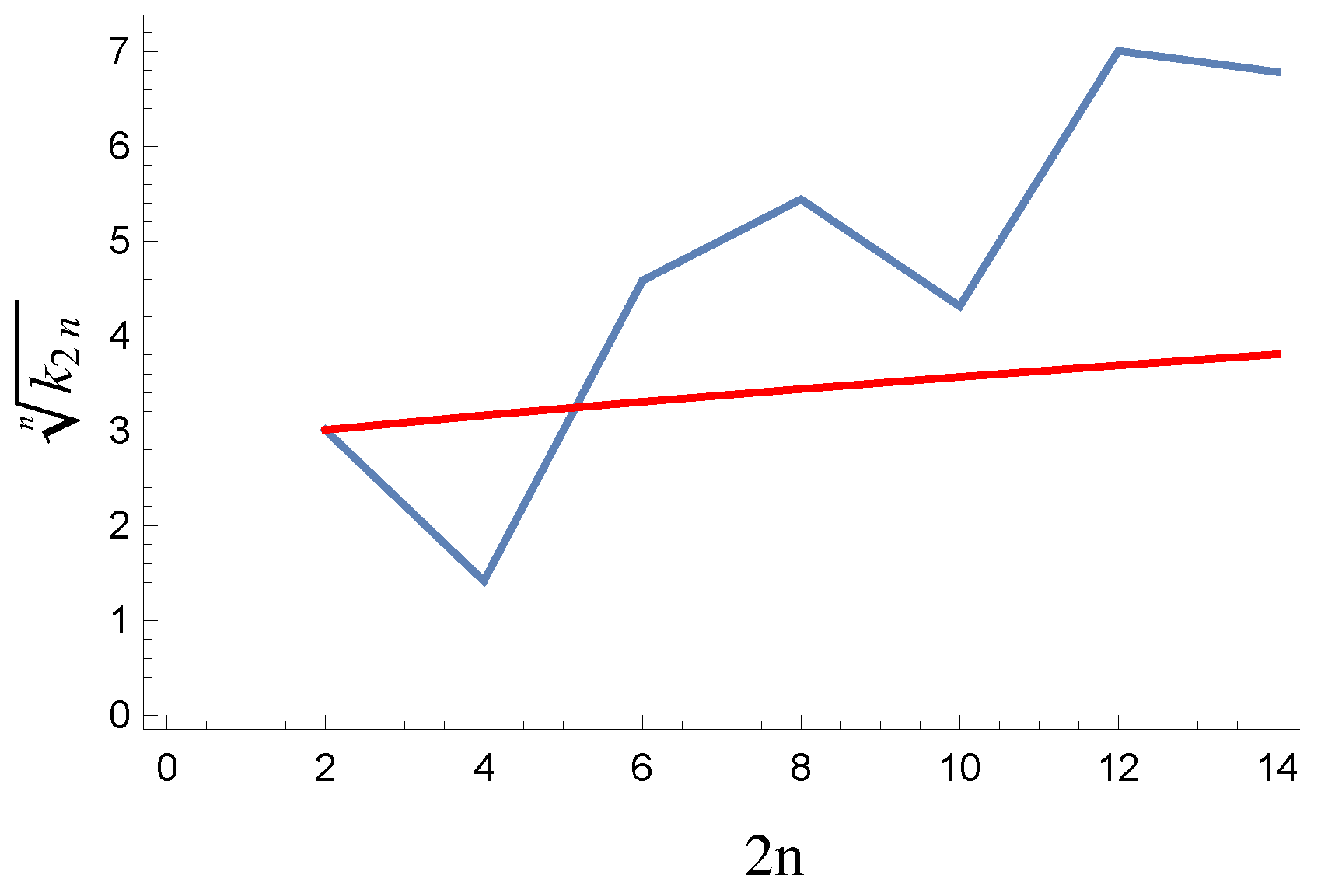
Figure 1. Schematic illustration of the scalar product (41)–(45).
Universe 09 00508 g001
Figure 2. n-th root of coefficient k 2 n in the expression < C | a ^ 2 n | C > = k 2 n η n for the mean value of the 2nth degree of scale factor with respect to the wave packet (21). The red and blue curves correspond to the etalon method and that with the Grassmann variables, respectively.
Universe 09 00508 g002
Table 1. The expectation values < C | a 2 n | C > = k 2 n η n for the wave packet (21).
2 n 2468101214
k 2 n n for the etalon model 16 3 π 10 64 π 3 140 4 1024 π 5 2520 6 20480 π 7
k 2 n n for the model with the Grassmann variables 16 3 π 2 512 3 π 3 876 4 7936 3 π 5 118280 6 1172480 π 7
Disclaimer/Publisher’s Note: The statements, opinions and data contained in all publications are solely those of the individual author(s) and contributor(s) and not of MDPI and/or the editor(s). MDPI and/or the editor(s) disclaim responsibility for any injury to people or property resulting from any ideas, methods, instructions or products referred to in the content.

