Abstract
To study the oscillations of active neutrinos in the framework of the model with three active and three sterile neutrinos, the analytical expressions are obtained for the appearance and survival probabilities of different neutrino flavors taking into account the decaying sterile neutrinos contributions. In the framework of the considered phenomenological neutrino model, we make an interpretation of the experimentally detected XENON1T-excess of electronic recoil events in the energy range of 1–7 keV as a result of the radiative decay of a sterile neutrino with a mass of about 7 keV. Estimations of the decay parameters for the radiative decay of Majorana sterile neutrinos due to the magnetic dipole transitions into the active neutrino states are made. The value of the parameter of active and sterile neutrinos mixing has been derived from the Baksan Experiment on Sterile Transitions (BEST) experimental data. The graphical dependences for the probabilities of appearance and survival of muonic and electron neutrinos at short baseline (SBL) are presented with the use of that gained from the experimental data estimations of the model parameters.
1. Introduction
As is known, the oscillations of solar, atmospheric, reactor, and accelerator active neutrinos can be described by mixing three mass neutrino states using the Pontecorvo–Maki–Nakagawa–Sakata matrix , with , where are left chiral fields with flavor a or mass , and . For three active neutrinos, the matrix V is expressed in the standard parametrization [1] through three mixing angles and the CP-phase associated with CP violation in the lepton sector for Dirac or Majorana neutrinos, while , where and are phases associated with CP violation only for Majorana neutrinos. At the present time, using experimental data, the mixing angles and the differences of the squared neutrino masses and are found [1,2,3] (where ), but the value of is still known only up to a sign. Therefore, the absolute values of the neutrino masses can be ordered in two ways, namely, as or as , which are called the normal order of neutrino masses (NO) or the inverse order of neutrino masses (IO), respectively. The use of non-zero neutrino masses leads to a Modified Standard Model (MSM) to replace the original Standard Model (SM) with zero neutrino masses. In what follows, we will consider only the NO-case of the neutrino mass spectrum at . Thus, our particular choice of the preferred mass ordering and the value is coming from recent experimental results (in particular, the results of the T2K experiment) [1,2].
Along with the measured standard oscillation data, the indications are obtained on anomalous data for neutrino fluxes in a number of processes that cannot be explained by using the oscillatory parameters for only three active neutrinos. These anomalies include LSND (or accelerating) anomaly (AA) [4,5,6], reactor antineutrino anomaly (RA) [7,8,9,10,11,12], and gallium (or calibration) anomaly (GA) [13,14,15,16,17,18]. Anomalies manifest themselves at small distances, more precisely, at such distances L from the source when the value of the parameter is of the order of unity, where E is the neutrino energy. AA, RA, and GA, that is, three types of neutrino anomalies on small (or short baseline (SBL)) distances, can be explained by the presence of at least one or two additional neutrinos that do not interact directly with gauge bosons of MSM; therefore, they are called sterile neutrinos (SN). The characteristic mass scale of SN that is suitable for explaining the SBL anomalies is 1 eV (see, for example, [19,20,21,22]).
In principle, the number of additional neutrinos can be arbitrary [23,24,25]. Phenomenological models containing SN are usually denoted as (3+N) models or, in more detail, as (k+3+n+m+...) models, where k is the number of new neutrinos with masses less than masses of active neutrinos, and n and m are the numbers of new neutrinos with masses large and significantly larger, respectively, than the masses of active neutrinos, etc. Properties of SN, if they really exist, have yet to be determined using experimental data and phenomenological models. For example, data from the XENON1T experiment were recently publiished that are related to electronic recoil events in the energy range between 1 keV and 210 keV [26], in which one can see an excess of electronic recoil events in the energy range between 1 keV and 7 keV compared to the calculated background. By now, a large number of works devoted to various options for explaining this effect have appeared (see, for example, [27,28,29,30,31,32,33,34]). In this work, we will hold to the interpretation of the observed effect as a result from sterile neutrino decays [31]. Thus, we take into account the possibility of decay of sterile neutrinos in the framework of the (3+3) neutrino model with three active and three sterile neutrinos [19]. This SN property allows us to explain the XENON1T-excess too, and for some values of the SN decay width, as is shown in this work, preserve the interpretation of SBL anomalies as an effect of sterile neutrinos. Note that such important characteristics of models with sterile neutrinos as mixing parameters of active and sterile neutrinos, obtained in different experiments in the framework of the simple (3+1) model, significantly disagree (see, for example, [35,36,37]). In the present work, we use the latest results of the Baksan Experiment on Sterile Transitions (BEST) [18] for estimating the value of the main mixing parameter of active and sterile neutrinos (parameter ) in the framework of the considered (3+3) model.
The paper is organized as follows: Section 2 contains the main propositions of the used (3+3) neutrino model, which are based on the results presented earlier in [19]. Section 3 provides a short description of data related to the excess of electronic recoil events in the XENON1T experiment and their interpretation within the framework of the used (3+3) model. In Section 4, analytical expressions for the appearance and survival probabilities for different flavors of stable and decaying neutrinos are given. In Section 5, the value of the main parameter related to the mixing of active and sterile neutrinos is obtained taking into account the last data of the experiment BEST. On the basis of the found values of the model parameters, the graphs of the appearance and survival probabilities of electron neutrinos and the survival probabilities of muon neutrinos are presented and discussed. In the final Section 6, it is noted that the results of this work can be used to interpret both the data obtained from the SBL experiments on the search for sterile neutrinos and the data from the XENON1T experiment, as well as some astrophysical data.
2. Phenomenological (3+3) Model of Neutrinos
Phenomenological neutrino (3+N) or (k+3+m+n+...) models are used to describe SBL anomalies as well as some astrophysical data, where is the number of additional neutrinos. Usually, models with a minimal number of N are used, such as (3+1) and (3+2) models [38]. In papers [39,40,41], taking into account left-right symmetry of weak interactions, the (3+3) model was considered, which will be used below. The (3+3) model includes three active neutrinos () and three new (sterile) neutrinos: light sterile neutrino , hidden neutrino , and dark neutrino [19]. Thus, this model contains six neutrino flavor states and six neutrino mass states. Therefore, to describe neutrino oscillations, it is necessary to use the generalized mixing matrix , which can be called the generalized Pontecorvo–Maki–Nakagawa–Sakata matrix . We represent as the matrix product , where P is a diagonal matrix containing the Majorana CP-phases , , that is, . Hereinafter, we will not use the general form of the matrix V, but employ only its particular forms. Preserving the continuity of notations, we denote the Dirac CP-phases as and , and the mixing angles as and , and, in doing so, , , and .
For compactness of formulas, we introduce symbols and for sterile left flavor fields and sterile left mass fields, respectively. Fields with index b contain fields , and , and will denote a set of indices 4, 5 and 6. A total 6 × 6 mixing matrix can be represented in terms of 3 × 3 matrices R, T, V, and W in the following way:
In the present state of the art, it is enough to restrict ourselves only to a minimal number of parameters of the mixing matrix , which allows interpretation of the available (still rather heterogeneous) experimental data. The transition to the full matrix with all parameters should be done later on, when reliable experimental results related to the revealed anomalies will be obtained. That is, only a few special cases of matrices R, T, V, and W are used below. Let us choose the matrix R in the form of , where and is a small value, while T in Equation (1), most likely, is a small matrix as compared to the well-known unitary mixing matrix of active neutrinos (). Thus, when choosing the appropriate normalization, the oscillations of active neutrinos are described, as it should be in MSM, with using the Pontecorvo–Maki–Nakagawa–Sakata matrix . Below the notation, will be used. Since, according to available astrophysical and laboratory data, the mixing between active and sterile neutrinos should be small, we choose matrix T in the form of , where a is an arbitrary unitary matrix (). In this case, the matrix can be written in the following form:
where b is also an arbitrary unitary matrix (), and . Under these conditions, the matrix will be unitary too (). Indeed, this structure of matrix is unambiguous, under the choice of matrix R as and from the requirement of its unitary. In particular, we will use the following matrices a and b:
where and are the mixing phases between active and sterile neutrinos, while and , as well as and are the mixing angles between them. Matrix a of the form (3a), but in the particular case at and , was used in the paper [41]. In some cases, it is desirable (as is seen below from the formula (8)) to have the values of the elements of the bottom (3rd) line of the resulting matrix with maximal modulus (for known fixed parameters and ). The remaining elements of the matrix are obtained in a standard way.
Let us specify the neutrino masses using a normally ordered set of values . For the masses of active neutrinos, we take the estimates of the neutrino masses proposed in [40,41,42] for the NO case (in units of eV), which do not contradict to up-to-date experimental data:
The values of mixing angles for active neutrinos, which define the Pontecorvo–Maki–Nakagawa–Sakata matrix, are calculated from the relations , and . These relations are obtained on the basis of processing of experimental data for the NO-case and are given in the paper [2]. Concrete values quoted above of masses and mixing angles for active neutrinos are within known experimental bounds [2]. The selection of these values is the admissible and convenient method of carrying out the following numerical calculations for the analysis of active neutrino oscillations at short baseline.
In the paper [19], a specific version of the (3+1+2) model was considered for the next values (in units of eV) of masses , , and (specified in [19] as the LMO1 option):
However, to reproduce the electron energy spectrum observed in the XENON1T experiment (in which, in the region of several keV, one can actually see one maximum at keV), and also taking into account the values of the SN masses used to explain MiniBooNE anomaly in [43], we will further use somewhat larger values of and masses than the corresponding mass values given in [19] and also above in the relations (5). To do this, let us take out from the keV range. It is necessary because only one maximum at keV has been observed in the XENON1T experiment. Thus, if one considers the radiative decays of (see Section 3), then the mass should be approximately equal to 7 keV. The value of the mass from the relations (5) is practically left unchanged (taking into account the experimental results of [18], its refined value is eV). This value of mass satisfies the current restrictions [44,45], but we note that for this work the change of its value in the square from eV up to 10 eV is not essential, and all of the following results substantially remain valid. Thus, in this paper, we will further use the following eV-values of the masses , , and :
Therefore, the considered (3+3) model is actually the (3+1+1+1) model. Note that sterile neutrinos in the mass range from 1 keV to 10 keV are currently being used to interpret some astrophysical data [46], which is consistent with our choice of mass equal to 7 keV.
To make the calculations more specific, we will use the following trial values of the new mixing parameters:
The general motivation for this choice is that the mixing between active and sterile neutrinos should be small, so that the mixing angles as well as the value of the parameter should not be quite large. However, for the crucial parameter responsible for the effects considered in the present paper, its model value was still fitted by visually comparing the oscillation curves of active neutrinos in the channels and (see Section 5). The value of the parameter will be found below in Section 5 using the experimental results of [18], which was obtained for the internal volume of the target filled with gallium.
3. The Excess of Electronic Recoil Events in the XENON1T Experiment and Its Interpretation in the Context of the (3+1+1+1) Model
The data from the XENON1T experiment on the observation of the excess of electronic recoil events in the energy range between 1 keV and 7 keV were presented recently [26]. The XENON1T experiment is being carried out underground in INFN National Laboratory in Gran Sasso. This experiment uses a time projection chamber filled by liquid xenon with a mass of the order of 1 ton. The experiment was originally intended to detect dark matter from weakly interacting massive particles (WIMP). Interaction of different particles inside the detector leads to the appearance of both fast scintillation signals and delayed electroluminescent signals. These light signals are detected by a system of photomultipliers above and below the working volume, and their readings determine the released energy and coordinates of events. The time relationship between electroluminescent signals and fast scintillation signals is used to determine electrons recoil that is produced, for example, by gamma rays or beta electrons, and which is compared with the nuclear recoil that is produced, for example, by neutrons or WIMPs. This procedure is essential for particle identification.
As a result of the measurements that have been carried out on determination of the number of electrons recoil events and subsequently comparing it with the background calculated for the given setup, the excess of such events was obtained in the region 1–7 keV with a maximum near 3 keV. If we take into account the additional contribution to the background due to tritium, then this maximum shifts to 3.5 keV [26]. Checking the detected anomaly will continue both in the XENON1T experiment and in future experiments of this type.
Let us dwell upon the possibility of a description of the electronic recoil event excess observed in the XENON1T experiment within the framework of the neutrino model considered in Section 2. We assume that this excess is due to the interaction of electrons with photons arising as a result of decays of hidden neutrinos that are captured by the Earth and are omnipresent in a laboratory with non-relativistic speeds, being in a dynamic equilibrium with dark matter particles and cosmic background neutrinos and photons [24,27,28,32,36,37]. Below, we will consider sterile neutrino decay mechanisms with a photon emission. Other possible decay mechanisms of hidden neutrinos, for example, with the help of dark bosons, are not being considered in this work due to their hypothetical nature [47,48].
First, let us consider and evaluate, in accordance with the method of the paper [49], the radiative decay widths of sterile neutrino mass states, which occur through the exchange by W-bosons and Higgs bosons. According to the results of [49], the decay width of the Majorana massive neutrino with mass into Majorana massive neutrino with mass under the condition can be approximately calculated by the formula:
where . For sterile neutrinos with masses of the order of several keV, an estimate of the width of their decay in energy units leads to an extremely small result eV (which corresponds to the estimate in time units as years ).
Therefore, let us consider other possible mechanisms of sterile neutrino decay [43], which can result in much larger decay widths. In Refs. [50,51,52], the interaction of neutrinos with an electromagnetic field due to anomalous dipole moments of neutrinos is considered (dipole portal). We restrict ourselves in this work to taking into account the magnetic dipole moments for decaying sterile neutrinos as Majorana particles. In this case, the intrinsic magnetic moments of SN are equal to zero, and nonzero are only off-diagonal matrix elements of the magnetic dipole moment (transient magnetic moments) responsible for electromagnetic transitions between different mass states of neutrinos [53]. Part of the Lagrangian, which contains the kinetic part of the Lagrangian of the electromagnetic field and also its interaction with anomalous magnetic moments of SN, has the form:
where
Then, due to the term with the interaction between neutrinos and photons in the formula (9), the decays of are possible. In particular, photons with energies approximately equal to keV, i.e., about one half of the neutrino mass, will be emitted from the decay of into the active neutrino mass states i (). Using the results of work [53], it is possible to relate the neutrino decay width due to such radiative decays with an effective transient magnetic moment of neutrinos:
where is the effective transition magnetic moment of heavy neutrino . To show the influence of decaying keV-range neutrino on oscillation characteristics of active neutrinos, we will use the phenomenological value of the decay width eV, which in time units corresponds to the value c . This value of allows us to conserve the oscillations of active neutrinos with a small effect from decay. Then, for the mass value keV, it is possible to obtain from relation (11) that it corresponds to the value of the effective transient magnetic moment of neutrino of the order of . For massive neutrino , if its width is eV, it must have the effective transient magnetic moment ∼. At the same time, even if the transient magnetic moment of a light sterile neutrino estimates by a value of the order of (or less), then the width of its decay due to a magnetic-dipole interaction should not exceed the rather small value eV. In this paper, we do not consider other possible mechanisms leading in some cases to sufficiently large values of , which may also include the contributions of interactions in the dark sector.
4. Analytical Expressions for the Appearance and Survival Probabilities of Neutrino Flavors
In this section, we present a generalization of the analytical expressions for the probabilities of transitions and conservations of various neutrino flavors, which were obtained in Ref. [25] in the case of stable neutrinos, to the case of decaying neutrinos. Using equations for propagation of various neutrino flavors (see, for example, [19]), it is possible to obtain analytical expressions for the transition probabilities of various flavors of stable neutrinos/antineutrinos in a vacuum as a function of distance L from neutrino source. If is a generalized mixing matrix in the form of expression (2), and if one uses notation , then, following [25], it is possible to calculate the transition probabilities from to , or from to by the formula
where the upper sign corresponds to neutrino transitions while the undersign corresponds to antineutrino transitions . Note that the flavor indices and (as well as the summation indices i and k over mass states) are applied to all neutrinos, that is, to active and sterile neutrinos. Moreover, as follows from the Equation (12), the relation is fulfilled exactly due to the CPT-invariance condition [25].
The expressions (12) given above are directly generalized to the case of decaying neutrinos with allowance for their decay widths for the k-th neutrino mass state. For this, in the original equations for propagation of neutrino flavors [19], it is necessary to substitute the complex quantity instead of neutrino energy , that in a result permits us to take into account a possibility of decay with a decay width for any k-th mass neutrino state. Then, the probabilities of transitions from to , or from to , will be calculated as follows:
where . The upper sign corresponds to neutrino transitions , and the lower sign corresponds to antineutrino transitions . For this, is equivalent to , if is given in eV, E is given in MeV, and L is given in meters. Respectively, is equivalent to , if L is given in meters, and and are given in eV.
5. Evaluation of Mixing of Light and Heavy Neutrinos by the BEST Experimental Result and Calculations of the Appearance and Survival Probabilities for Active Neutrinos
Let us now estimate the value of the parameter for the mixing matrix , with using the experimental result [18] obtained for the internal volume of a target in the form of a sphere filled with gallium. This experiment uses neutrino radiation from radioactive Cr to calibrate the detector. The spectrum of Cr is well known and consists of two dominant monoenergetic components and two subdominant monoenergetic components. The source with Cr is placed in a cylinder, which is in turn inserted into a sphere filled with gallium. This sphere forms the inner target volume, while the outer volume consists of a large cylinder also filled with gallium. The inner radius of the sphere is cm, and a cylinder with a radius of about cm is inserted into this sphere, so one end of this cylinder is cm below the center of the sphere, while the other end of the cylinder reaches the edge of the sphere. Integrating over the interior of the sphere without a cylinder, first with probability according to the formula (13), then with a unit probability, and, taking the ratio of the results obtained, we obtain the value of the averaged value , which, according to [18], should be equal to . In this, with sufficient accuracy, the influence of the cylinder can be neglected, the proportion of which in the working volume is less than . It should be also taken into account that electron neutrinos in cases are emitted with an energy of 747 keV, in cases, they are emitted with an energy of 427 keV, in cases, they are emitted with an energy of 752 keV and, in cases, they are emitted with an energy of 432 keV. After the performed calculations, the estimate of the value of the parameter is 0.087, if we use value .
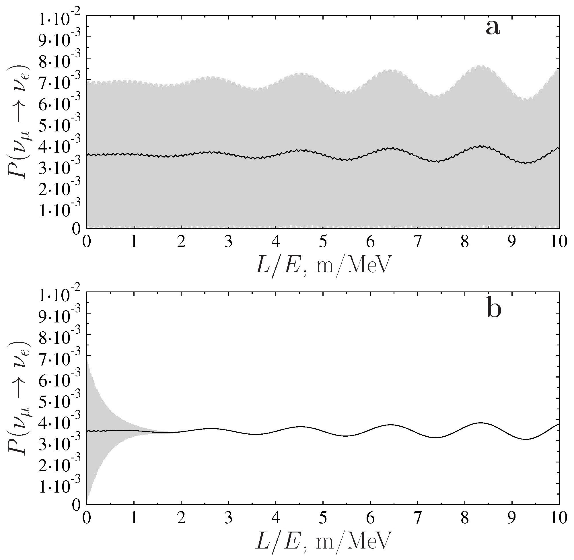
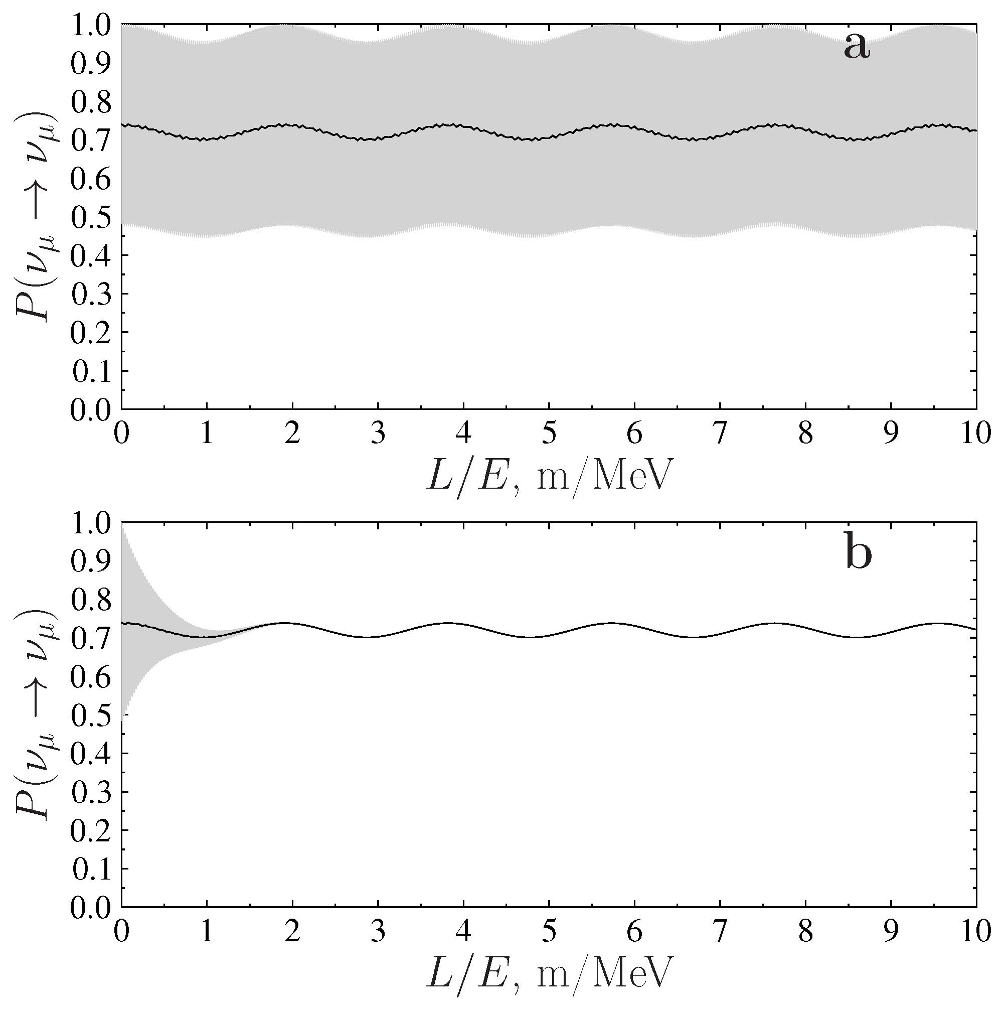
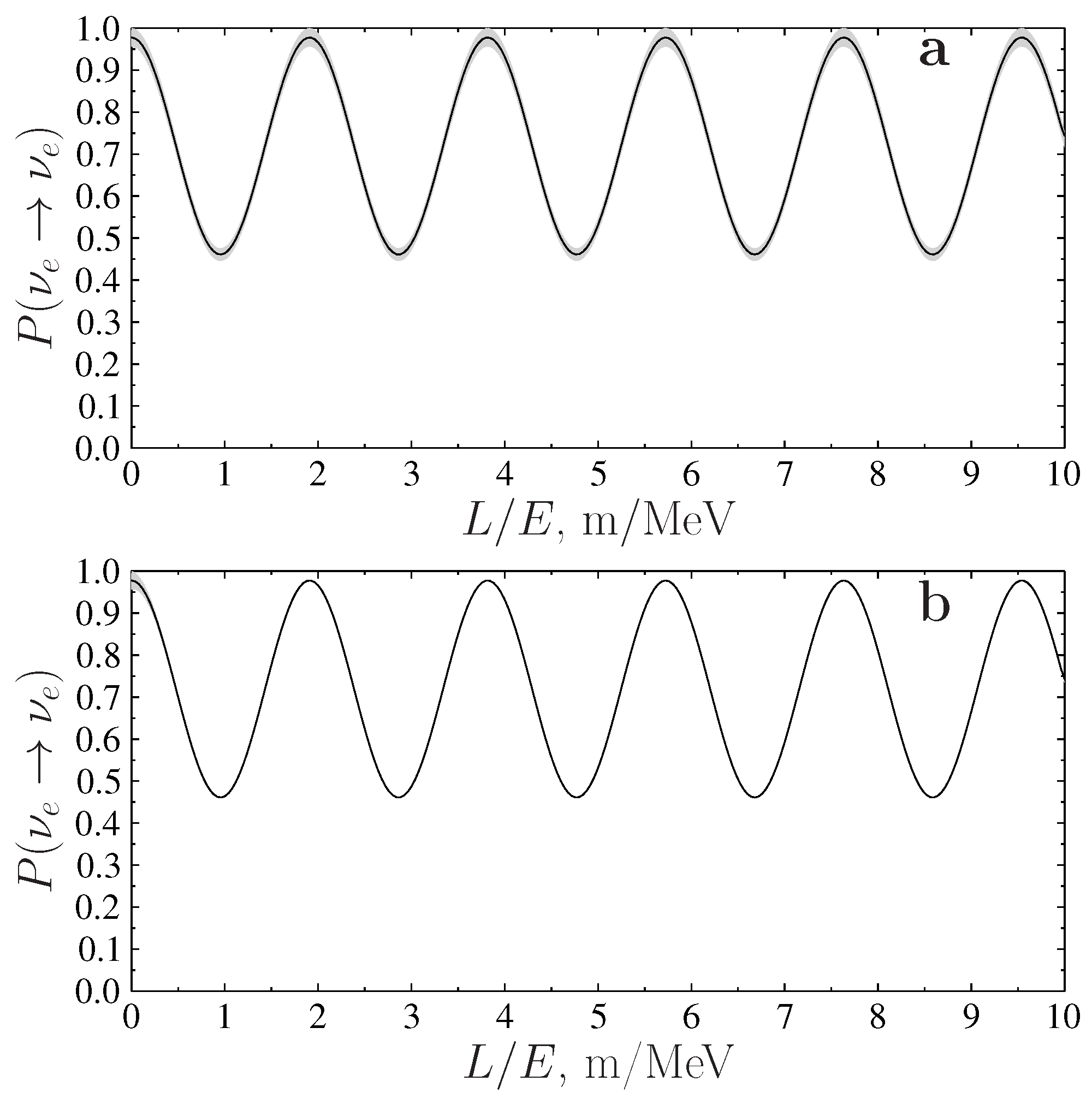
Now, one can plot the appearance and survival probabilities for various neutrino flavors in the considered model. Figure 1 shows the probabilities of appearance of (a and b) as a function of the ratio of the distance L from the source to the neutrino energy E in the beams of for stable (a) and decaying (b) sterile neutrinos for the neutrino mass spectrum considered in this paper and for the decay widths of sterile neutrinos eV, eV and eV. Motivation for the choice of such test values for decaying widths of sterile neutrino states is given in Section 3, and, for the matrix , the values and were taken. The value of was obtained above in this section based on the result of work [18]. Furthermore, in all the figures, the gray area corresponds to the exact calculations of fast oscillations caused by the presence in the model of the fifth keV-range neutrino, while the solid line shows probability values averaged over a small spatial scale. In Figure 2, similar results for stable (a) and decaying (b) sterile neutrinos are given for for the same model parameter values. Figure 3 shows similar results for stable (a) and decaying (b) sterile neutrinos for .
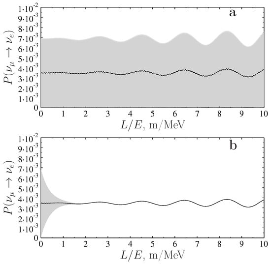
Figure 1.
The probability of appearance of depending on the ratio of the distance L from the source to the neutrino energy E in the beams of for stable (a) and decaying (b) sterile neutrinos with masses eV, keV and MeV and with decay widths eV, eV and eV. For matrix , and ( and ).
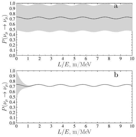
Figure 2.
The survival probabilities for depending on the ratio of the distance L from the source to the neutrino energy E in the beams of for stable (a) and decaying (b) sterile neutrinos with masses eV, keV and MeV and with decay widths eV, eV and eV. For matrix , and ( and ).
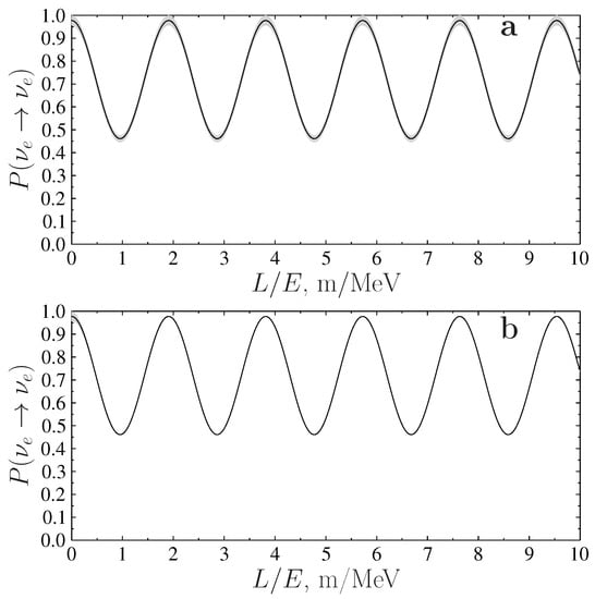
Figure 3.
The survival probabilities for depending on the ratio of the distance L from the source to the neutrino energy E in the beams of for stable (a) and decaying (b) sterile neutrinos with masses eV, keV and MeV and with decay widths eV, eV and eV. For matrix , and ( and ).
As can be seen from the results presented in these figures, the very small width of light sterile neutrino has practically no effect on oscillation characteristics of active neutrinos. However, the width of of a keV-range neutrino already affects fast oscillations from keV-range sterile neutrinos, which are visually represented by a gray background in Figure 1, Figure 2 and Figure 3. As a result, for excluding the initial part of small values of the ratio, the contribution of sterile neutrinos has the character of smooth oscillations corresponding to oscillations on smooth averaged curves in Figure 1a, Figure 2a and Figure 3a for stable sterile neutrinos. These oscillations in the range of values m/MeV are less pronounced in the initial part for accelerating anomaly corresponding to Figure 1, but it remains clearly expressed for reactor and calibration anomalies, which gives these anomalies preference for research on the search for sterile neutrinos.
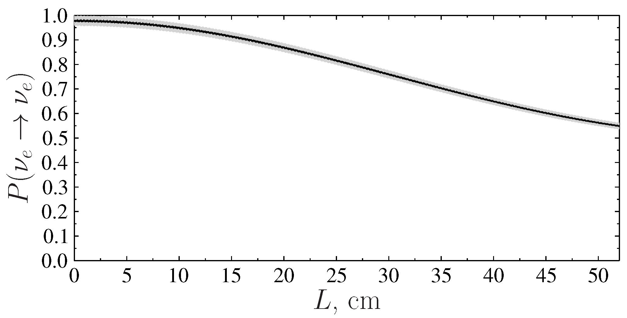
In Figure 4, the survival probability for electron neutrinos as a function of distance L from the source is shown specifically for the conditions of the BEST experiment corresponding to the experimental value for the values of the model parameters and . When decreasing the value of , the parameter will increase, while the influence of a light sterile neutrino in the channel will decrease more.

Figure 4.
The survival probabilities for depending on the distance L from the neutrino source with parameter values and for the conditions of the Baksan Experiment on Sterile Transitions (BEST) [18].
Thus, with mass values from Equations (4) and (6) for active and sterile neutrinos given in Section 2, respectively, it remains possible to interpret the neutrino data anomalies at small distances [54,55] as the sterile neutrino effect in the case of decaying sterile neutrinos [31] (see Figure 1, Figure 2 and Figure 3) provided that the largest period of oscillations among sterile neutrinos is much less than the smallest half-life among these sterile neutrinos. In this work, we focus principally on how the presence of decay widths of decaying sterile neutrinos can affect the oscillatory characteristics of active neutrinos. A comparison of the results of our model with the results of a simple (3+1) model, which are obtained on the basis of available experimental data, was made in Ref. [19] and shows that it is most probably that all SBL anomalies data cannot be described with the usual simple formula of the (3+1) model depending on the same value of characteristic parameter .
6. Discussion and Conclusions
In this paper, the phenomenological (3+3) neutrino model with three active neutrinos and three decaying sterile neutrinos is used for a description of oscillations of active neutrinos at small distances. Generalization of formulas for the probabilities of appearance and survival of various neutrino flavors taking into account the contributions of decaying neutrinos is obtained. In addition, estimates are made for some parameters of the used model, which are based on the latest XENON1T and BEST experimental data, and the test parameter values are chosen when the experimental data are not known well enough. With the selected parameter values, the calculations of the probabilities are made, and the corresponding figures are presented taking into account the contributions of decaying sterile neutrinos (Figure 1, Figure 2 and Figure 3). Suppression of oscillations due to decaying light sterile neutrinos turns out to be insignificant, but the decay of keV-range neutrino suppresses fast oscillations associated with this neutrino state, and, for the reactor and gallium anomalies, the oscillations are quite pronounced practically over the entire range of values m/MeV. Since the most predictable theoretical dependence of the neutrino spectrum on is known namely for the gallium anomaly (as is known, there are still problems with calculating the fluxes of reactor antineutrinos and comparing their values with really existing ones (see, for example, [56,57,58,59])), thus the experimental confirmation of this anomaly at the level obtained in the experiment BEST [18] is of great importance. Using the results of [18], the value of the mass of the light sterile neutrino was refined, and the value of the parameter for the mixing matrix , which is the main parameter of mixing between light and heavy neutrinos in the considered (3+3) model, was evaluated. At the same time, note that, although first MicroBooNE results do not confirm the MiniBooNE results for acceleration anomaly (AA), they do not exclude the possible existence of a light sterile neutrino [60].
The exclusion of the existence of a light sterile neutrino can follow from data for the effective number of relativistic particles , which contribute to the total amount of radiation in the early Universe. If light sterile neutrinos are in complete thermal equilibrium with other relativistic particles, then . Thus, light sterile neutrinos can not be in complete thermal equilibrium either due to the small mixing between active and sterile neutrinos or due to non-standard neutrino interactions, or for both reasons (see, for example, [61])—insofar as conclusions drawn from astrophysical or cosmological data depend on the models and datasets used, so in some cases changing the dataset or the model can lead to a different result, in particular, for .
In this work, the excess of electronic recoil events in the energy range of 1–7 keV found in the data of the XENON1T experiment [26] is interpreted as the result of the interaction of electrons with photons, which are emitted during the decays of sterile mass states. In this case, the decay of a sterile state with mass ∼7 keV into the active neutrino states with masses () leads to the appearance of an almost aggregate peak at keV for electronic recoil events. Such a consequence of the adopted interpretation is consistent with available data from XENON1T and can be verified both in the ongoing XENON1T experiment and in future experiments, such as XENONnT [26] and LZ [62].
If we assume that, thanks to the results of further observations, the existence of three sterile neutrinos will be confirmed, then it can lead to a significant change in the interpretation of a number of phenomena both in neutrino physics and in astrophysics. For example, it becomes possible to explain neutrino data on short distances for the gallium anomaly, as well as the appearance of a line near keV in gamma spectra of a number of astrophysical sources. As is shown in this work, to describe the SBL neutrino anomalies, the variant of a (3+3) neutrino model given by Equation (6) with decaying sterile neutrinos is applicable (see Figure 1, Figure 2 and Figure 3). At the same time, these figures also show that the procedure for determining the mass of the lightest sterile neutrino on the base of the data of accelerator experiments at on the order of 1 m/MeV can be ambiguous, and the results may not agree with the results obtained for the gallium anomaly. This means that a simple (3+1) neutrino model with a stable light sterile neutrino can be poorly applicable for a general (global) description of the valuable data for all SBL neutrino anomalies. At the same time, the (3+3) neutrino model with decaying sterile neutrinos, which is considered in the present paper, is a suitable working scheme for the interpretation and description of available SBL neutrino data, as well as some astrophysical observations.
Author Contributions
The authors contributed equally to this work. Conceptualization, V.K. and S.F.; methodology, V.K. and S.F.; validation, S.F. and V.K.; software, S.F. and V.K.; formal analysis, V.K. and S.F.; investigation, S.F. and V.K.; writing—original draft preparation, V.K. and S.F.; writing—review and editing, S.F. and V.K. All authors have read and agreed to the published version of the manuscript.
Funding
This research received no external funding.
Institutional Review Board Statement
Not applicable.
Informed Consent Statement
Not applicable.
Data Availability Statement
Not applicable.
Acknowledgments
We are grateful to three anonymous reviewers for the excellent feedback we received.
Conflicts of Interest
The authors declare no conflict of interest.
References
- Particle Data Group; Zyla, P.A.; Barnett, R.M.; Beringer, J.; Dahl, O.; Dwyer, D.A.; Groom, D.E.; Lin, C.-J.; Lugovsky, K.S.; Pianori, E.; et al. The Review of Particle Physics. Prog. Theor. Exp. Phys. 2020, 2020, 083C01. Available online: https://pdg.lbl.gov/ (accessed on 23 December 2021).
- De Salas, P.F.; Forero, D.V.; Gariazzo, S.; Martínez-Miravé, P.; Mena, O.; Ternes, C.A.; Tórtola, M.; Valle, J.W.F. 2020 global reassessment of the neutrino oscillation picture. J. High Energy Phys. 2021, 2102, 071. [Google Scholar] [CrossRef]
- Hu, Z.; Ling, J.; Tang, J.; Wang, T.-C. Global oscillation data analysis on the 3ν mixing without unitarity. J. High Energy Phys. 2021, 2101, 124. [Google Scholar] [CrossRef]
- Athanassopoulos, C.; Auerbach, L.B.; Burman, R.L.; Cohen, I.; Caldwell, D.O.; Dieterle, B.D.; Donahue, J.B.; Eisner, A.M.; Fazely, A.; Federspiel, F.J.; et al. Evidence for → oscillations from the LSND experiment at the Los Alamos Meson Physics Facility. Phys. Rev. Lett. 1996, 77, 3082. [Google Scholar] [CrossRef] [PubMed] [Green Version]
- Aguilar, A.; Auerbach, L.B.; Burman, R.L.; Caldwell, D.O.; Church, E.D.; Cochran, A.K.; Donahue, J.B.; Fazely, A.; Garvey, G.T.; Gunasingha, R.M.; et al. Evidence for neutrino oscillations from the observation of appearance in a beam. Phys. Rev. D 2001, 64, 112007. [Google Scholar] [CrossRef] [Green Version]
- Aguilar-Arevalo, A.A.; Brown, B.C.; Conrad, J.M.; Dharmapalan, R.; Diaz, A.; Djurcic, Z.; Finley, D.A.; Ford, R.; Garvey, G.T.; Gollapinni, S.; et al. Updated MiniBooNE neutrino oscillation results with increased data and new background studies. Phys. Rev. D 2021, 103, 052002. [Google Scholar] [CrossRef]
- Mueller, T.; Lhuillier, D.; Fallot, M.; Letourneau, A.; Cormon, S.; Fechner, M.; Giot, L.; Lasserre, T.; Martino, J.; Mention, G.; et al. Improved predictions of reactor antineutrino spectra. Phys. Rev. C 2011, 83, 054615. [Google Scholar] [CrossRef] [Green Version]
- Mention, G.; Fechner, M.; Lasserre, T.; Mueller, T.A.; Lhuillier, D.; Cribier, M.; Letourneau, A. Reactor antineutrino anomaly. Phys. Rev. D 2011, 83, 073006. [Google Scholar] [CrossRef] [Green Version]
- Huber, P. Determination of antineutrino spectra from nuclear reactors. Phys. Rev. C 2011, 84, 024617, Erratum in Phys. Rev. C 2012, 85, 029901. [Google Scholar] [CrossRef] [Green Version]
- Ko, Y.J.; Kim, B.R.; Kim, J.Y.; Han, B.Y.; Jang, C.H.; Jeon, E.J.; Joo, K.K.; Kim, H.J.; Kim, H.S.; Kim, Y.D.; et al. Sterile neutrino search at the NEOS experiment. Phys. Rev. Lett. 2017, 118, 121802. [Google Scholar] [CrossRef] [Green Version]
- Alekseev, I.; Belov, V.; Brudanin, V.; Danilov, M.; Egorov, V.; Filosofov, D.; Fomina, M.; Hons, Z.; Kazartsev, S.; Kobyakin, A.; et al. Search for sterile neutrinos at the DANSS experiment. Phys. Lett. B 2018, 787, 56. [Google Scholar] [CrossRef]
- Serebrov, A.P.; Samoilov, R.M.; Ivochkin, V.G.; Fomin, A.K.; Zinoviev, V.G.; Neustroev, P.V.; Golovtsov, V.L.; Volkov, S.S.; Chernyj, A.V.; Zherebtsov, O.M.; et al. Search for sterile neutrinos with the Neutrino-4 experiment and measurement results. Phys. Rev. D 2021, 104, 032003. [Google Scholar] [CrossRef]
- Hampel, W.; Heusser, G.; Kiko, J.; Kirsten, T.; Laubenstein, M.; Pernicka, E.; Rau, W.; Rönn, U.; Schlosser, C.; Wójcik, M.; et al. Final results of the 51Cr neutrino source experiments in GALLEX. Phys. Lett. B 1998, 420, 114–126. [Google Scholar] [CrossRef] [Green Version]
- Abdurashitov, J.N.; Gavrin, V.N.; Girin, S.V.; Gorbachev, V.V.; Gurkina, P.P.; Ibragimova, T.V.; Kalikhov, A.V.; Khairnasov, N.G.; Knodel, T.V.; Matveev, V.A.; et al. Measurement of the response of a Ga solar neutrino experiment to neutrinos from a 37Ar source. Phys. Rev. C 2006, 73, 045805. [Google Scholar] [CrossRef] [Green Version]
- Abdurashitov, J.N.; Gavrin, V.N.; Gorbachev, V.V.; Gurkina, P.P.; Ibragimova, T.V.; Kalikhov, A.V.; Khairnasov, N.G.; Knodel, T.V.; Mirmov, I.N.; Shikhin, A.A.; et al. Measurement of the solar neutrino capture rate with gallium metal. III. Results for the 2002–2007 data-taking period. Phys. Rev. C 2009, 80, 015807. [Google Scholar] [CrossRef]
- Kaether, F.; Hampel, W.; Heusser, G.; Kiko, J.; Kirsten, T. Reanalysis of the Gallex solar neutrino flux and source experiments. Phys. Lett. B 2010, 685, 47. [Google Scholar] [CrossRef] [Green Version]
- Giunti, C.; Laveder, M.; Li, Y.F.; Long, H.W. Pragmatic view of short-baseline neutrino oscillations. Phys. Rev. D 2013, 88, 073008. [Google Scholar] [CrossRef] [Green Version]
- Barinov, V.V.; Cleveland, B.T.; Danshin, S.N.; Ejiri, H.; Elliott, S.R.; Frekers, D.; Gavrin, V.N.; Gorbachev, V.V.; Gorbunov, D.S.; Haxton, W.C.; et al. Results from the Baksan Experiment on Sterile Transitions (BEST). arXiv 2021, arXiv:2109.11482. [Google Scholar]
- Khruschov, V.V.; Fomichev, S.V. Sterile neutrinos influence on oscillation characteristics of active neutrinos at short distances in the generalized model of neutrino mixing. Int. J. Mod. Phys. A 2019, 34, 1950175. [Google Scholar] [CrossRef] [Green Version]
- Dentler, M.; Esteban, I.; Kopp, J.; Machado, P. Decaying sterile neutrinos and the short baseline oscillation anomalies. Phys. Rev. D 2020, 101, 115013. [Google Scholar] [CrossRef]
- De Gouvêa, A.; Peres, O.L.G.; Prakash, S.; Stenico, G.V. On the decaying-sterile-neutrino solution to the electron (anti)neutrino appearance anomalies. J. High Energy Phys. 2020, 2007, 141. [Google Scholar] [CrossRef]
- Abdullahi, A.; Denton, P.B. Visible decay of astrophysical neutrinos at IceCube. Phys. Rev. D 2020, 102, 023018. [Google Scholar] [CrossRef]
- Bilenky, S.M.; Pontekorvo, B.M. Lepton mixing and neutrino oscillations. Sov. Phys. Usp. 1977, 20, 776–795. [Google Scholar] [CrossRef]
- Abazajian, K.N.; Acero, M.A.; Agarwalla, S.K.; Aguilar-Arevalo, A.A.; Albright, C.H.; Antusch, S.; Argüelles, C.A.; Balantekin, A.B.; Barenboim, G.; Barger, V.; et al. Light sterile neutrinos: A white paper. arXiv 2012, arXiv:1204.5379. [Google Scholar]
- Bilenky, S.M. Some comments on high precision study of neutrino oscillations. Phys. Part. Nucl. Lett. 2015, 12, 453–461. [Google Scholar] [CrossRef] [Green Version]
- Aprile, E.; Aalbers, J.; Agostini, F.; Alfonsi, M.; Althueser, L.; Amaro, F.D.; Antochi, V.C.; Angelino, E.; Angevaare, J.R.; Arneodo, F.; et al. Excess electronic recoil events in XENON1T. Phys. Rev. D 2020, 102, 072004. [Google Scholar] [CrossRef]
- Bell, N.F.; Dent, J.B.; Dutta, B.; Ghosh, S.; Kumar, J.; Newstead, J.L. Explaining the XENON1T excess with luminous dark matter. Phys. Rev. Lett. 2020, 125, 161803. [Google Scholar] [CrossRef]
- Choi, G.; Suzuki, M.; Yanagida, T.T. XENON1T anomaly and its implication for decaying warm dark matter. Phys. Lett. B 2020, 811, 135976. [Google Scholar] [CrossRef]
- Lindner, M.; Mambrini, Y.; de Melo, T.B.; Queiroz, F.S. XENON1T anomaly: A light Z′ from a two Higgs doublet model. Phys. Lett. B 2020, 811, 135972. [Google Scholar] [CrossRef]
- Ge, S.-F.; Pasquini, P.; Sheng, J. Solar neutrino scattering with electron into massive sterile neutrino. Phys. Lett. B 2020, 810, 135787. [Google Scholar] [CrossRef]
- Khruschov, V.V. Interpretation of the XENON1T excess in the model with decaying sterile neutrinos. arXiv 2021, arXiv:2008.03150v2. [Google Scholar]
- Aboubrahim, A.; Klasen, M.; Nath, P. Xenon-1T excess as a possible signal of a sub-GeV hidden sector dark matter. arXiv 2020, arXiv:2011.08053. [Google Scholar] [CrossRef]
- Chiang, C.-W.; Lu, B.-Q. Evidence of a simple dark sector from XENON1T excess. Phys. Rev. D 2020, 102, 123006. [Google Scholar] [CrossRef]
- Arcadi, G.; Bally, A.; Goertz, F.; Tame-Narvaez, K.; Tenorth, V.; Vogl, S. EFT interpretation of XENON1T electron recoil excess: Neutrinos and dark matter. Phys. Rev. D 2021, 103, 023024. [Google Scholar] [CrossRef]
- Machado, P.A.N.; Palamara, O.; Schmitz, D.W. The short-baseline neutrino program at Fermilab. Ann. Rev. Nucl. Part. Sci. 2019, 69, 363–387. [Google Scholar] [CrossRef] [Green Version]
- Diaz, A.; Argüelles, C.A.; Collin, G.H.; Conrad, J.M.; Shaevitz, M.H. Where are we with light sterile neutrinos? Phys. Rep. 2020, 884, 1–59. [Google Scholar] [CrossRef]
- Argüelles, C.A.; Aurisano, A.J.; Batell, B.; Berger, J.; Bishai, M.; Boschi, T.; Byrnes, N.; Chatterjee, A.; Chodos, A.; Coan, T.; et al. New opportunities at the next-generation neutrino experiments I: BSM neutrino physics and dark matter. Rept. Prog. Phys. 2020, 83, 124201. [Google Scholar] [CrossRef]
- Kopp, J.; Machado, P.A.N.; Maltoni, M.; Schwetz, T. Sterile neutrino oscillations: The global picture. J. High Energy Phys. 2013, 1305, 050. [Google Scholar] [CrossRef] [Green Version]
- Conrad, J.M.; Ignarra, C.M.; Karagiorgi, G.; Shaevitz, M.H.; Spitz, J. Sterile neutrino fits to short-baseline neutrino oscillation measurements. Adv. High Energy Phys. 2013, 2013, 163897. [Google Scholar] [CrossRef] [Green Version]
- Zysina, N.Y.; Fomichev, S.V.; Khruschov, V.V. Mass properties of active and sterile neutrinos in a phenomenological (3+1+2) model. Phys. Atom. Nucl. 2014, 77, 890–900. [Google Scholar] [CrossRef]
- Khruschov, V.V.; Fomichev, S.V.; Titov, O.A. Oscillation properties of active and sterile neutrinos and neutrino anomalies at short distances. Phys. Atom. Nucl. 2016, 79, 708–720. [Google Scholar] [CrossRef] [Green Version]
- Yudin, A.V.; Nadyozhin, D.K.; Khruschov, V.V.; Fomichev, S.V. Neutrino fluxes from a core-collapse supernova in a model with three sterile neutrinos. Astron. Lett. 2016, 42, 800–814. [Google Scholar] [CrossRef] [Green Version]
- Vergani, S.; Kamp, N.W.; Diaz, A.; Argüelles, C.A.; Conrad, J.M.; Shaevitz, M.H.; Uchida, M.A. Explaining the MiniBooNE excess through a mixed model of neutrino oscillation and decay. Phys. Rev. D 2021, 104, 095005. [Google Scholar] [CrossRef]
- Archidiacono, M.; Gariazzo, S.; Giunti, C.; Hannestad, S.; Tram, T. Sterile neutrino self-interactions: H0 tension and short-baseline anomalies. J. Cosmol. Astropart. Phys. 2020, 2012, 029. [Google Scholar] [CrossRef]
- Vagnozzi, S. New physics in light of the H0 tension: An alternative view. Phys. Rev. D 2020, 102, 023518. [Google Scholar] [CrossRef]
- Schneider, A. Constraining noncold dark matter models with the global 21-cm signal. Phys. Rev. D 2018, 98, 063021. [Google Scholar] [CrossRef] [Green Version]
- Arias, P.; Cadamuro, D.; Goodsell, M.; Jaeckel, J.; Redondo, J.; Ringwald, A. WISPy cold dark matter. J. Cosmol. Astropart. Phys. 2012, 1206, 013. [Google Scholar] [CrossRef]
- Brito, R.; Grillo, S.; Pani, P. Black hole superradiant instability from ultralight spin-2 fields. Phys. Rev. Lett. 2020, 124, 211101. [Google Scholar] [CrossRef]
- Pal, P.B.; Wolfenstein, L. Radiative decays of massive neutrinos. Phys. Rev. D 1982, 25, 766–773. [Google Scholar] [CrossRef]
- Palomares-Ruiz, S.; Pascoli, S.; Schwetz, T. Explaining LSND by a decaying sterile neutrino. J. High Energy Phys. 2005, 0509, 048. [Google Scholar] [CrossRef] [Green Version]
- Masip, M.; Masjuan, P.; Meloni, D. Heavy neutrino decays at MiniBooNE. J. High Energy Phys. 2013, 1301, 106. [Google Scholar] [CrossRef] [Green Version]
- Magill, G.; Plestid, R.; Pospelov, M.; Tsai, Y.-D. Dipole portal to heavy neutral leptons. Phys. Rev. D 2018, 98, 115015. [Google Scholar] [CrossRef] [Green Version]
- Giunti, C.; Studenikin, A. Neutrino electromagnetic interactions: A window to new physics. Rev. Mod. Phys. 2015, 87, 531–591. [Google Scholar] [CrossRef] [Green Version]
- Gariazzo, S.; Giunti, C.; Laveder, M.; Li, Y.F. Updated global 3+1 analysis of short-baseline neutrino oscillations. J. High Energy Phys. 2017, 1706, 135. [Google Scholar] [CrossRef] [Green Version]
- Palazzo, A. Exploring light sterile neutrinos at long baseline experiments: A review. Universe 2020, 6, 41. [Google Scholar] [CrossRef] [Green Version]
- Kopeikin, V.; Skorokhvatov, M.; Titov, O. Reevaluating reactor antineutrino spectra with new measurements of the ratio between 235U and 239Pu β Spectra. Phys. Rev. D 2021, 104, L071301. [Google Scholar] [CrossRef]
- Lyashuk, V.I. Problem of reactor antineutrino spectrum errors and its alternative solution in the regulated spectrum scheme. Results Phys. 2017, 7, 1212–1213. [Google Scholar] [CrossRef]
- Antonelli, V.; Miramonti, L.; Ranucci, G. Present and future contributions of reactor experiments to mass ordering and neutrino oscillation studies. Universe 2020, 6, 52. [Google Scholar] [CrossRef] [Green Version]
- Naumov, V.A.; Shkirmanov, D.S. Reactor antineutrino anomaly reanalysis in context of inverse-Square law violation. Universe 2021, 7, 246. [Google Scholar] [CrossRef]
- Denton, P.B. Sterile neutrino searches with MicroBooNE: Electron neutrino disappearance. arXiv 2021, arXiv:2111.05793. [Google Scholar]
- Gariazzo, S. Light sterile neutrinos. arXiv 2021, arXiv:2110.09876v2. [Google Scholar] [CrossRef] [Green Version]
- Akerib, D.; Akerlof, C.; Akimov, D.; Alquahtani, A.; Alsum, S.; Anderson, T.; Angelides, N.; Araújo, H.; Arbuckle, A.; Armstrong, J.; et al. The LUX-ZEPLIN (LZ) experiment. Nucl. Inst. Methods in Phys. Res. A 2020, 953, 163047. [Google Scholar] [CrossRef] [Green Version]
Publisher’s Note: MDPI stays neutral with regard to jurisdictional claims in published maps and institutional affiliations. |
© 2022 by the authors. Licensee MDPI, Basel, Switzerland. This article is an open access article distributed under the terms and conditions of the Creative Commons Attribution (CC BY) license (https://creativecommons.org/licenses/by/4.0/).