Observation of Atmospheric Neutrinos


Experimental Particle Physics Group, Department of Physics, Okayama University, Okayama 7008530, Japan
Universe 2020, 6(6), 80; https://doi.org/10.3390/universe6060080
Submission received: 21 April 2020
/
Revised: 1 June 2020
/
Accepted: 1 June 2020
/
Published: 5 June 2020
(This article belongs to the Special Issue Neutrino Oscillations)
Abstract
In 1998, the Super-Kamiokande discovered neutrino oscillation using atmospheric neutrino anomalies. It was the first direct evidence of neutrino mass and the first phenomenon to be discovered beyond the standard model of particle physics. Recently, more precise measurements of neutrino oscillation parameters using atmospheric neutrinos have been achieved by several detectors, such as Super-Kamiokande, IceCube, and ANTARES. In addition, precise predictions and measurements of atmospheric neutrino flux have been performed. This paper presents the history, current status, and future prospects of the atmospheric neutrino observation.
1. Introduction
1.1. History
Atmospheric neutrinos are generated when primary cosmic rays strike nuclei in the atmosphere and the hadron that results from these collision decays [1]. The principles and expected event rates of neutrino detection were first proposed in the 1960s [2,3]. The first discovery was achieved by two independently working groups in 1965. These groups placed detectors deep underground in the Kolar Gold Mines of South India [4] and a South African gold mine [5], respectively, to avoid cosmic-ray muons. They looked for upward-going muon events, because it must be generated through the interaction of atmospheric neutrino from the other side of the Earth with the surrounding rock, and found the signal clearly.
The next generation of neutrino detectors, Kamiokande and IMB (Irvine-Michigan-Brookhaven detector), appeared in the 1980s. These were kiloton-scale water Cherenkov detectors, whose detection principles will be mentioned later. The original purpose of the experiments using these detectors was to search for nucleon decay predicted by the Grand Unified Theory, and atmospheric neutrinos were one of the serious backgrounds of the nucleon decay search. However, nucleon decay was not discovered, thus, neutrinos became the main target of research. The successful of the neutrino observation was, at first, neutrino signals from Supernova 1987A [6]. In addition, Kamiokande detected clear neutrino signal from the Sun [7], called “solar neutrinos”. The first discovery of the solar neutrinos were reported by Homestake experiment in 1968 [8]. The strength of the observed signal was about one third of the predicted amount. It was long standing problem called “solar neutrino puzzle” [9]. At the beginning of the 2000s, this was found to be attributable to neutrino oscillation.
The anomalous atmospheric neutrino measurements were also reported by several experiments in this period. The ratio of and should be roughly 2:1 since atmospheric neutrinos are generated by the decay of pions () and muons ( and ); however, the ratio observed was not in agreement with the predicted ratio. The average discrepancy between the data and Monte Carlo simulation (MC) was (/e)/(/e) in Kamiokande, though the ratio had incident angle dependence [10,11]. The value reported in IMB was [12,13] which was consistent with the results obtained from the Kamiokande detector. However, in Frejus experiment, which deployed a sandwich made of iron plates and plastic flash tubes in a 1780 m underground tunnel between France and Italy, it was [14], which was inconsistent with the results of other experiments. The discrepancy between the data and the MC reported by Kamiokande and IMB attributed to neutrino oscillation; however, the statistical evidence was insufficient to support this conclusion.
In 1998, Super-Kamiokande reported a clear evidence of the neutrino oscillation using an anomaly of the zenith angle distribution of the atmospheric neutrinos [15]. Several atmospheric neutrino experiments confirmed the result at the same period. One was the MACRO (Monopole, Astrophysics and Cosmic Ray Observatory) experiment, which was a tracking detector composed of liquid scintillator and streamer tubes in Gran Sasso Laboratory in Italy, reported a clear distortion in upward-going muon spectrum caused by neutrino oscillation [16]. The other was Soudan II, which was a fine-grained gas tracking detector in the Soudan Underground Mine State Park, Minnesota, USA. Due to the capability of tracking of low-velocity charged particles generated by neutrino interaction, the direction and energy of incident neutrinos were well reconstructed. Using this information, the Soudan II reported the ratio of the travel distance divided by energy of neutrinos which is sensitive to determine the neutrino oscillation parameters [17]. Neutrino oscillation parameters reported by all these experiments were in good agreement.
Recently, several huge volume detectors such as the IceCUBE neutrino detector and ANTARES (Astronomy with a Neutrino Telescope and Abyss environmental RESearch) detector reported the atmospheric neutrino observations. More precise measurements of the three-flavor neutrino oscillation parameters like mass ordering and Charge conjugation Parity symmetry (CP) violation in lepton sector are possible using atmospheric neutrino data due to increasing the statistics and several different observations.
In addition, atmospheric neutrino flux has been measured by combining all the experiments and compared with theoretical calculations. Many efforts to reveal unresolved issues in neutrino physics have been made by several groups both theoretically and experimentally using atmospheric neutrino, and will be also made in future.
1.2. Atmospheric Neutrino Flux Prediction
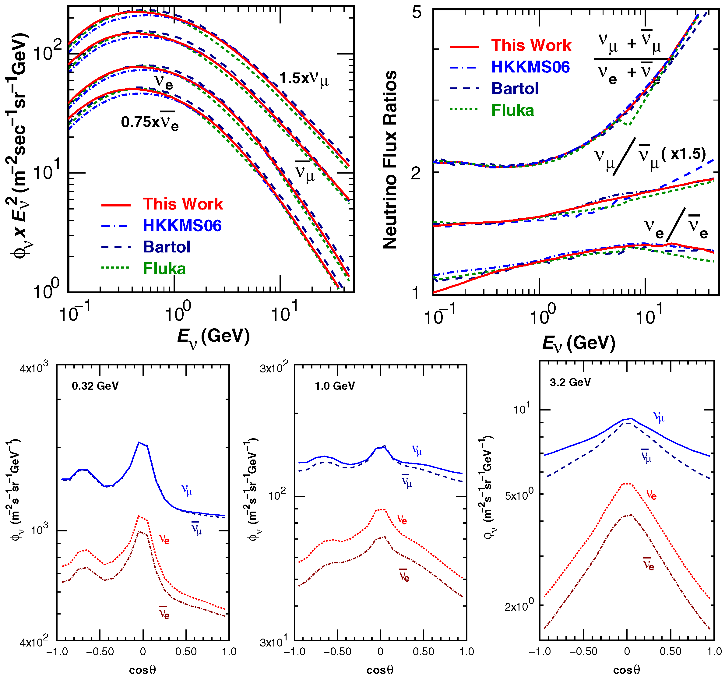
Atmospheric neutrinos are generated from the decay of and K, which are secondary particles resulting from the interaction of cosmic rays with air molecules in the Earth’s atmosphere. They come from all directions into detectors although their flux depends on the zenith and azimuth angles of the direction of their arrival. The flux in the horizontal direction is generally higher than that in the vertical direction, because of the longer path taken by parent particles through the atmosphere. The energy from atmospheric neutrinos exists in a wide range of 100 MeV to PeV scale measurements along a power-law spectrum, as shown in the Figure 1. The reason fewer neutrinos are produced at higher energies is mainly due to the falling primary cosmic-ray spectrum. The effect that the decay lengths are longer than the paths in atmosphere and the parent particles reach the ground before decaying, plays a role. It is also relevant for the energy dependence of and ratio and causes the neutrino flux to peak at the horizon as shown in the right Figure 1. The energy distribution is suppressed below the GeV energy region due to the rigidity cutoff effect of the primary cosmic rays by Earth’s magnetic field. The trajectories of charged particles in primary cosmic rays are affected by geomagnetic fields. Only particles that interact in the atmosphere before curving back into the space produce atmospheric neutrinos. The trajectory depends on the particles’ momentum and total charge; the ratio of them is called “rigidity”. Geomagnetic fields affect particles with lower energy more strongly; therefore, low-energy atmospheric neutrino flux is suppressed, a process that is called “cutoff”. Since Kamioka is located at a rather low geomagnetic latitude, it has a high local vertical rigidity cutoff. In addition, due to its strong azimuthal asymmetry, the cutoff is higher for particles arriving from the east than from the west. This east-west asymmetry arises from the fact that the primary cosmic rays are positively charged. On the other hand, in high-energy regions, above a few tens TeV, neutrinos from charm mesons’ decay are considered, instead of and K decay, due to the much shorter lifetimes of these charm mesons which are on the order of s. These are called “prompt” neutrinos [18,19], which are uniformly generated in the atmosphere, with equal fluxes of and .
Precise predictions of the atmospheric neutrino have been performed by several research groups, including HKKM [20], Bartol [21], and FLUKA group [22]. The differences among these models are choices of hadronic models and measurements of the primary cosmic-ray spectrum. Figure 1 shows a comparison of atmospheric neutrino fluxes and neutrino flux ratios calculated by different groups. The flux calculations differ by about 10%. Another feature is that the flavor ratio between and below the GeV scale is approximately two; however, it increases with the energy levels, as shown in Figure 1, because the muons produced by decay reach the ground before decaying. Time variation in the atmospheric neutrino flux is also expected. Long-term variation is due to solar activity with an average period of 11 years. The primary cosmic-ray flux at Earth is anticorrelated with the solar activity because the plasma from the Sun scatters the cosmic rays, and the cosmic-ray flux is reduced during periods of high solar activity. Consequently, the atmospheric neutrino flux is also predicted to be anticorrelated with solar activity. There is also yearly variation due to seasonal temperature variations that affect atmospheric density which increases in summer, when relatively more neutrinos are produced.
1.3. Neutrino Interaction
Interactions with nuclei in water (or ice) and rocks surrounding the detector are the norm in atmospheric neutrino observations, and that with electrons is negligible as the cross-section is three orders of magnitude smaller than that with nuclei. Interactions can be classified into charged-current (CC) or neutral-current (NC) interactions according to the type of bosons that are exchanged, or , respectively. A CC interaction produces a charged lepton, electron or muon, whose flavor corresponds to that of a neutrino, or . Therefore, the original neutrino flavor is identified by distinguishing the flavor of the related charged lepton. However, an NC interaction does not indicate the neutrino flavor since the outgoing lepton is a neutrino. The following neutrino interactions are dominant in the atmospheric neutrino energy region,
- Charged-Current quasi-elastic scattering: + N + N′
- Charged-Current pion production: + N + N′ +
- Deep Inelastic Scattering (DIS): + N + N′ + hadrons
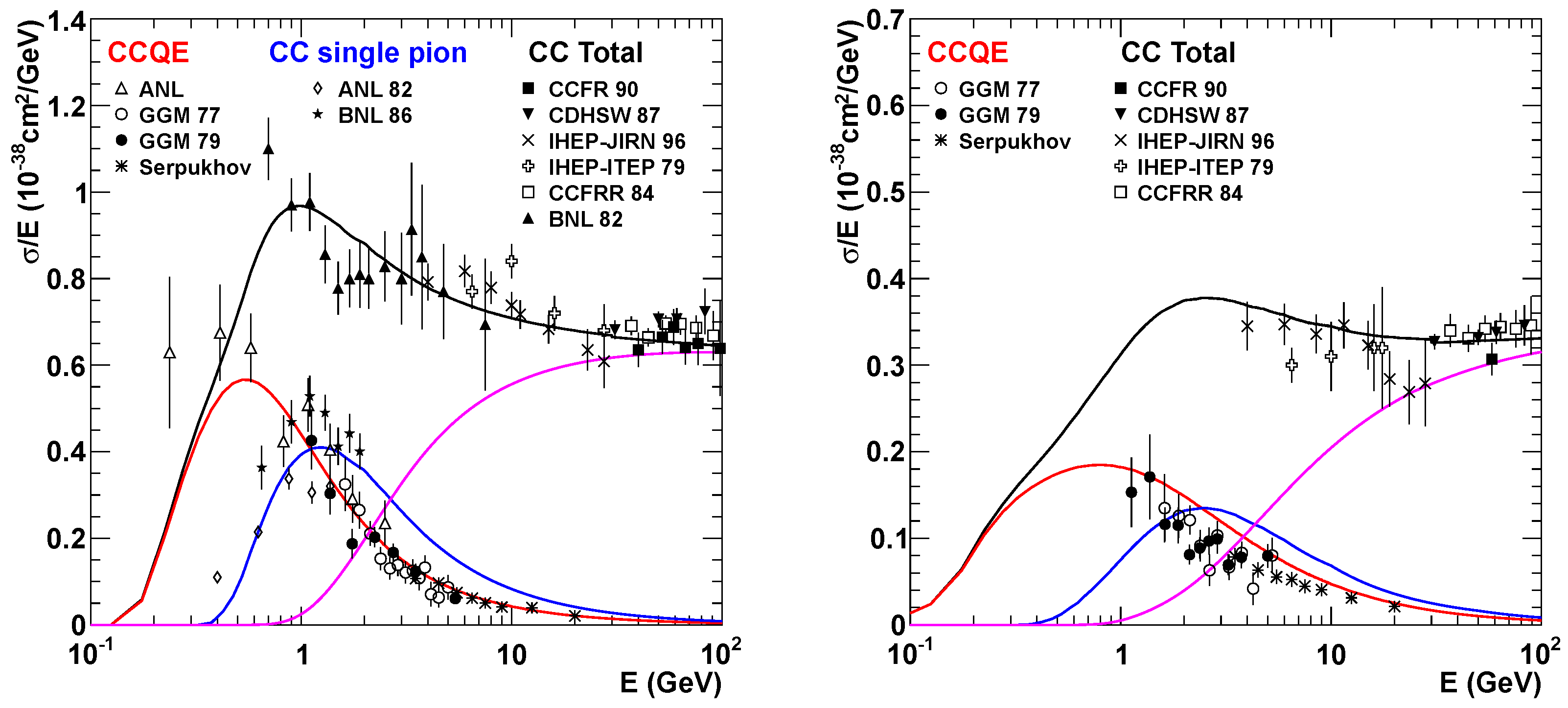
where N and N′ are nucleons (proton or neutron) and l is a charged lepton (CC) or neutrino (NC). Here, pion production is realized via resonance excitation. To generate neutrino interactions, there are several pieces of simulation software. Figure 2 shows the total cross-section of in total and each interactions predicted by NEUT [24] version 5.3.6, which was used in the latest atmospheric neutrino analysis in Super-Kamiokande. In this model, charged-current quasi-elastic interactions are simulated using the Llewellyn-Smith formalism [25] with nucleons distributed according to the Smith-Moniz relativistic Fermi gas [26] assuming an axial mass GeV/c and form factors from [27]. Interactions on correlated pairs of nucleons have been included following the model of Nieves [28]. Pion production processes are simulated using the Rein-Sehgal model [29] with Graczyk form factors [30]. The cross-section in this model are consistent with several experimental results.
1.4. Neutrino Oscillation
Neutrino oscillation occurs if flavor eigenstates are mixed with mass eigenstates, and a difference in mass exists. The mixing between flavor eigenstates () and mass eigenstates () can be written as
In the three-flavor neutrino framework, U is Pontecorvo-Maki-Nakagawa-Sakata (PMNS) mixing matrix [44,45,46], and usually parametrized by three mixing angles (), and one CP-violating Dirac phase () in neutrino oscillations as follows:
where and represent and , respectively. Neutrino oscillation frequencies are determined by the neutrino mass differences, and , where , , and are the three mass eigenvalues. Among these oscillation parameters, and have been measured by solar and reactor neutrino experiments, and have been measured by atmospheric and accelerator neutrino experiments, and has been determined by reactor neutrino experiments. The order of absolute mass ( in a normal ordering or in an inverted ordering) and the CP phase () are still unknown parameters. The dominant neutrino oscillation in atmospheric neutrinos is a channel between and caused by the parameters of the mass eigenstate between and . In addition, the appearance of oscillation from to is considered to be a sub-leading effect. The dominant neutrino oscillation probabilities in a vacuum for atmospheric neutrinos are expressed as follows:
where L is the flight length of neutrinos and E is the neutrino energy. When neutrinos traverse the Earth, their matter potential due to the difference in the forward-scattering amplitudes of and , which induces a matter dependent effect on of neutrino oscillations [47], must be taken into account. In this scenario, the oscillation value in Equation (7) can be rewritten by replacing and for constant matter density,
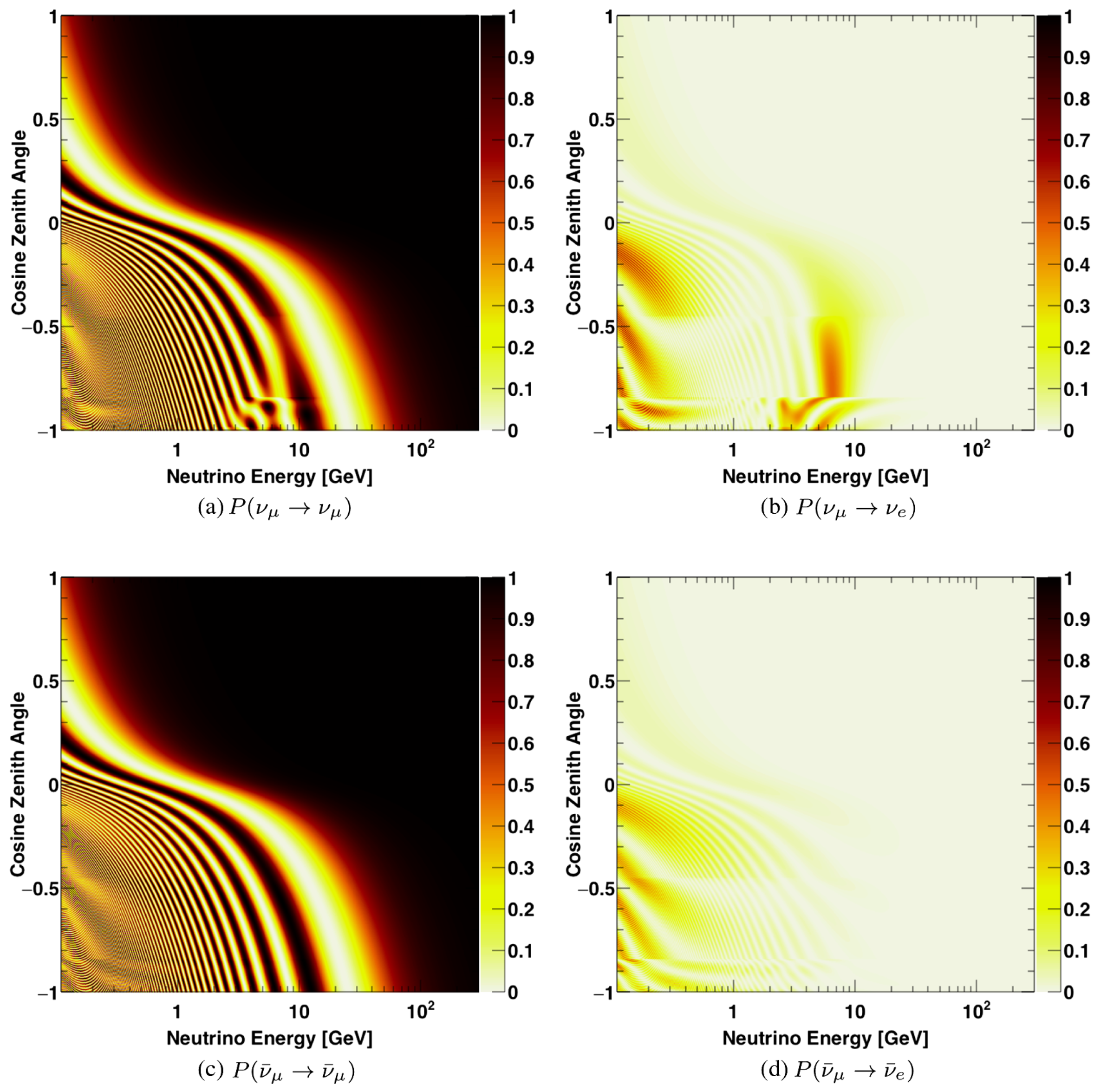
where is the effective matter potential, and the sign is positive for neutrinos or negative for anti-neutrinos; is the electron density, which is assumed to be constant; and denotes the Fermi constant. The potential is derived from the difference that which has both CC with electrons and NC with electrons and nucleons, while and have only NC. In this form, when , the effective mixing angle is resonantly enhanced. Since is positive, the enhancement only occurs for neutrinos if is positive which is as normal mass ordering, while it occurs for anti-neutrinos only in the case of the inverted mass ordering. Figure 3 shows the survival and transition probabilities for neutrinos and anti-neutrinos assuming a normal mass ordering. Earth matter effects suppress the disappearance of and enhance the appearance of especially in upward-going neutrinos, where the cosine zenith angle is negative, with energies in the range of 2–10 GeV. The appearance of in neutrino (b) in Figure 3 is enhanced in this energy region, while no clear enhancement appears in the anti-neutrino plot (d). If the mass ordering is inverted, this feature is switched and appears as an anti-neutrino case. Therefore, the difference in this level of enhancement between neutrinos and anti-neutrinos can help to determine the mass ordering in neutrino oscillation. The transition probability is also affected by the parameter, which results in a change of about 2% in the maximum total flux observed in the energy region less than 1 GeV.
2. Detectors
2.1. Super-Kamiokande
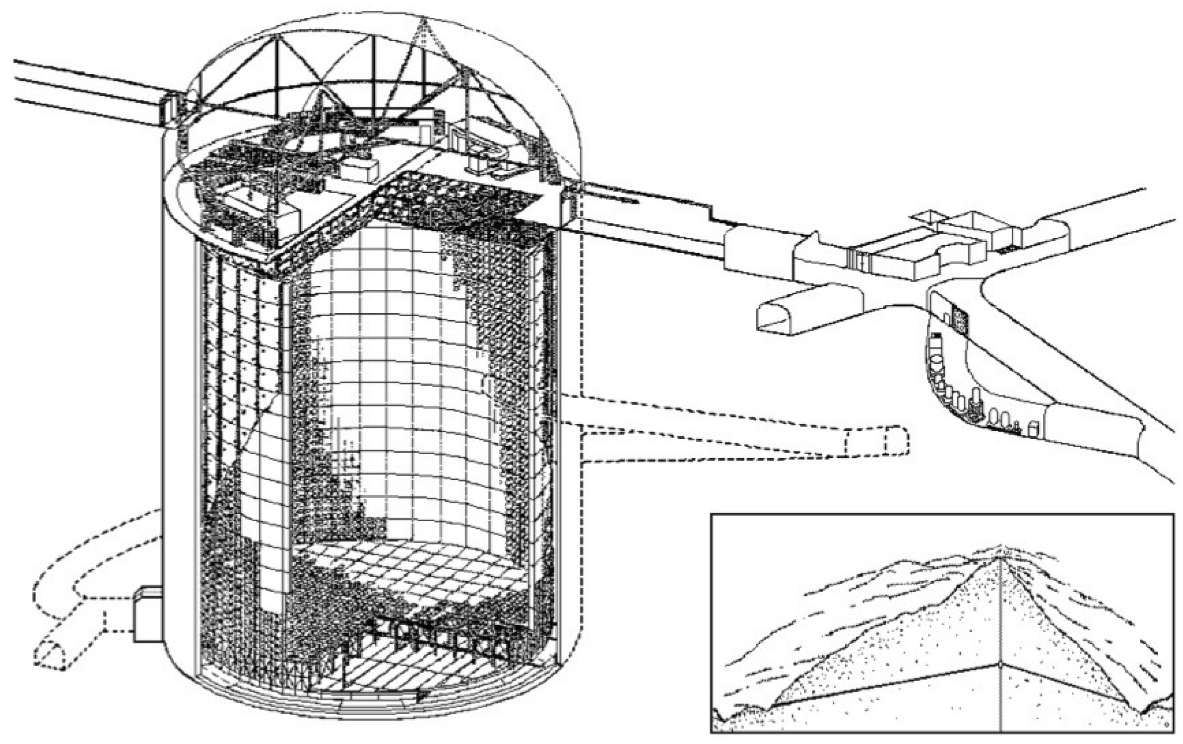
The Super-Kamiokande (SK) detector is a cylindrical tank of 39.3 m diameter and 41.4 m height, filled with 50 kilotons of pure water as shown in Figure 4. It is located 1000 m underground (2700 m water equivalent) in the Kamioka mine in Gifu Prefecture, Japan. The detector is divided into two regions called “inner” and “outer”, and lined with 11,129 twenty-inch PMTs in the inner detector and 1885 eight-inch PMTs in the outer detector. The signal detection method of SK is that Cherenkov light generated in water from the charged particles is observed by PMTs [49]. The fiducial volume used for the data analysis is 22.5 kilotons, which is within 2 m of the inner wall to maintain the detector performance. SK was launched in April 1996, and until now, there have been five experimental phases. The first phase lasted five years until July 2001. There were several successes in the detection of atmospheric neutrinos and solar neutrinos. However, a serious accident occurred in November 2001, in which most of the PMTs were broken. The experiment was resumed in October 2002, with about half the number of PMTs. Fortunately, even with half the number of PMTs, the atmospheric neutrino analysis was not affected greatly. After a three-year operation, full reconstruction was completed in 2006. The third phase, with almost the same number of PMTs as in the first phase, started in July 2006, and ended in August 2008. In the fourth phase, new electronics (QBEE [50]) were installed, which improved the detection efficiency of the decay electron from stopping muon higher. It is also possible to tag a 2.2 MeV gamma-ray, which is produced by the neutron capture by protons in water, even though it is about 20% detection efficiency. Neutron signals are useful for the improvement of atmospheric neutrino analysis. Although it is difficult to separate the neutrino and anti-neutrino events, information about the number of neutrons can be used to statistically differentiate between them because the number of neutrons in anti-neutrinos is larger than that in neutrinos. The fourth phase continued for 10 years until May 2018. SK was refurbished during the rest of 2018 to allow the loading of gadolinium to pure water. If gadolinium is loaded, the efficiency of neutron detection significantly improves by up to 90% depending on the gadolinium concentration. The main purpose of this gadolinium loading is the discovery of Diffuse Supernova Neutrino Background, but it also improves the analysis of atmospheric neutrinos due to the high neutron detection efficiency. After a successful refurbishment, the fifth phase started in January 2019.
In the atmospheric neutrinos observation in SK [51], the data sample is categorized by three distinct topologies: fully contained (FC), partially contained (PC), and upward-going muon (UPMU). FC events produce reconstructed interaction vertices inside the fiducial volume, while PC events also produce interaction vertices within the fiducial volume of the inner detector but are accompanied by considerable light in the outer detector. FC can be further sub-divided into single- and multi-ring and electron- and muon-like events. UPMU events are caused by muon-neutrino interactions in the surrounding rock, which produce penetrating muons. These muons either stop in the inner detector volume (stopping events) or continue through the inner detector (through-going events). The leptons, muons or electrons, generated by neutrino interactions preserve information from the original neutrinos, including the neutrinos’ flavor, energy, and direction. To identify muons or electrons, the Cherenkov ring pattern is used. An electron produces diffused ring patterns because of the electromagnetic shower and multiple scattering, while a muon produces a ring with a sharp edge. The SK atmospheric neutrino analysis uses event categories, reconstructed energy and direction, and particle types (muon-like or electron-like).
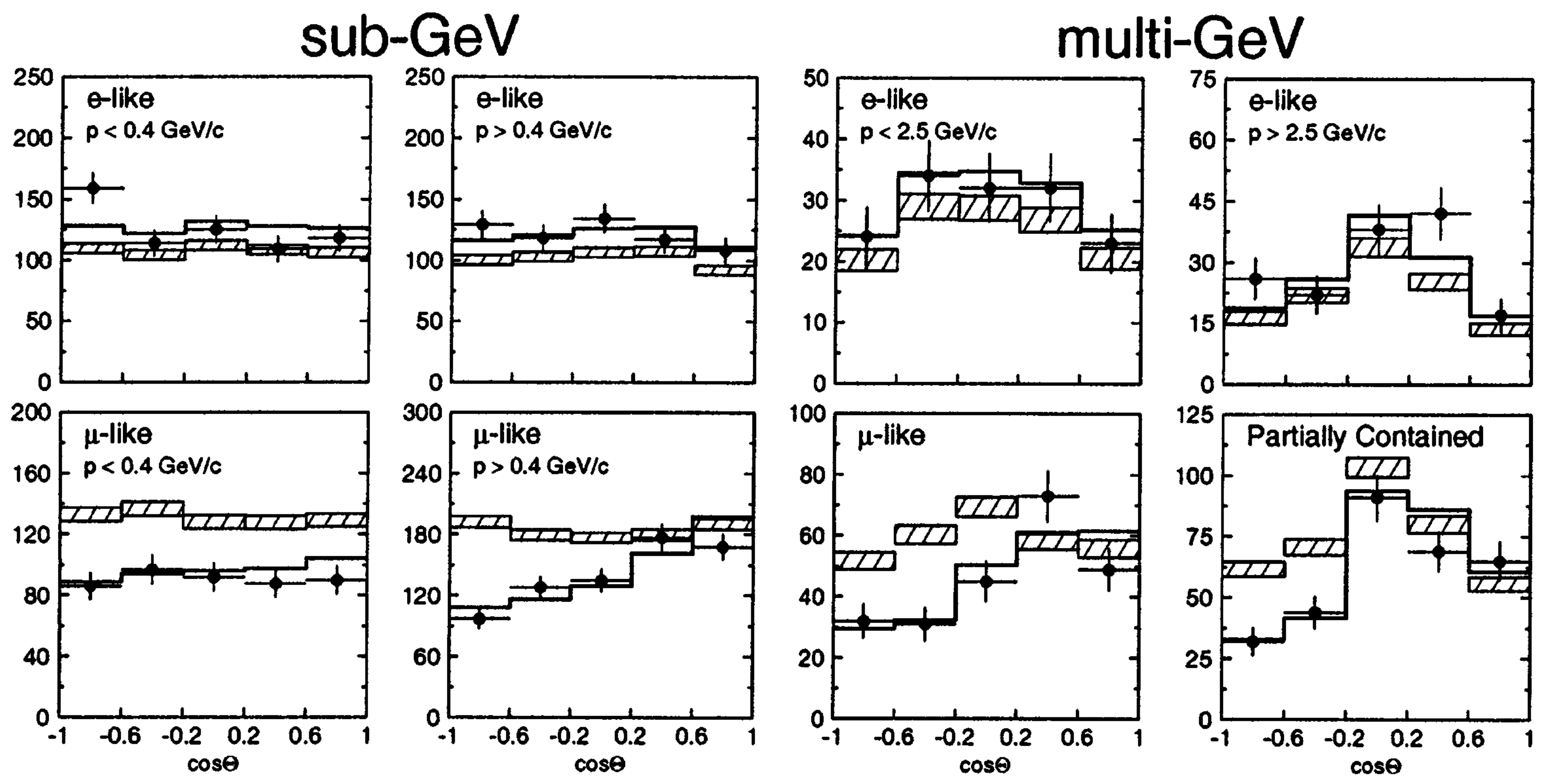
Discovery of the Neutrino Oscillation
Figure 5 shows several plots of zenith angle dependence on the first results obtained from SK in 1998 [15]. The electron-like events were consistent with the predicted results, while the number of upward-going muon-like events were significantly smaller than that of the downward-going events. This was evidence of the neutrino oscillation that muon-neutrinos converted to other flavor of neutrinos through the flight inside the Earth.
2.2. IceCube
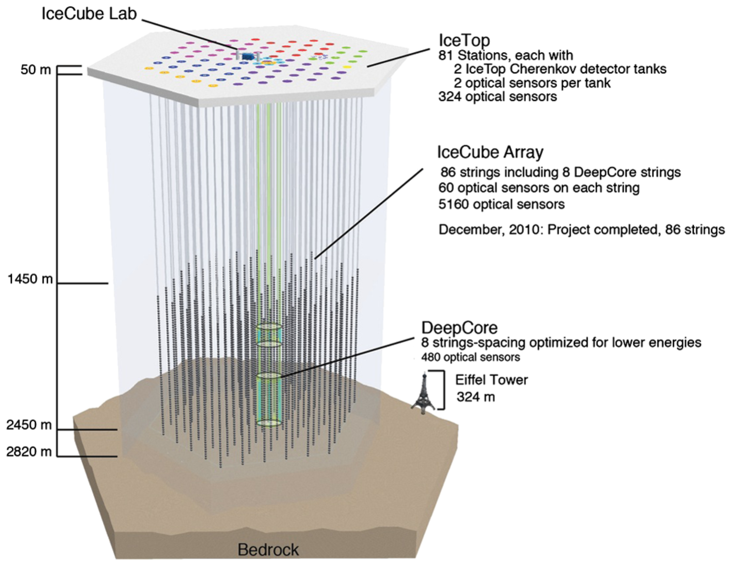
The IceCube is a cubic-kilometer neutrino detector buried in the Antarctic ice, as shown in Figure 6. It comprises 5160 digital optical modules (DOMs) along 86 vertical strings, with 60 DOMs per string. Each DOM houses a downward-facing 10-in PMT with electronics in a glass pressure sphere. Of the 86 strings, 78 are deployed with an inter-string distance of ∼125 m and a space of ∼17 m between each DOM at depths between 1450 and 2450 m below the surface. This part of the detector is optimized for the neutrino energy range of 100 GeV to 100 PeV. The remaining eight strings, located at the bottom center of the detector, are set more densely with DOMs. This detector, called DeepCore, comprises 647 DOMs with high-quantum-efficiency PMTs placed 2100 m under the clearest ice. DeepCore has a volume of m, and is optimized for the detection of lower-energy neutrinos down to 5.6 GeV.
IceCube observes Cherenkov light generated in ice by charged particles resulting from neutrino interactions. As the target neutrino energy for IceCube is high, deep inelastic scattering is a dominant feature in neutrino interaction. The observed events are categorized into two types of patterns: long, straight tracks produced by muons (track-like) and spherical cascades produced by electromagnetic and/or hadronic showers (cascade-like).
IceCube observation was fully commissioned in 2011. One important result was the discovery of two ultrahigh-energy (∼PeV) neutrinos in 2013 [52]. Compared to the expected number of atmospheric neutrinos, , these two events were possibly of astrophysical origin.
2.3. ANTARES
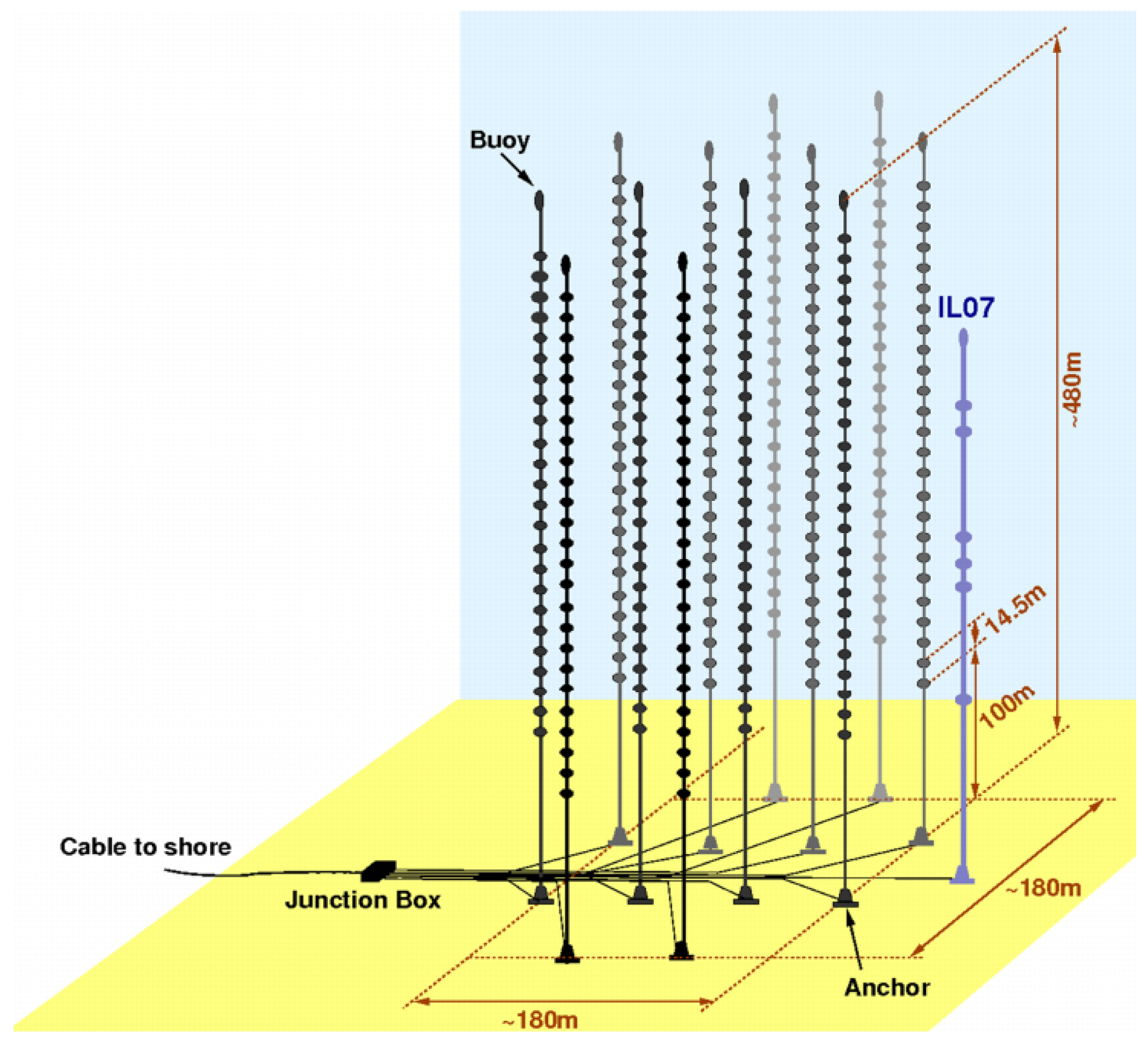
The ANTARES neutrino telescope is in the Mediterranean Sea at a depth of 2475 m [54]. A schematic view of the detector is shown in Figure 7. It comprises 12 detection lines: 11 equipped with 25 storeys of three optical modules and one line with 20 storeys of optical modules, giving a total of 885 optical modules. Each optical module has a 10-in PMT, whose axis points 45° downward. The detector was completed in 2008, and a total of 2830 days of data had been analyzed for atmospheric neutrino data by 2016.
2.4. Detector Summary
Table 1 shows the summary of three detectors for atmospheric neutrino research.
3. Oscillation Analysis of Atmospheric Neutrinos
3.1. Oscillation Parameter Determination
3.1.1. Super-Kamiokande
The main contribution to the understanding of neutrino oscillation from atmospheric neutrinos is the determination of and . Recently, all sub-leading effects of neutrino oscillation can be investigated due to precise observation and large statistics of data. Here, the earth matter effect plays an important role in neutrino oscillation schemes, which resolves mass ordering, two possible regions, and . It has different behavior of appearance between and for the mass ordering. However, SK is insensitive to the charge sign of particles; therefore, CC neutrino and anti-neutrino interactions cannot be distinguished on an event-by-event basis. Instead, they are statistically separated based on the number of decay electrons, number of Cherenkov rings, and transverse momentum. In the most sensitive energy region between 2 and 10 GeV, not only CC quasi-elastic interactions but also single pion production via resonance excitation and the deep inelastic scattering process should be considered. In single pion production, generated in an anti-neutrino reaction, such as , will be captured on an O nucleus, leaving the positron as the only detected particle and no delayed electron signal. In neutrino reactions, on the other hand, is generated via . It is not captured in this manner and produces a delayed electron signal through its decay chain. Thus, an anti-neutrino tends to produce a single-ring event without any delayed electron, while a neutrino event has the opposite effect. Due to the V-A structure of the weak interaction, the angular distribution of the leading lepton from is more forward than those from reaction, which means that the transverse momentum in is expected to be smaller than that in . The statistical separation of and is performed by a likelihood method using the above variables.
For a constraint on the neutrino oscillation parameter, the data obtained in SK are fitted to expectations by MC simulation using a binned method. There are 520 analysis bins in total (energy and zenith angles in each event category) for each SK phase and 155 systematic uncertainties. Figure 8 shows the chi-square differences from the minimum as a function of (or ), and , for the normal and inverted mass ordering cases using 5326 days of data from SK measurements [48]. From the results, the normal mass ordering showed better agreement than the inverted mass ordering with . The best-fit neutrino oscillation parameters in the normal mass ordering were radians. In addition, a neutrino oscillation analysis with constraints from other experiments was provided. One concerned reactor short-baseline neutrino experiments, Daya Bay, RENO, and Double Chooz, for , and the central value of these experiments was [55]. The other concerned Tokai-to-Kamioka (T2K) long-baseline neutrino experiment [56]. Since SK is the far detector of T2K, many experimental aspects, for example, the detector simulation, the neutrino interaction generator (NEUT), and the event reconstruction tools, are common between them. Thus, it is possible add published binned T2K data to the SK atmospheric neutrino fit for determination of the neutrino oscillation parameters. When the constraints on from the reactor experiments were applied to atmospheric neutrinos, the preference for the normal mass ordering was . When the T2K constraints were added, it became stronger at .
3.1.2. IceCube
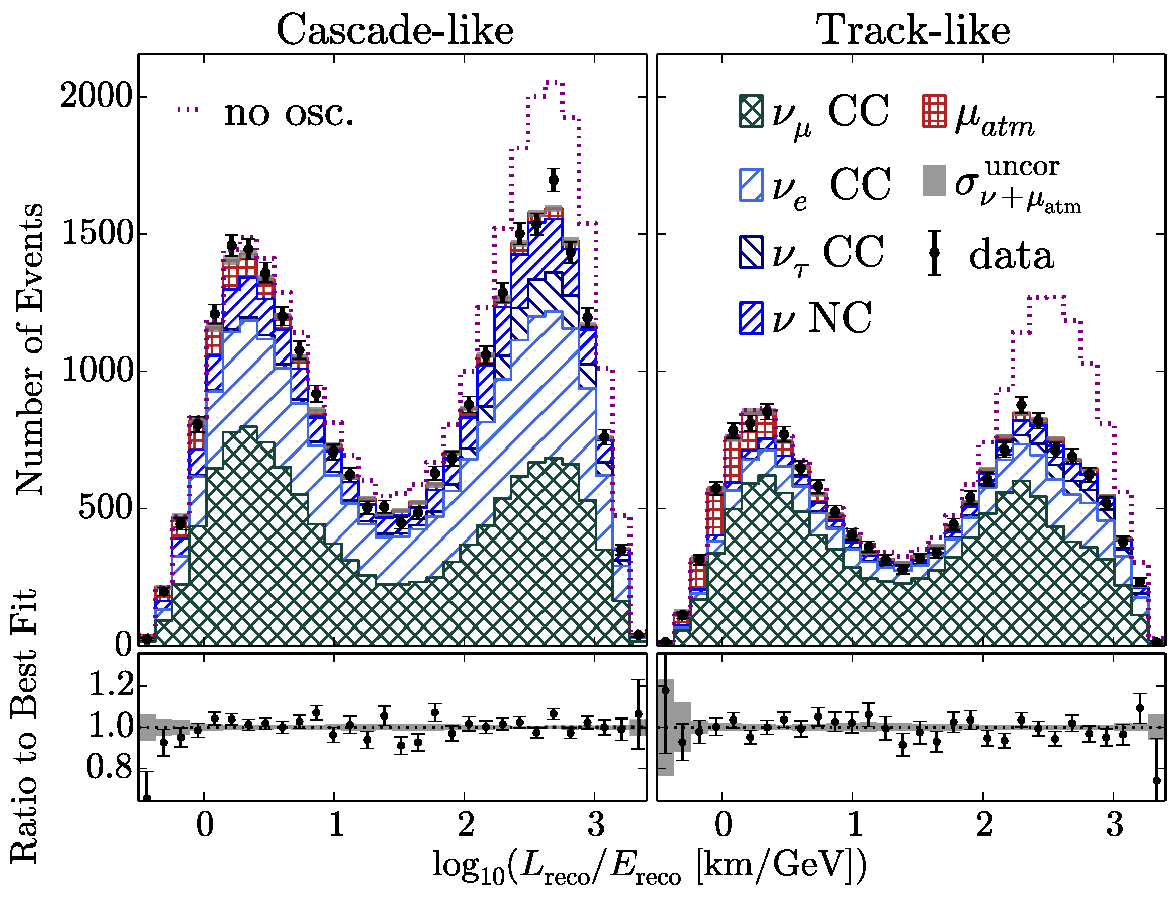
Measurements of the atmospheric neutrino oscillation parameters of and in IceCube were reported in 2018 [57]. The unique characteristics of IceCube detector for the atmospheric neutrino search are, at first, the high statistics due to the huge volume. It is also possible to detect downward-going muon events induced by atmospheric neutrino interaction using the surrounding IceCube detector to distinguish with cosmic-ray muons. To provide a constraint for the neutrino oscillation parameters, the reconstructed neutrino energy (8 bins) and zenith angle (8 bins), both track-like and cascade-like, were fit to the expectations using a binned method. Here, the reconstruction was performed by calculating the likelihood of the observation of photoelectrons by DOMs as a function of the neutrino interaction position, direction and energy. The best-fit neutrino oscillation parameters were assuming a normal mass ordering. Figure 9 shows the distribution along with the corresponding predicted counts given the best-fit neutrino oscillation parameters broken down by event type for both track-like and cascade-like events. The two peaks corresponded to down-going and up-going neutrino trajectories. As the track-like sample was enriched in CC events, up-going events were strongly suppressed in track-like events due to neutrino oscillation. While the cascade-like sample was evenly divided between CC events and interactions without a muon in the final state, some suppression could also be observed.
3.1.3. ANTARES
The measurement of the atmospheric neutrino oscillation parameters of and in ANTARES was reported in 2019 [58]. The energy for the atmospheric neutrino analysis in ANTARES ranged from a few tens of GeV up to 100 GeV. Track-like events originating from the penetrating muons produced via CC interactions of were used for the analysis. On the other hand, shower-produced events, for example, electromagnetic showers from CC interactions or hadronic showers from NC interactions, were regarded as the background events. Here, muon-track reconstruction was essential, and two different algorithms were used: one in which PMT hits were selected to find the best muon track and another involving fitting to a chain at each step to improve the track estimation. Once the muon track was reconstructed, the muon energy was estimated from its track length, given a constant energy loss of muons in the sea at 0.24 GeV/m in the energy range of 10–100 GeV.
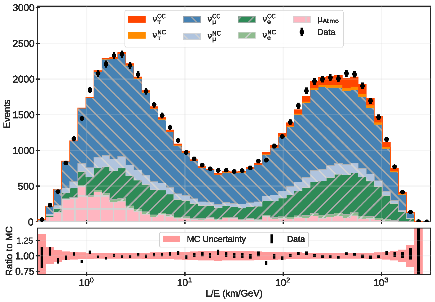
To obtain a constraint for the neutrino oscillation parameters, a logarithmic base-10 scale of reconstructed neutrino energy in GeV was divided into eight bins, seven from 1.2 to 2.0 plus an additional underflow bin for . The cosine zenith angle was divided into 17 bins from 0.15 to 1.0. The fit was performed using a log-likelihood approach. The best-fit neutrino oscillation parameters were degree. Figure 10 shows the reconstructed energy divided by the cosine of the reconstructed zenith angle. The lowest bin of this plot is expected to be affected by neutrino oscillation. The data showed good agreement with neutrino oscillation assumptions.
3.1.4. Constraints on and
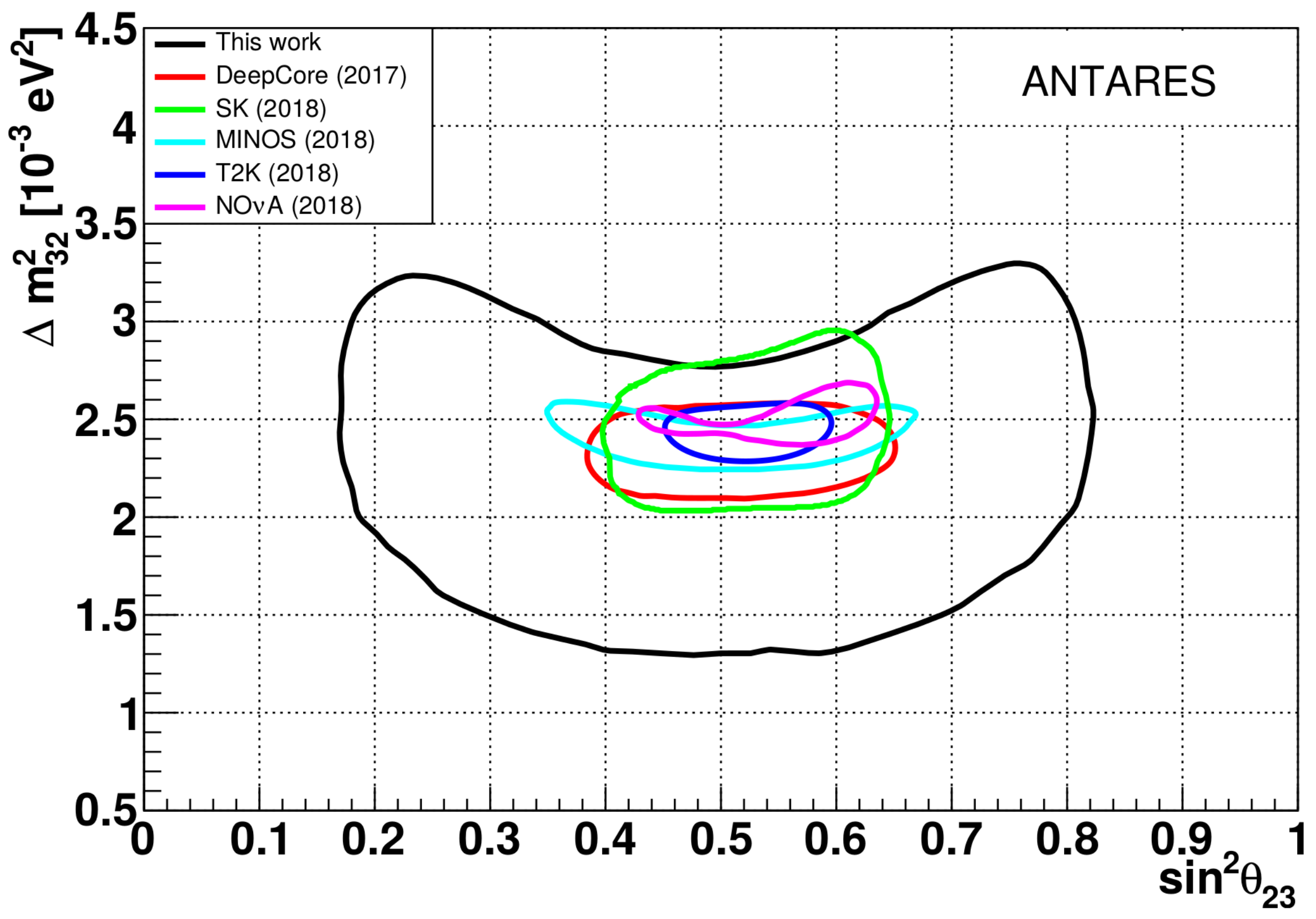
Figure 11 shows the allowed region of neutrino oscillation parameters ( and ) at 90% C.L. overlaying several experiments both for atmospheric and accelerator neutrinos. Even though there are different sources of neutrinos, and the sensitive energy range is different in atmospheric neutrino experiments, all results showed good agreement with each other.
Here, the MINOS far detector, which is 5.4 kTon mass of iron-scintillator tracking calorimeter, is used for the study of atmospheric neutrinos as well as neutrinos originating from the Fermilab NuMI accelerator beam. The far detector is located at underground (2070 m water equivalent) in Soudan mine, Minnesota, USA. The detector is magnetized and it enables the separation of and on an event-by-event basis using the curvature of the produced charged muon. The contour of MINOS in the figure was combined results of accelerator neutrinos and 60.75 kt-year data of atmospheric neutrinos.
3.2. Tau-Neutrino Appearance
The dominant channel of the atmospheric neutrino oscillation is transition between and in the standard scenario. Actually, the long-baseline neutrino beam experiment from CERN to GranSasso, OPERA, which is sensitive to the same neutrino oscillation parameters as atmospheric neutrinos, found the appearance from to neutrino oscillation [62]. Finally, OPERA observed 10 events with a background expectation of , which was equivalent to 6.1 level of discovery significance. The appearance should also be seen in the atmospheric neutrino data.
3.2.1. Super-Kamiokande
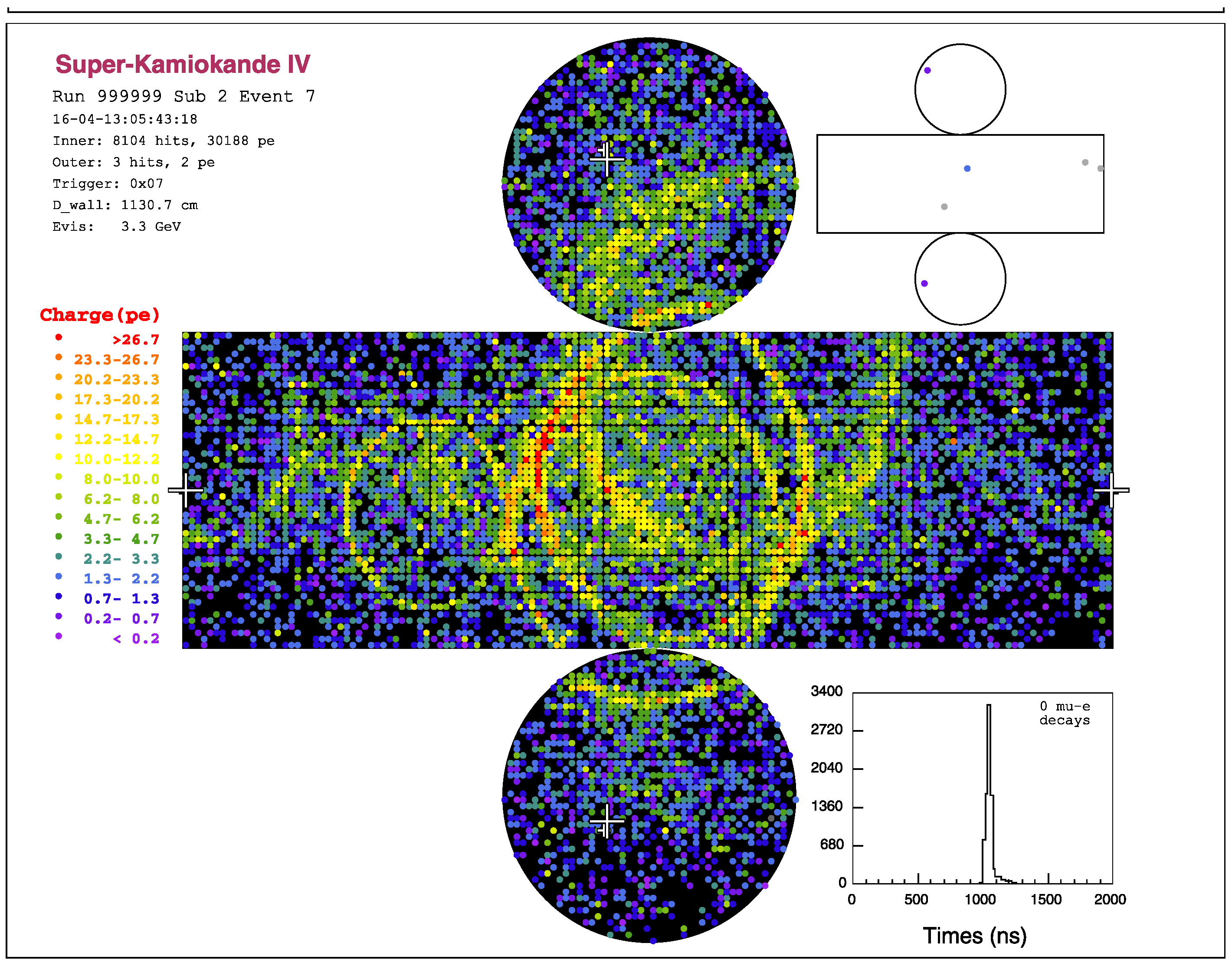
In the atmospheric neutrino observation by the SK detector, the deficit of upward-going events due to the neutrino oscillation passing through the Earth was observed. The original is considered to change to . The appearance of was also searched by SK [63], but the detection was challenging. Since the atmospheric neutrino flux falls as and charged-current interactions only occur above the lepton production threshold, 3.5 GeV, the expected rate at SK is only one event per kiloton per year. Furthermore, events are difficult to identify individually as they tend to produce multiple visible particles in the SK detector, as shown in Figure 12.
An analysis was performed that employed a neural network technique to discriminate between “tau-like” and “non-tau-like” events from the hadronic decays of detected by SK from atmospheric and background events. The following seven variables were used as inputs to the neutral network: (1) total visible energy: signal events are expected to have higher visible energy compared to the background events; (2) shower-like events: hadronic decay of events tend to make a shower in the ring pattern; (3) number of decay electron candidates: pions produced by the hadronic decay of produce more decay electrons than the background events; (4) distance between the primary interaction point and decay electron vertex: pions are expected to have smaller momentum compared to the background; (5) sphericity, which is the evaluation whether isotropic or not: hadronic decay of is more isotropic than the background; (6) number of Cherenkov ring fragments: events are expected to have more ring candidate; (7) ratio of the observed photons and the most-energetic ring in an event: events are expected to be small because energy is carried by multiple particles in the hadronic decay of . When “tau-like” events are selected from neural network output in this analysis, 76% of signal events and only 28% of background events remain which is estimated by the simulation.
To evaluate whether a signal was being observed, the maximum likelihood method was used. The output of a neural network and reconstructed zenith angles were used to construct the probability density function (PDF) for both signals and the background using simulation. As is generated via neutrino oscillation through the Earth, signals tend to be an upward-going event, which is why the zenith angle was used for the PDF. In this analysis, the 5326 days of atmospheric neutrino data in SK was fitted to the following function:
where is a normalization factor of tau signal, is a i-th systematic error. According to the normalization factor , the failure of tau to appear is zero and the appearance of a tau signal is one. It was found to be , assuming the normal mass ordering of neutrino mass splitting, which is equivalent to a 4.6 level of appearance. Assuming an inverted mass ordering, it was , and the significance was . Figure 13 shows the zenith angle distribution for both tau- and non-tau-like events, along with the expectation fitted to tau and the background. These plots show good agreement between the data and MC simulations.
Based on the significant discovery of the event, the charged-current tau-neutrino cross-section was also calculated. The measured cross-section was expressed as , where is the flux-averaged theoretical cross-section. It was calculated by the integral of the differential charged-current cross-section weighted with the energy spectrum of atmospheric from neutrino oscillations, and was found to be cm. Finally, the measured cross-section integrated from 3.5 to 70 GeV was calculated as cm.
3.2.2. IceCube
A search for appearance by neutrino oscillation using atmospheric neutrino samples by IceCube/DeepCore was performed [64]. The energy region ranges from 5.6 to 56 GeV, which was the same as that in the neutrino oscillation analysis. The identification of individual events by DeepCore is difficult because of the tau lepton produced via CC interaction decays with a small track length of ∼1 mm, compared to the position resolution of the detector. To search for the appearance of by neutrino oscillation, the distortion of neutrino energy and direction in cascade-like events compared to non-neutrino oscillation assumption were investigated. In the data analysis, two independent methods were applied: one targeted a high acceptance of all neutrino events, whose background estimation was simulation-driven, and the other was optimized for a higher rejection of non-neutrino events, with data-driven background estimation. Both methods used a boosted decision tree for event selection and background rejection. The neutrino energy and direction were reconstructed by the maximum likelihood method using the charge and time observed by DOMs.
Figure 14 shows the distribution along with the corresponding predicted counts, given the best-fit neutrino and cosmic-ray muon broken down for the first method of analysis. The plot showed good agreement between the data and the model. The normalization factor of appearance in DeepCore was found to be which is equivalent to a 3.2 level of appearance. The result was consistent with those obtained for SK measurements.
3.3. Sterile Neutrino Analysis
The existence of neutrino oscillation has been established by a wide range of experiments using different sources of neutrinos: the atmosphere, the Sun, nuclear reactors, and accelerators. However, not all neutrino experiments show the three standard flavors of neutrinos. For example, an excess of electron neutrinos in a muon-neutrino beam with eV was found in the LSND [65] and MineBooNE [66] experiments. Additional anomalies appeared in the and rates in several reactor experiments [67] and gallium-based experiments [68]. These results made a hint of neutrino oscillations driven by a eV. On the other hand, the number of neutrinos was measured as light neutrino flavors by large electron-positron(LEP) collider using the width of the Z mass peak [69]. This result required that its mass of an additional neutrino is either heavier than half the Z boson; however, it is difficult to be a player of neutrino oscillations, or not interact via weak interactions, which is called sterile neutrinos.
To introduce N additional sterile neutrinos, U in Equation (1) should be matrix. The matter effect in neutrino oscillation for sterile neutrinos should also be considered. Since sterile neutrinos have no CC nor NC interactions, the effective matter potential is expressed by . It is derived from the difference from and which have only NC. Here, NC depend only on neutron density () because the interactions with electrons and protons are equal and opposite, and their densities are identical in neutral matter.
Atmospheric neutrino samples can also make a constraint on sterile neutrinos due to a wide range in both energy and travel distance. The results of single additional sterile neutrino scenario, called the “3+1” model, have been reported by SK [70], IceCube [71], and ANTARES [58]. Actually, it hard for this model to explain all the anomalies consistently; however, it can be extended to models with more than one sterile neutrino although it needs more parameters. The “3+1” model, denoted as U, is that a neutrino flavor eigenstate with mass eigenstate should be added in the mixing matrix defined in Equation (2). In this model, six new parameters are added: three mixing angles , two CP-violating phases, and one mass differences To search for sterile neutrinos using atmospheric neutrinos, several assumptions were made. First, since the assumed mass difference between the mass eigenstate and the other is large, is averaged as 1/2. Second, the other parameters, except for , ( only for ANTARES), are ignored since they have negligible impact on atmospheric neutrino oscillation. The effect of these neutrino oscillation parameters results in a different disappearance pattern compared to the standard neutrino oscillation scheme.
The analysis method is similar to the standard three-neutrino hypothesis, i.e., fitting the reconstructed energy and cosine zenith angle from the experimental atmospheric neutrino data to the prediction but using only the disappearance channel. No clear evidence of sterile neutrinos was found in these experiments. Figure 15 shows the exclusion region at 90% and 99% C.L. in the and parameters.
4. Atmospheric Neutrino Flux Measurements
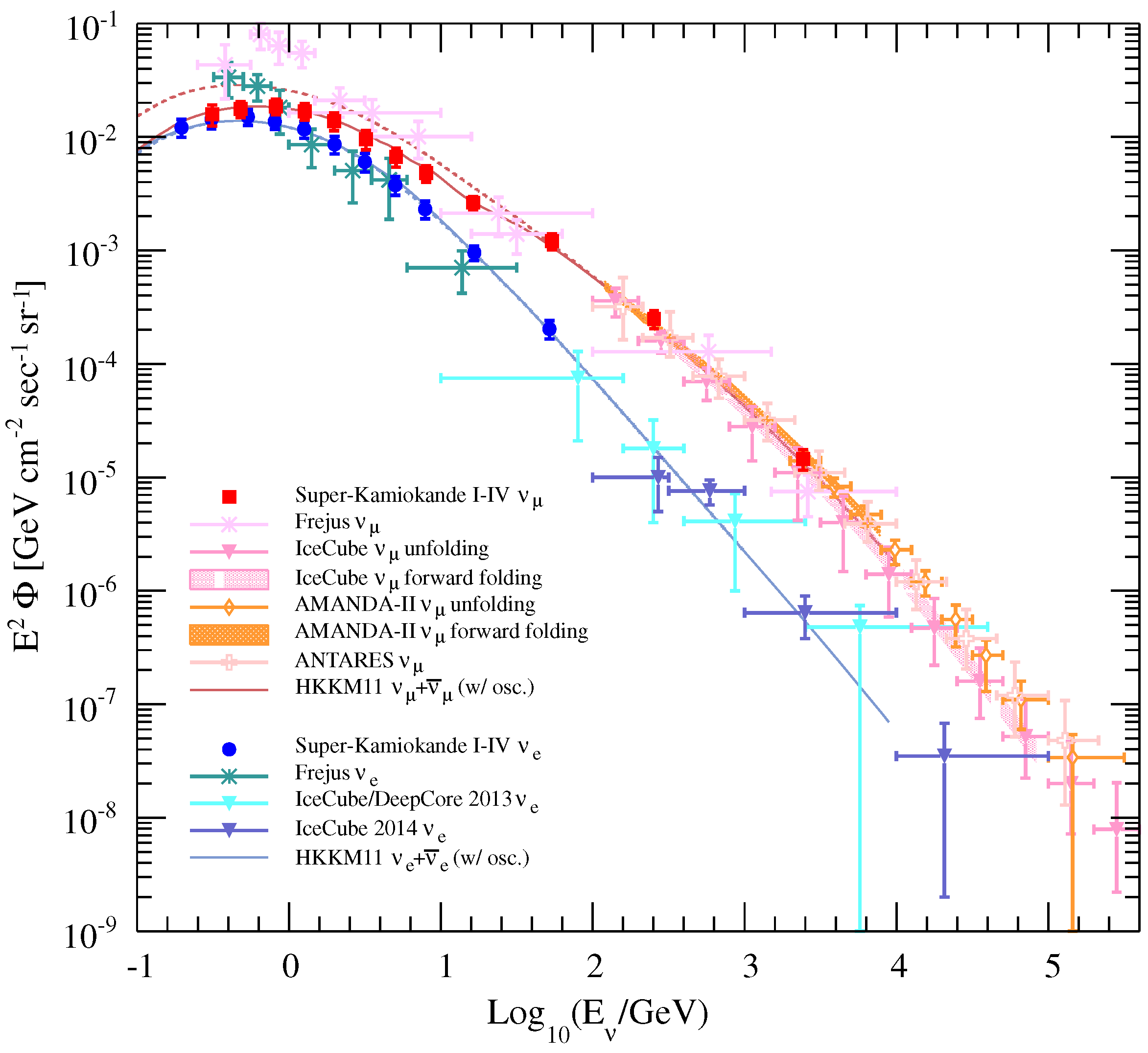
Predictions and observations of the atmospheric neutrino flux have been reported by several groups. Its energy distribution is derived from charged particles, mainly muons or electrons, induced by neutrino interaction. Figure 16 shows several predictions and measurements of the energy distribution in atmospheric neutrinos. In this figure, SK applies the so-called “unfolding” method to all experimental phases [72]. The event rate of the observed charged particles induced by atmospheric neutrinos is expressed as the convolution of neutrino flux, neutrino oscillation probability, neutrino cross-section, and detector efficiency. The obtained atmospheric neutrino spectrum is derived from the deconvolution of the above observed values, which is the unfolding method. The observed flux of atmospheric and is indicated by the red square and blue circle in Figure 16, and are consistent with the predictions that include an assumption of neutrino oscillation. The values (p-value), including and together, are 22.2 (0.51) for HKKM, 30.7 (0.13) for Bartol, and 25.6 (0.32) for FLUKA, with a degree of freedom of 23.
IceCube reported the results of atmospheric and flux. In the analysis, the observable value is the deposit energy per track length of muons in the detector (). It is a convolution of the atmospheric neutrino flux and the response matrix, which accounts for the effect of propagation through the Earth, neutrino interaction, detector response, and event selection. Unfolding of the atmospheric muon-neutrino flux from 100 GeV to 400 TeV was performed [73], and the results are indicated by the pink triangle in Figure 16. In addition, the so-called forward-folding analysis was applied, in which the distribution was tested against the hypotheses of muons arising from atmospheric by or K decay, prompt , and astrophysical [53]. At first, no evidence was found for an astrophysical or prompt . In a comparison with HKKM, the normalization factor of the absolute atmospheric neutrino flux was found to be and the spectra index was found to be steeper by . The allowed regions of these parameters from 332 GeV to 84 TeV are indicated by the pink band in Figure 16. As for the atmospheric measurements by IceCube, two results were reported: one was a low-energy region (80 GeV to 6 TeV) using DeepCore [74] and the other was a high-energy region (0.1 to 100 TeV) using the full IceCube detector [75]. After several steps of background reduction, related to in the main sample and cosmic-ray muons from the cascade sample, the data were fitted to the prediction to obtain the atmospheric flux. The observed flux was consistent with the prediction, as shown in Figure 16. In addition, no prompt neutrino signal was found for .
ANTARES reported the atmospheric energy spectrum in the energy range between 0.1 and 200 TeV [76]. It was derived from the measured muon energy distribution through a response matrix, determined from simulations, and an unfolding method. The results are shown in the figure, although it is admittedly busy. The overall normalization factor is 25% higher than the prediction in [21], and the flux is compatible with the IceCube results. The prompt neutrino was not observed in the ANTARES data.
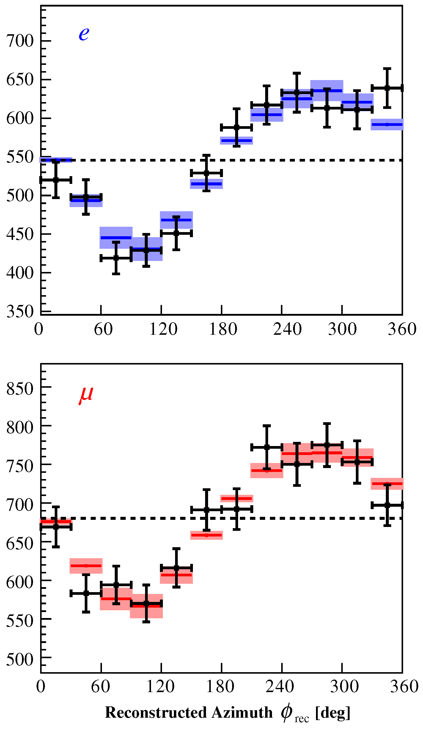
An east-west flux asymmetry of atmospheric neutrinos due to the rigidity cutoff is predicted. SK reported the measurement of this effect [72] using an FC sample, selecting both electron- and muon-like events with a single reconstructed Cherenkov ring. Figure 17 shows the azimuthal distribution of the subsample event selected to optimize the significance of the east-west dipole asymmetry. The effect is observed at a significance level of 6.0 (8.0) sigma for the muon-like (electron-like) samples. The dependence of the asymmetry on the zenith angle was also investigated and was observed at the 2.2 sigma level. These effects were consistent with the prediction within the given uncertainties.
SK also reported long-term and seasonal atmospheric neutrino flux variations [72]. An anti-correlation with solar activity was predicted for the long-term variation and a weak preference for a correlation was observed at the 1.1 sigma level using 20 years’ observation. The seasonal variation is considered to be occurred by the change in the atmospheric density profile over the year; however, no such correlation was observed in SK.
5. Future Prospects
In this section, the search for atmospheric neutrinos by next-generation neutrino detectors is briefly described. Table 2 shows the summary of the detectors. Succession to the current water Cherenkov detector experiments are now proposed. Here, an enlargement of the volume in underground detector and denser photo-sensor in string type detector are crucial to determine unknown neutrino oscillation parameters such as mass ordering and CP-violating phase.
Hyper-Kamiokande (HK) [77] is underground (1750 m water equivalent) water Cherenkov detector, located 8 km from the SK site. It is based on the well-established technology with a fiducial volume of 187 kilotons, which is 8.3 times larger than that obtained for SK, and will start operation in 2027. It consists of 40,000 high-quantum-efficiency PMTs for inner detector. The second HK detectors in future is also proposed [78].
The IceCube plans detector upgrade as “IceCube-Gen2” [79]. The first step of the upgrade is scheduled for deployment in the 2022/2023 polar season [80]. It is proposed that 7 additional strings with 125 optical modules spaced 2.4 m apart, which is denser than IceCube/DeepCore, will set in a small part of IceCube observatory (2 MegaTon of ice). A denser detector, PINGU [81], that consists of 26 strings with 192 optical modules spaced 1.5 m apart, is proposed as a goal of IceCube-Gen2. The denser photo-sensor enables the neutrino oscillation parameter determination with high precision [82].
The successor of the ANTARES is KM3NeT [83]; it is a deep-sea neutrino detector in the Mediterranean Sea. There are two installation sites for different purpose; one is “ARCA” at 3500 m depth in Italy which aims an observation of high-energy neutrino sources in the Universe, the other is “ORCA” at 2500 m depth in France which aims a neutrino oscillation parameter determination using atmospheric neutrinos. The multi-PMT is set in the DOM as an optical sensor, and 18 DOMs (spaced 9 m apart for ORCA) are hosted in one string that is called “Detection Units (DU)” The detector construction was started, and its performance has been checked [84]. The first DU for ORCA had already been installed, and 5 additional DUs will be installed soon, and finally 115 DUs will be installed.
Apart from water Cherenkov technique, several different types of detector available for atmospheric neutrinos are proposed. DUNE [85] is a long-baseline neutrino experiment using a massive liquid argon time-projection chamber (LAr TPC). The far detector is located at a depth of 4300 m water equivalent at the Sanford Underground Research Facility, in Lead, South Dakota, USA. One of the advantages of LAr TPC is excellent particle identification and better angular and energy resolutions than water Cherenkov detectors. The well reconstructed momentum of each final state particles enables the determination of the energy and direction of the incident neutrinos. The fiducial volume of one LAr TPC module is 10 kilotons. The first module construction has started, and 4 modules are the goal. The DUNE operation together with the neutrino beam will start in 2026; however, the atmospheric neutrino observation will be possible to start as soon as the first module completes when it is expected before 2026.
Main topics of the atmospheric neutrino observation in neutrino oscillations is determination of mass ordering. Any future detectors described here will reach more than 3 level to reject the incorrect mass ordering, assuming that either the normal or inverted mass ordering is true, after 5–10 years of operation, although this depends on other parameters of the neutrino oscillation. The precise tau appearance observation and studies of any exotic model are also possible.
6. Summary
The research into atmospheric neutrinos has had great success in the last two decades, notably the discovery of neutrino oscillation by the SK detector. This paper reviews the recent achievements made in atmospheric neutrino observations by SK, IceCube, and ANTARES. First, the standard three-neutrino oscillation scheme, expressed by the PMNS matrix, was established and the parameters were determined. The appearance of tau neutrinos in atmospheric neutrinos, predicted by this theory, was confirmed. An exotic scenario, such as the appearance of sterile neutrinos, was tested; however, no clear signal was observed. The observed atmospheric neutrino flux was consistent with the predictions. Among the unknown neutrino oscillation parameters, the normal mass ordering is preferred in the current measurements; however, it is not significantly determined. Atmospheric neutrino observations in the next generation of neutrino detectors are expected to provide final determination of the mass ordering.
Funding
This research received no external funding.
Acknowledgments
The author gratefully acknowledge the members of the Super-Kamiokande, IceCube and ANTARES Collaborations for their great works and lots of useful discussions.
Conflicts of Interest
The authors declare no conflict of interest.
References
- Gaisser, T.K.; Honda, M. Flux of Atmospheric Neutrinos. Annu. Rev. Nucl. Part. Sci. 2002, 52, 153–199. [Google Scholar] [CrossRef]
- Markov, M.A.; Zheleznykh, I.M. On high energy neutrino physics in cosmic rays. Nucl. Phys. 1961, 27, 385–394. [Google Scholar] [CrossRef]
- Greisen, K. Cosmic ray showers. Annu. Rev. Nucl. Sci. 1960, 10, 63–108. [Google Scholar] [CrossRef]
- Achar, C.V.; Menon, M.G.K.; Narasimham, V.S.; Murthy, P.V.; Sreekantan, B.V.; Hinotani, K.; Miyake, S.; Creed, D.R.; Osbonee, J.L.; Pattison, J.B.M. Detection of muons produced by cosmic ray neutrinos deep underground. Phys. Lett. 1965, 18, 196–199. [Google Scholar] [CrossRef]
- Reines, F.; Crouch, M.F.; Jenkins, T.L.; Kropp, W.R.; Gurr, H.S.; Smith, G.R.; Sellschop, J.P.F.; Meyer, B. Evidence for High-Energy Cosmic-Ray Neutrino Interactions. Phys. Rev. Lett. 1965, 15, 429–433. [Google Scholar] [CrossRef]
- Hirata, K.S.; Kajita, T.; Koshiba, M.; Nakahata, M.; Oyama, Y.; Sato, N.; Suzuki, A.; Takita, M.; Totsuka, Y.; Kifune, T.; et al. Observation of a neutrino burst from the supernova SN1987A. Phys. Rev. Lett. 1987, 58, 1490–1493. [Google Scholar] [CrossRef]
- Hirata, K.S.; Inoue, K.; Kajita, T.; Kifune, T.; Kihara, K.; Nakahata, M.; Nakamura, K.; Ohara, S.; Sato, N.; Suzuki, Y.; et al. Results from one thousand days of real-time, directional solar-neutrino data. Phys. Rev. Lett. 1990, 65, 1297–1300. [Google Scholar] [CrossRef]
- Davis, R., Jr.; Harmer, D.S.; Hoffman, K.C. Search for Neutirnos from the Sun. Phys. Rev. Lett. 1968, 20, 1205–1209. [Google Scholar] [CrossRef]
- Bahcall, J.N. Neutrino Astrophysics; Cambridge University Press: Cambridge, UK, 1989. [Google Scholar]
- Hirata, K.S.; Kajita, T.; Koshiba, M.; Nakahata, M.; Ohara, S.; Oyama, Y.; Sato, N.; Suzuki, A.; Takita, M.; Totsuka, Y. Experimental study of the atmospheric neutrino flux. Phys. Lett. B 1988, 205, 416–420. [Google Scholar] [CrossRef]
- Fukuda, Y.; Hayakawa, T.; Inoue, K.; Ishida, T.; Joukou, S.; Kajita, T.; Kasuga, S.; Koshio, Y.; Kumita, T.; Matsumoto, K.; et al. Atmospheric νμ/νe ratio in the multi-GeV energy range. Phys. Lett. B 1994, 335, 237–245. [Google Scholar] [CrossRef]
- Casper, D.; Becker-Szendy, R.; Bratton, C.B.; Cady, D.R.; Claus, R.; Dye, S.T.; Gajewski, W.; Goldhaber, M.; Haines, T.J.; Halverson, P.G.; et al. Measurement of atmospheric neutrino composition with the IMB-3 detector. Phys. Rev. Lett. 1991, 66, 2561–2564. [Google Scholar] [CrossRef] [PubMed]
- Becker-Szendy, R.; Bratton, C.B.; Casper, D.; Dye, S.T.; Gajewski, W.; Goldhaber, M.; Haines, T.J.; Halverson, P.G.; Kielczewska, D.; Kropp, W.R.; et al. Electron- and muon-neutrino content of the atmospheric flux. Phys. Rev. D 1992, 46, 3720–3724. [Google Scholar] [CrossRef] [PubMed]
- Berger, C.; Froehlich, M.; Moench, H.; Nisius, R.; Raupach, F.; Schleper, P.; Benadjal, Y.; Blum, D.; Bourdarios, C.; Dudelzak, B.; et al. Study of atmospheric neutrino interactions with the Frejus detector. Phys. Lett. B 1989, 227, 489–494. [Google Scholar] [CrossRef]
- Fukuda, Y.; Hayakawa, T.; Ichihara, E.; Inoue, K.; Ishihara, K.; Ishino, H.; Itow, Y.; Kajita, T.; Kameda, J.; Kasuga, S.; et al. Evidence for Oscillation of Atmospheric Neutrinos. Phys. Rev. Lett. 1998, 81, 1562–1567. [Google Scholar] [CrossRef]
- Ambrosio, M.; Antolini, R.; Auriemma, G.; Bakari, D.; Baldini, A.; Barbarino, G.C.; Barish, B.C.; Battistoni, G.; Bellotti, R.; Bemporad, C.; et al. Low energy atmospheric muon neutrinos in MACRO. Phys. Lett. B 2000, 478, 5–13. [Google Scholar] [CrossRef]
- Sanchez, M.; Allison, W.W.M.; Alner, G.J.; Ayres, D.S.; Barrett, W.L.; Border, P.M.; Cobb, J.H.; Cockerill, D.J.A.; Courant, H.; Demuth, D.M.; et al. Measurement of the L/E distributions of atmospheric ν in Soudan 2 and their interpretation as neutrino oscillations. Phys. Rev. D 2003, 68, 113004. [Google Scholar] [CrossRef]
- Enberg, R.; Reno, M.H.; Sarcevic, I. Prompt neutrino fluxes from atmospheric charm. Phys. Rev. D 2008, 78, 043005. [Google Scholar] [CrossRef]
- Sinegovskaya, T.S.; Morozova, A.D.; Sinegovsky, S.I. High-energy neutrino fluxes and flavor ratio in the Earth’s atmosphere. Phys. Rev. D 2015, 91, 063011. [Google Scholar] [CrossRef]
- Honda, M.; Kajita, T.; Kasahara, K.; Midorikawa, S. Improvement of low energy atmospheric neutrino flux calculation using the JAM nuclear interaction model. Phys. Rev. D 2011, 83, 123001. [Google Scholar] [CrossRef]
- Barr, G.; Gaisser, T.; Robbins, S.; Stanev, T. Three-dimensional calculation of atmospheric neutrinos. Phys. Rev. D 2004, 70, 023006. [Google Scholar] [CrossRef]
- Battistoni, G.; Ferrari, A.; Montaruli, T.; Sala, P. The FLUKA atmospheric neutrino flux calculation. Astropart. Phys. 2003, 19, 269–290. [Google Scholar] [CrossRef]
- Honda, M.; Kajita, T.; Kasahara, K.; Midorikawa, S.; Sanuki, T. Calculation of atmospheric neutrino flux using the interaction model calibrated with atmospheric muon data. Phys. Rev. D 2007, 75, 043006. [Google Scholar] [CrossRef]
- Hayato, Y. Neut. Nucl. Phys. B Proc. Suppl. 2002, 112, 171–176. [Google Scholar] [CrossRef]
- Llewellyn Smith, C.H. Neutrino reactions at accelerator energies. Phys. Rep. 1972, 3, 261–379. [Google Scholar] [CrossRef]
- Smith, R.A.; Moniz, E.J. Neutrino reactions on nuclear targets. Nucl. Phys. 1972, B43, 605–622. [Google Scholar] [CrossRef]
- Bradford, R.; Bodek, A.; Budd, H.S.; Arrington, J. A New Parameterization of the Nucleon Elastic Form Factors. Nucl. Phys. B Proc. Suppl. 2006, 159, 127–132. [Google Scholar] [CrossRef]
- Nieves, J.; Amaro, J.E.; Valverde, M. Inclusive quasielastic charged-current neutrino-nucleus reactions. Phys. Rev. C 2004, 70, 055503. [Google Scholar] [CrossRef]
- Rein, D.; Sehgal, L.M. Neutrino-excitation of baryon resonances and single pion production. Ann. Phys. 1981, 133, 79–153. [Google Scholar] [CrossRef]
- Graczyk, K.M.; Sobczyk, J.T. Form factors in the quark resonance model. Phys. Rev. D 2008, 77, 053001. [Google Scholar] [CrossRef]
- Barish, S.J.; Campbell, J.; Charlton, G.; Cho, Y.; Derrick, M.; Engelmann, R.; Hyman, L.G.; Jankowski, D.; Mann, A.; Musgrave, B.; et al. Study of neutrino interactions in hydrogen and deuterium: Description of the experiment and study of the reaction ν+d→μ−+p+Ps. Phys. Rev. D 1977, 16, 3103–3121. [Google Scholar] [CrossRef]
- Bonetti, S.; Carnesecchi, G.; Cavalli, D.; Negri, P.; Pullia, A.; Rollier, M.; Romano, F.; Schira, R. Study of Quasielastic Reactions of Neutrino and anti-neutrino in Gargamelle. Nuovo Cim. A 1977, 38, 260–270. [Google Scholar] [CrossRef]
- Ciampolillo, S.; Degrange, B.; Dewit, M.; François, T.; Haidt, D.; Jaffre, M.; Longuemare, C.; Matteuzzi, C.; Mattioli, F.; Pattison, J.B.M.; et al. Total cross section for neutrino charged current interactions at 3 GeV and 9 GeV. Phys. Lett. B 1979, 84, 281–284. [Google Scholar] [CrossRef][Green Version]
- Armenise, N.; Erriquez, O.; Fogli Muciaccia, M.Y.; Nuzzo, S.; Ruggieri, F.; Halsteinslid, A.; Myklebost, K.; Rognebakke, A.; Skjeggestad, O.; Bonetti, S.; et al. Charged current elastic antineutrino interactions in propne. Nucl. Phys. B 1979, 152, 365–375. [Google Scholar] [CrossRef]
- Belikov, S.V.; Bygorsky, A.P.; Klimenko, L.A.; Kochetkov, V.I.; Kurbakov, V.I.; Mukhin, A.I.; Perelygin, V.F.; Shestermanov, K.E.; Sviridov, Y.M.; Volkov, A.A.; et al. Quasielastic neutrino and antineutrino scattering total cross-sections, axial-vector from-factor. Z. Phys. A 1985, 320, 625–633. [Google Scholar] [CrossRef]
- Radecky, G.M.; Barnes, V.E.; Carmony, D.D.; Garfinkel, A.F.; Derrick, M.; Fernandez, E.; Hyman, L.; Levman, G.; Koetke, D.; Musgrave, B.; et al. Study of single-pion production by weak charged currents in low-energy νd interactions. Phys. Rev. D 1982, 25, 1161–1173. [Google Scholar] [CrossRef]
- Kitagaki, T.; Yuta, H.; Tanaka, S.; Yamaguchi, A.; Abe, K.; Hasegawa, K.; Tamai, K.; Kunori, S.; Otani, Y.; Hayano, H.; et al. Charged-current exclusive pion production in neutrino-deuterium interactions. Phys. Rev. D 1986, 34, 2554–2565. [Google Scholar] [CrossRef]
- Auchincloss, P.S.; Blair, R.; Haber, C.; Oltman, E.; Leung, W.C.; Ruiz, M.; Mishra, S.R.; Quintas, P.Z.; Sciulli, F.J.; Shaevitz, M.H.; et al. Measurement of the inclusive charged-current cross section for neutrino and antineutrino scattering on isoscalar nucleons. Z. Phys. C 1990, 48, 411–431. [Google Scholar] [CrossRef]
- Berge, J.P.; Blondel, A.; Böckmann, P.; Burkhardt, H.; Dydak, F.; De Groot, J.G.H.; Grant, A.L.; Hagelberg, R.; Hughes, E.W.; Krasny, M.; et al. Total neutrino and antineutrino charged current cross section measurements in 100, 160, and 200 GeV narrow band beams. Z. Phys. C 1987, 35, 443–452. [Google Scholar] [CrossRef]
- Anikeev, V.B.; Belikov, S.V.; Borisov, A.A.; Bozhko, N.I.; Bugorsky, A.P.; Chernichenko, S.K.; Goryachev, V.N.; Gurgiev, S.N.; Kirsanov, M.M.; Kononov, A.I.; et al. Total cross section measurements for charged current interactions in 3 - 30 GeV energy range with IHEP-JINR neutrino detector. Z. Phys. C 1996, 70, 39–46. [Google Scholar] [CrossRef]
- Vovenko, A.S.; Volkov, A.A.; Zhigunov, V.P.; Mukhin, A.I.; Perelygin, V.F.; Shestermanov, K.E. Energy Dependence of Total Cross-sections for Neutrino and Anti-neutrino Interactions at Energies Below 35 GeV. Sov. J. Nucl. Phys. 1979, 30, 1014–1017. [Google Scholar]
- MacFarlane, D.; Purohit, M.V.; Messner, R.L.; Novikoff, D.B.; Blair, R.E.; Sciulli, F.J.; Shaevitz, M.H.; Fisk, H.E.; Fukushima, Y.; Jin, B.N.; et al. Nucleon structure functions from high energy neutrino interactions with iron and QCD results. Z. Phys. C 1984, 26, 1–12. [Google Scholar] [CrossRef]
- Baker, N.; Connolly, P.L.; Kahn, S.A.; Murtagh, M.J.; Palmer, R.B.; Samios, N.P.; Tanaka, M. Total cross sections for νμn and νμp charged-current interactions in the 7-foot bubble chamber. Phys. Rev. D 1982, 25, 617–623. [Google Scholar] [CrossRef]
- Pontecorvo, B. Neutrino Experiments and the Problem of Conservation of Leptonic Charge. J. Exp. Theor. Phys. 1968, 26, 984–988. [Google Scholar]
- Maki, Z.; Nakagawa, M.; Sakata, S. Remarks on the Unified Model of Elementary Particles. Prog. Theor. Phys. 1962, 28, 870–880. [Google Scholar] [CrossRef]
- Nakamura, K.; Particle Data Group. Review of Particle Physics. J. Phys. G 2010, 37, 075021. [Google Scholar] [CrossRef]
- Barger, V.; Whisnant, K.; Pakvasa, S.; Phillips, R.J.N. Matter effects on three-neutrino oscillations. Phys. Rev. D 1980, 22, 2718–2726. [Google Scholar] [CrossRef]
- Abe, K.; Bronner, C.; Haga, Y.; Hayato, Y.; Ikeda, M.; Iyogi, K.; Kameda, J.; Kato, Y.; Kishimoto, Y.; Marti, L.; et al. Atmospheric neutrino oscillation analysis with external constraints in Super-Kamiokande I-IV. Phys. Rev. D 2018, 97, 072001. [Google Scholar] [CrossRef]
- Fukuda, S.; Fukuda, Y.; Hayakawa, T.; Ichihara, E.; Ishitsuka, M.; Itow, Y.; Kajita, T.; Kameda, J.; Kaneyuki, K.; Kasuga, S.; et al. The Super-Kamiokande detector. Nucl. Instrum. Meth. 2003, A501, 418–462. [Google Scholar] [CrossRef]
- Nishino, H.; Awai, K.; Hayato, Y.; Nakayama, S.; Okumura, K.; Shiozawa, M.; Takeda, A.; Ishikawa, K.; Minegishi, A.; Arai, Y.; et al. High-speed charge-to-time converter ASIC for the Super-Kamiokande detector. Nucl. Instrum. Meth. A 2009, 610, 710–717. [Google Scholar] [CrossRef]
- Ashie, Y.; Hosaka, J.; Ishihara, K.; Itow, Y.; Kameda, J.; Koshio, Y.; Minamino, A.; Mitsuda, C.; Miura, M.; Moriyama, S.; et al. Measurement of atmospheric neutrino oscillation parameters by Super-Kamiokande I. Phys. Rev. D 2005, 71, 112005. [Google Scholar] [CrossRef]
- Aartsen, M.G.; Abbasi, R.; Abdou, Y.; Ackermann, M.; Adams, J.; Aguilar, J.A.; Ahlers, M.; Altmann, D.; Auffenberg, J.; Bai, X.; et al. First Observation of PeV-Energy Neutrinos with IceCube. Phys. Rev. Lett. 2013, 111, 021103. [Google Scholar] [CrossRef]
- Abbasi, R.; Abdou, Y.; Abu-Zayyad, T.; Adams, J.; Aguilar, J.A.; Ahlers, M.; Altmann, D.; Andeen, K.; Auffenberg, J.; Bai, X.; et al. Search for a diffuse flux of astrophysical muon neutrinos with the IceCube 40-string detector. Phys. Rev. D 2011, 84, 082001. [Google Scholar] [CrossRef]
- Ageron, M.; Aguilar, J.A.; Al Samarai, I.; Albert, A.; Ameli, F.; André, M.; Anghinolfi, M.; Anton, G.; Anvar, S.; Ardid, M.; et al. ANTARES: The first undersea neutrino telescope. Nucl. Instrum. Meth. A 2011, 656, 11–38. [Google Scholar] [CrossRef]
- Olive, K.A.; Particle Data Group. Review of Particle Physics. Chin. Phys. C 2014, 38, 090001. [Google Scholar] [CrossRef]
- Abe, K.; Abgrall, H.; Aihara, Y.; Ajima, J.B.; Albert, D.; Allan, P.-A.; Amaudruz, C.; Andreopoulos, B.; Andrieu, M.D.; Anerella, C.; et al. The T2K experiment. Nucl. Instrum. Meth. A 2011, 659, 106–135. [Google Scholar] [CrossRef]
- Aartsen, M.G.; Ackermann, M.; Adams, J.; Aguilar, J.A.; Ahlers, M.; Ahrens, M.; Al Samarai, I.; Altmann, D.; Andeen, K.; Anderson, T.; et al. Measurement of Atmospheric Neutrino Oscillations at 6-56 GeV with IceCube DeepCore. Phys. Rev. Lett. 2018, 120, 071801. [Google Scholar] [CrossRef]
- The ANTARES Collaboration. Measuring the atmospheric neutrino oscillation parameters and constraining the 3+1 neutrino model with ten years of ANTARES data. J. High Energy Phys. 2019, 6, 113. [Google Scholar]
- Wascko, M. T2K Status, Results, and Plans. Available online: https://doi.org/10.5281/zenodo.1286752 (accessed on 5 May 2020).
- Sanchez, M. NOvA Results and Prospects. Available online: https://doi.org/10.5281/zenodo.1286758 (accessed on 5 May 2020).
- Aurisano, A. Recent Results from MINOS and MINOS+. 2018. Available online: https://doi.org/10.5281/zenodo.1286760 (accessed on 5 May 2020).
- Agafanova, N.; Alexandrov, A.; Anokhina, A.; Aoki, S.; Ariga, A.; Ariga, T.; Bertolin, A.; Bozza, C.; Brugnera, R.; Buonaura, A.; et al. Final Results of the OPERA Experiment on ντ Appearance in the CNGS Neutrino Beam. Phys. Rev. Lett. 2018, 120, 211801. [Google Scholar] [CrossRef] [PubMed]
- Li, Z.; Abe, K.; Bronner, C.; Hayato, Y.; Ikeda, M.; Iyogi, K.; Kameda, J.; Kato, Y.; Kishimoto, Y.; Marti, L.; et al. Measurement of the tau neutrino cross section in atmospheric neutrino oscillations with Super-Kamiokande. Phys. Rev. D 2018, 98, 052006. [Google Scholar] [CrossRef]
- Aartsen, M.G.; Ackermann, M.; Adams, J.; Aguilar, J.A.; Ahlers, M.; Ahrens, M.; Altmann, D.; Andeen, K.; Anderson, T.; Ansseau, I.; et al. Measurement of atmospheric tau neutrino appearance with IceCube DeepCore. Phys. Rev. D 2019, 99, 032007. [Google Scholar] [CrossRef]
- Aguilar, A.; Auerbach, L.B.; Burman, R.L.; Caldwell, D.O.; Church, E.D.; Cochran, A.K.; Donahue, J.B.; Fazely, A.; Garvey, G.T.; Gunasingha, R.M.; et al. Evidence for neutrino oscillations from the observation of appearance in a beam. Phys. Rev. D 2001, 64, 112007. [Google Scholar] [CrossRef]
- Aguilar-Arevalo, A.A. Improved Search for → Oscillations in the MiniBooNE Experiment. Phys. Rev. Lett. 2013, 110, 161801. [Google Scholar] [CrossRef] [PubMed]
- Mention, G.; Fechner, M.; Lasserre, T.; Mueller, T.; Lhuillier, D.; Cribier, M.; Letourneau, A. Reactor antineutrino anomaly. Phys. Rev. D 2011, 83, 073006. [Google Scholar] [CrossRef]
- Abdurashitov, J.N. Measurement of the response of a Ga solar neutrino experiment to neutrinos from a 37 Ar source. Phys. Rev. C 2006, 73, 045805. [Google Scholar] [CrossRef]
- Schael, S. (ALEPH Collaboration, DELPHI Collaboration, L3 Collaboration, OPAL Collaboration, SLD Collaboration, LEP Electroweak Working Group, SLD Electroweak Group, SLD Heavy Flavour Group), Precision electroweak measurements on the Z resonance. Phys. Rep. 2006, 427, 257. [Google Scholar]
- Abe, K. Limits on sterile neutrino mixing using atmospheric neutrinos in Super-Kamiokande. Phys. Rev. D 2015, 91, 052019. [Google Scholar] [CrossRef]
- Aartsen, M.G. Search for sterile neutrino mixing using three years of IceCube DeepCore data. Phys. Rev. D 2017, 95, 112002. [Google Scholar] [CrossRef]
- Richard, E. Measurements of the atmospheric neutrino flux by Super-Kamiokande: Energy spectra, geomagnetic ffects, and solar modulation. Phys. Rev. D 2016, 94, 052001. [Google Scholar] [CrossRef]
- Abbasi, R. Measurement of the atmospheric neutrino energy spectrum from 100 GeV to 400 TeV with IceCube. Phys. Rev. D 2011, 83, 012001. [Google Scholar] [CrossRef]
- Aartsen, M.G. Measurement of the Atmospheric νe Spectrum with IceCube. Phys. Rev. D 2015, 91, 122004. [Google Scholar] [CrossRef]
- Aartsen, M.G.; Albert, A.; Al Samarai, I.; André, M.; Anghinolfi, M.; Anton, G.; Anvar, S.; Ardid, M.; Astraatmadja, T.; Aubert, J.-J.; et al. Measurement of the Atmospheric νe Flux in IceCube. Phys. Rev. Lett. 2013, 110, 151105. [Google Scholar] [CrossRef]
- Artsen, M.G.; Albert, A.; Al Samarai, I.; André, M.; Anghinolfi, M.; Anton, G.; Anvar, S.; Ardid, M.; Astraatmadja, T.; Aubert, J.-J.; et al. Measurement of the atmospheric νμ energy spectrum from 100 GeV to 200 TeV with the ANTARES telescope. Eur. Phys. J. C 2013, 73, 2606. [Google Scholar]
- Hyper-Kamiokande Proto-Collaboration. Hyper-Kamiokande: Design Report. arXiv 2018, arXiv:1805.04163.
- The Hyper-Kamiokande Proto-Collaboration. Physics potentials with the second Hyper-Kamiokande detector. Prog. Theor. Exp. Phys. 2018, 2018, 063C01. [Google Scholar]
- Aartsen, M.G.; Ackermann, N.; Adams, J.; Aguilar, A.; Ahlers, M.; Ahrens, M.; Alispach, C.; Andeen, K.; Anderson, T.; Ansseau, I.; et al. Neutrino astronomy with the next generation IceCube Neutrino Observatory. arXiv 2019, arXiv:1911.02561. [Google Scholar]
- Ishihara, A. The IceCube Upgrade - Design and Science Goals. Proc. Sci. 2019, ICRC2019, 1031. [Google Scholar]
- Aartsen, M.G. PINGU: A vision for neutrino and particle physics at the South Pole. J. Phys. G 2017, 44, 054006. [Google Scholar] [CrossRef]
- Aartsen, M.G.; Ackermann, M.; Adams, J.; Aguilar, J.A.; Ahlers, M.; Ahrens, M.; Alispach, C.; Andeen, K.; Anderson, T.; Ansseau, I.; et al. Combined sensitivity to the neutrino mass ordering with JUNO, the IceCube Upgrade, and PINGU. Phys. Rev. D 2020, 101, 032006. [Google Scholar] [CrossRef]
- Adrian-Martinez, S. Letter of intent for KM3NeT 2.0. J. Phys. G Nucl. Part. Phys. 2016, 43, 084001. [Google Scholar] [CrossRef]
- Taiuti, M. KM3NeT: Opening a New Window on Our Universe. 2019. Available online: https://doi.org/10.5281/zenodo.2711479 (accessed on 5 May 2020).
- DUNE Collaboration. Long-Baseline Neutrino Facility (LBNF) and Deep Underground Neutrino Experiment (DUNE): Conceptual Design Report. arXiv 2015, arXiv:1512.06148.
Figure 1.
Comparison of atmospheric neutrino fluxes at Kamioka averaged over all directions (upper left), and the flux ratio of the neutrino flavor (upper right) according to HKKM11 (red) [20], Bartol (dashed) [21], FLUKA (dotted) [22], and a previous HKKM06 model [23]. Some plots are applied by several factors for easy viewing. Lower figures show zenith angle dependence of atmospheric neutrino flux averaged over all azimuthal angles for Kamioka site calculated by HKKM11. These figures are taken from [20].

Figure 2.
Total cross-section divided by neutrino energy for (left) and (right) to nucleon charged-current interactions calculated by NEUT version 5.3.6 overlaid with several experiments. Data points are taken from the following experiments: ANL [31], GGM77 [32], GGM79 (left) [33] (right) [34], Serpukhov [35], ANL82 [36], BNL86 [37], CCFR90 [38], CDHSW87 [39], IHEP-JINR96 [40], IHEP-ITEP79 [41], CCFRR84 [42] and BNL82 [43].

Figure 3.
Oscillation probabilities for neutrinos (upper panels) and anti-neutrinos (lower panels) as a function of energy and zenith angle assuming a normal mass ordering. The figures on the left show the disappearance of and those on the right show the appearance of . Matter effects in the Earth produce distortions in the neutrino figures with energies in the range of GeV in upward-going neutrinos (where the cosine zenith angle is negative), while there is no such distortion in the anti-neutrino figures. In inverted hierarchies, the distortion caused by matter effects appears only in anti-neutrino figures. The discontinuities of the probability near the cosine zenith angles of and arise from neutrino propagation across the different matter density regions of the crust, mantle, and core. In downward-going neutrinos (where the cosine zenith angle is positive), a 25 km baseline of the vacuum neutrino oscillation is assumed. Here the neutrino oscillation parameters are taken to be eV and . This figure is taken from [48].

Figure 4.
SK detector.

Figure 5.
Zenith angle distributions of muon- and electron-like events at sub-GeV and multi-GeV scales in the first 535 days of SK data produced [15]. Upward-going events are at less than zero and downward-going events are at more than zero on the horizontal axis. The vertical axis shows the number of events in each bin. The hatched regions show the expected results without neutrino oscillation. The lines show the best-fit expectations with neutrino oscillation.

Figure 6.
IceCube detector [53].
Figure 6.
IceCube detector [53].

Figure 7.
Schematic of the ANTARES detector [54].
Figure 7.
Schematic of the ANTARES detector [54].

Figure 8.
Constraints on neutrino oscillation parameters from atmospheric neutrino data in SK [48]. The difference in the distributions as a function of (left), (center), and (right) assuming normal (blue) and inverted (orange) hierarchies. The minimum value in the normal mass ordering is set to zero.

Figure 9.
distribution of data (black dots) and expectations with the best fit to the neutrino oscillation parameters (hatched histograms) in IceCube [57]. The red dotted line shows the expectations without neutrino oscillations. The bottom plots show the ratio of the data to the fitted expectations.

Figure 10.
Ratio of the reconstructed energy and cosine of the reconstructed zenith angle distribution [58]. The black line shows the data, the red line shows expectations without neutrino oscillations, and the blue and green line show the expectations with neutrino oscillations assuming the world’s best-fit value and the ANTARES best-fit value, respectively.

Figure 11.
Contours of the 2D allowed region of and at 90%C.L. from several experiments. Atmospheric neutrinos in SK (green) [48], IceCube/DeepCore (red) [57] and ANTARES (black) [58] are described in this paper. The accelerator neutrino results from T2K (blue) [59], NOvA (purple) [60] and MINOS (light blue) [61] are also shown. This figure is taken from [58].

Figure 12.
Typical event pattern of a tau signal with 3.3 GeV visible energy in a simulation [63].
Figure 12.
Typical event pattern of a tau signal with 3.3 GeV visible energy in a simulation [63].

Figure 13.
Zenith angle distribution along with the expectation, assuming normal mass ordering, for tau-like (upper) and non-tau-like (lower) events [63]. The fitted tau signal is shown in gray.
Figure 13.
Zenith angle distribution along with the expectation, assuming normal mass ordering, for tau-like (upper) and non-tau-like (lower) events [63]. The fitted tau signal is shown in gray.

Figure 14.
distribution along with the expectation of the best-fit neutrino and cosmic-ray muon [64]. The bottom portion shows the ratio of the data and the expectation.
Figure 14.
distribution along with the expectation of the best-fit neutrino and cosmic-ray muon [64]. The bottom portion shows the ratio of the data and the expectation.

Figure 15.
Contours in 2D exclusion regions of and at 90% (left) and 99% (right) C.L. obtained by the atmospheric neutrino data in SK (blue) [70], IceCube/DeepCore (red) [71] and ANTARES (black) [58]. The dashed lines show the normal mass ordering, while the solid lines show the inverted mass ordering (IceCube/DeepCore) and unconstraint (ANTARES). The markers show the best-fit values for each experiment. This figure is taken from [58].

Figure 16.
Energy spectra of the atmospheric and fluxes according to several experiments with an overlay of HKKM predictions for the Kamioka site in solid (with neutrino oscillation) and dashed (without oscillation) lines. SK used the unfolding method [72]. Both forward-folding and unfolding methods were reported by IceCube in the energy range of 100 GeV to 400 TeV for and 100 GeV to 100 TeV for [73,74,75]. ANTARES used the unfolding method in the energy range of 100 GeV to 200 TeV [76]. This figure is taken from [72].

Figure 17.
Azimuthal distribution of a subsample of electron-like (top) and muon-like (bottom) events from the data with statistical error [72]. The boxes are prediction with systematic error. A subsample is selected as it is optimized to obtain the highest significance by using only events with 0.4 < E < 3.0 GeV and .


Table 1.
Summary of the future atmospheric neutrino detectors.
| Detector | Type | Mass (MegaTon) | Future Possibility |
|---|---|---|---|
| Hyper-K | Water Cherenkov (Underground) | 0.187 (fiducial) | Second tank |
| IceCube Upgrade | Water Cherenkov (Ice) | 2 (instrumented) | PINGU |
| KM3NeT/ORCA | Water Cherenkov (Deep-Sea) | 8 (instrumented) | |
| DUNE | Liquid Argon TPC | 0.01 (fiducial for 1st module) | 40 kTon (in final) |
Table 2.
Summary of the detector characteristics.
| SK | IceCUBE/DeepCore | ANTARES | |
|---|---|---|---|
| Target | Pure water | Ice | Deep-sea water |
| Volume | 22.5 kTon fiducial | 15 MTon instrumented | 10 MTon instrumented |
| PMT | 11,129 of 20" PMTs for inner | 647 of 10″ PMTs | 885 of 10″ PMTs |
| 1885 of 8″ PMTs for outer | 5160 of 10″ PMTs as veto | ||
| Attenuation length | ∼ 90 m | ∼ 45 m | ∼ 50 m |
© 2020 by the author. Licensee MDPI, Basel, Switzerland. This article is an open access article distributed under the terms and conditions of the Creative Commons Attribution (CC BY) license (http://creativecommons.org/licenses/by/4.0/).
Share and Cite
MDPI and ACS Style
Koshio, Y. Observation of Atmospheric Neutrinos. Universe 2020, 6, 80. https://doi.org/10.3390/universe6060080
AMA Style
Koshio Y. Observation of Atmospheric Neutrinos. Universe. 2020; 6(6):80. https://doi.org/10.3390/universe6060080
Chicago/Turabian StyleKoshio, Yusuke. 2020. "Observation of Atmospheric Neutrinos" Universe 6, no. 6: 80. https://doi.org/10.3390/universe6060080
APA StyleKoshio, Y. (2020). Observation of Atmospheric Neutrinos. Universe, 6(6), 80. https://doi.org/10.3390/universe6060080
Note that from the first issue of 2016, this journal uses article numbers instead of page numbers. See further details here.