Bound States of the Exchange—Correlation Excitons in the Uniform Electron Gas by the Monte Carlo Simulations

Abstract

The modified path integral representation of Wigner functions and the new Monte Carlo approach has been suggested to account for the impact of the interparticle interaction on the Pauli exclusion principle of fermions. This approach also allows to calculate the momentum distribution functions and to reduce the “sign problem” that is inaccessible to the standard path integral Monte Carlo methods. The obtained pair electron–electron distribution functions for the “uniform electron gas” demonstrate the short-range quantum ordering of electrons associated with exchange-correlation excitons. The exchange-correlation exciton is caused by the interaction of electrons with positively charged exchange holes and the excluded volume effect. The developed approach allows one to study the density–temperature range of the exciton arising, existence, and decay. Using the potential of the mean force and semiclassical Bohr–Sommerfeld quantization condition, we have demonstrated the existence of bound states disturbing the Maxwellian distribution and estimated their average energy levels. The exchange-correlation excitons have not been observed earlier in the standard path integral Monte Carlo simulations.

1. Introduction

Computer simulation is one of the main tools in quantum statistics today, as it allows to explain thermodynamic and transport properties even under extreme conditions, starting from fundamental potentials of interparticle interactions (ab initio simulations), when perturbative methods cannot be applied. The most widespread numerical methods in quantum statistics are quantum Monte Carlo methods (QMC), usually based on the representation of the quantum partition function in the form of path integrals in the coordinate space of particles [1,2]. For example, the Path Integral Monte Carlo (PIMC) method is used for consideration of thermodynamical properties of liquid helium [2], dense hydrogen plasma, electron-hole gas, quark-gluon plasma, etc. [2,3,4].

The main disadvantages of the PIMC method for simulations of Fermi systems are the “fermionic sign problem” [1] and restrictions on the calculation of average values of quantum operators in the phase space. An alternative approach to quantum mechanics based on Wigner functions in the phase space [5,6] allows to overcome these disadvantages. Moreover, it allows to calculate quantum momentum distribution functions and transport properties of matter [3].

Generally speaking, the real sign-variable Wigner function of a pure quantum state can be very irregular due to the principal uncertainty, but the averaging over a phase space cell can result in its smooth behavior and even positive definiteness [6]. In this article, we use the Wigner function averaged in the canonical ensemble to reduce irregularities. Another issue is the “sign problem” arising due to the antisymmetrization of the Wigner function. To account for the Fermi statistics and to overcome the “sign problem” we have modified the path integral representation of Wigner functions and the Monte Carlo method to account for the impact of the interparticle interaction on the Pauli exclusion principle. Our main new contribution to solve this problem is the development of a new approximation for the Wigner function (we used a similar approximation for the density matrix in our previous work [7]), in which exchange determinants are calculated with high accuracy by robust standard algorithms of linear algebra.

As an example, we have considered the one-component plasma consisting of a single sort of charged particles, immersed in a rigid neutralizing background. For electrons, the one-component plasma is often called “uniform electron gas” (UEG) or “jellium”. The UEG is a model of simple metals [8,9] and is also the source of data for exchange-correlation functionals in the density functional theory (DFT) [10]. Being a strongly coupled quantum system, the UEG can not be studied by analytical methods of the perturbation-based theories. Therefore, ab initio PIMC approach has been used in this article.

We present pair distribution functions, which demonstrate the short-range quantum ordering of electrons associated in the literature [11,12] with exchange-correlation excitons. The physical reasons for this phenomenon is that the exclusion principle pushes electrons with the same spin away from a reference electron, leaving a positive charge. The observed electron ordering is caused by the interaction of electrons with positively charged exchange holes and the excluded volume, resulting in the formation of exchange-correlation excitons. The obtained charge estimation of the exchange hole shows that its average positive charge is equal to the elementary charge, making the exchange-correlation exciton neutral. So, this short-range screening validates a simple Fermi-liquid model of metals, in which nearly-free electrons are assumed.

The presented results allow us to estimate the density-temperature range of arising, existence, and decay of exchange-correlation excitons. The electron momentum distribution functions (the Wigner functions) demonstrate the disturbance of the Maxwellian distribution by narrow sharp peaks due to the arising of the exciton bound states. These physical effects were not observed earlier in the standard PIMC simulations.

A physical analysis of the bound states was done in the framework of the semiclassical approximation, which is very effective for the consideration of many issues of quantum mechanics and mathematical physics. We started from the analysis of the pair electron–electron distribution functions and related potentials of the mean force [13]. Our analysis, based on the semiclassical Bohr–Sommerfeld quantization condition [14,15], allows us to estimate the energy levels averaged over the canonical ensemble. We also demonstrate the stochastic nature of the energy levels disturbing the Maxwell distribution.

2. Path Integral Representation of the Wigner Function

In this section, we are going to consider a new representation of the Wigner function, which allows for the numerical simulations of strongly coupled quantum systems of particles in the canonical ensemble. As an example, we consider a 3D two-component Coulomb system of particles consisting of $N_e$ electrons and $N_p$ heavier positive particles ($N_e=N_p$). The Hamiltonian of the system $\widehat{H}=\widehat{K}+{\widehat{U}}^c$ contains kinetic energy $\widehat{K}$ and Coulomb interaction energy ${\widehat{U}}^c={\widehat{U}}_{pp}^c+{\widehat{U}}_{ee}^c+{\widehat{U}}_{ep}^c$ contributions. Since the operators of kinetic and potential energy do not commutate, the exact explicit analytical expression for the Wigner function does not in general exist, but can be constructed using a path integral approach [1,2,16] based on the operator identity $e^{-\beta \widehat{H}}=e^{-ϵ\widehat{H}}·e^{-ϵ\widehat{H}}\dots e^{-ϵ\widehat{H}}$, where $ϵ=\beta /M$.

The Wigner function of the multiparticle system in the canonical ensemble is defined as the Fourier transform of the off-diagonal matrix element of the density matrix in the coordinate representation: [1,2,4,5,6,16,17,18,19]. An antisymmetrized Wigner function can be written in the form:

$$\begin{array}{ccc}\hfill & & W(p,x;\beta )=\frac{1}{Z(\beta )N_e!N_p!{\lambda }_e^{3N_e}{\lambda }_p^{3N_p}}\sum _{\sigma }\sum _{P_e}{(\pm 1)}^{{\kappa }_{P_e}+}\mathcal{S}(\sigma ,{\widehat{P}}_e{\sigma }^{\prime }){|}_{{\sigma }^{\prime }=\sigma }\hfill \\ & & \times \int d\xi e^{i\langle \xi |p\rangle /\hslash }\langle x-\xi /2|e^{-\beta \widehat{H}}|x+\xi /2\rangle \hfill \\ & & \approx \frac{1}{Z(\beta )N_e!N_p!{\lambda }_e^{3N_e}{\lambda }_p^{3N_p}}\sum _{\sigma }\sum _{P_e}{(\pm 1)}^{{\kappa }_{P_e}+}\mathcal{S}(\sigma ,{\widehat{P}}_e{\sigma }^{\prime }){|}_{{\sigma }^{\prime }=\sigma }\hfill \\ & & \times \int d\xi e^{i\langle \xi |p\rangle /\hslash }\langle x-\xi /2|\prod _{m=0}^{M-1}{e}^{-ϵ{\widehat{U}}_m^c}{e}^{-ϵ{\widehat{K}}_m}|{\widehat{P}}_e(x+\xi /2)\rangle \hfill \end{array}$$

(1)

The partition function Z for a given temperature T and fixed volume V is defined by the expression:

$$Z(N_e,N_p,V;\beta )=\frac{1}{N_e!N_p!{\lambda }_e^{3N_e}{\lambda }_p^{3N_p}}\sum _{\sigma }\underset{V}{\int }dx\rho (x,\sigma ;\beta ),$$

(2)

where $\rho (x,\sigma ;\beta )$ denotes the diagonal matrix elements of the density operator $\widehat{\rho }=e^{-\beta \widehat{H}}$. Here $x=\{x_e,x_p\}$ and $\sigma =\{{\sigma }_e,{\sigma }_p\}$ are the spatial coordinates and spin degrees of freedom of the electrons and positive particles, i.e., $x_a=\{x_{1,a}\dots x_{l,a}\dots x_{N_a,a}\}$ and ${\sigma }_a=\{{\sigma }_{1,a}\dots {\sigma }_{t,a}\dots {\sigma }_{N_a,a}\}$, ${\lambda }_a=\sqrt{\frac{2\pi {\hslash }^2\beta }{m_a}}$ is the thermal wavelength with $a,b=e,p$ and $l,t=1,\dots ,N_a$. The integral in Equation (2) can be rewritten as:

$$\begin{array}{c}\begin{array}{cc}\hfill \sum _{\sigma }\int d{x}^{(0)}\rho (x^{(0)},\sigma ;\beta )=& \int d{x}^{(0)}\dots d{x}^{(m)}\dots d{x}^{(M-1)}{\rho }^{(1)}·{\rho }^{(2)}\dots {\rho }^{(M-1)}\hfill \\ & \times \sum _{\sigma }\sum _{P_e}{(\pm 1)}^{{\kappa }_{P_e}}\mathcal{S}(\sigma ,{\widehat{P}}_e{\sigma }_a^{\prime }){\widehat{P}}_e{\rho }^{(M)}{|}_{x^{(M)}=x^{(0)},{\sigma }^{\prime }=\sigma }\hfill \end{array}\\ \begin{array}{c}\approx \int d{x}^{(0)}\dots d{x}^{(M-1)}exp\left\{-{\displaystyle \sum _{m=0}^{M-1}}\left[\pi {\left|x^{(m)}-x^{(m+1)}\right|}^2+ϵU(x^{(m)})\right]\right\}\det \parallel \Psi (x)\parallel ,\end{array}\end{array}$$

(3)

where we imply that momentum and coordinate are dimensionless variables $p_{l,a}{\tilde{\lambda }}_a/\hslash$, and $x_{l,a}/{\tilde{\lambda }}_a$ related to the electron and positive particle wavelength at a temperature $\sim 1/ϵ$ (${\tilde{\lambda }}_a=\sqrt{2\pi \hslash \beta /(m_{a}M)}$). The spin gives rise to the spin part of the density matrix ($\mathcal{S}$) with exchange effects accounted for by the permutation operators ${\widehat{P}}_e$ acting on coordinates of electrons $x^{(M)}$ and spin projections ${\sigma }^{\prime }$. The sum is taken over all permutations with parities ${\kappa }_{P_e}$. In Equations (1) and (3), index $m=0,\dots ,M-1$ labels the off-diagonal high-temperature density matrices ${\rho }^{(m)}\equiv \rho \left(x^{(m)},x^{(m+1)};ϵ\right)=\langle x^{(m)}|e^{-ϵ\widehat{H}}|x^{(m+1)}\rangle$. With the error of the order of $1/M^2$ each high temperature factor can be presented in the form $\langle x^{(m)}|e^{-ϵ\widehat{H}}|x^{(m+1)}\rangle \approx \langle x^{(m)}|e^{-ϵ{\widehat{U}}^c}|x^{(m+1)}\rangle {\rho }_0^{(m)}$ with ${\rho }_0^{(m)}=\langle x^{(m)}|e^{-ϵ\widehat{K}}|x^{(m+1)}\rangle$, arising from neglecting the commutator ${ϵ}^2/2\left[K,U^c\right]$. In the limit $M\to \infty$ the error of the whole product of high temperature factors is equal to zero $(\propto 1/M)$ and we have an exact path integral representation of the partition function, in which each particle is represented by a trajectory consisting of a set of M coordinates (“beads”): $\tilde{x}\equiv \{x_{1,e}^{(0)},\dots x_{1,e}^{(M-1)},x_{2,e}^{(0)}\dots x_{2,e}^{(M-1)},\dots x_{N_e,e}^{(M-1)};x_{1,h}^{(0)}\dots x_{N_p,h}^{(M-1)}\}$. In the thermodynamic limit, the main contribution in the sum over spin variables of electrons comes from the term related to the equal numbers ($N_e/2$) of electrons with the same spin projection [3,4]. For a heavy positive charge, we account for only the identical permutation, as a respective contribution of exchange interaction is negligible, while for electrons the sum over permutations gives the product of determinants: $\det \parallel \Psi (x)\parallel =\det {∥e^{-\pi {\left|x_{k,e}^{(M)}-x_{t,e}^{(0)}\right|}^2}∥}_1^{N_e/2}\det {∥e^{-\pi {\left|x_{k,e}^{(M)}-x_{t,e}^{(0)}\right|}^2}∥}_{(N_e/2+1)}^{N_e}$.

On the other hand, the high-temperature density matrix ${\rho }^{(m)}=\langle x^{(m)}|e^{-ϵ\widehat{H}}|x^{(m+1)}\rangle$ can be expressed in terms of two-particle density matrices [3]

$$\begin{array}{ccc}\hfill {\rho }_{ab}(x_{l,a},x_{l,a}^{\prime },x_{t,b},x_{t,b}^{\prime };ϵ)& =& \frac{{(m_a{m}_b)}^{3/2}}{{(2\pi \hslash ϵ)}^3}exp\left[-\frac{m_a}{2{\hslash }^2ϵ}{(x_{l,a}-x_{l,a}^{\prime })}^2\right]\hfill \\ & & \times exp\left[-\frac{m_b}{2{\hslash }^2ϵ}{(x_{t,b}-x_{t,b}^{\prime })}^2\right]exp[-ϵ{\Phi }_{ab}^{OD}].\hfill \end{array}$$

(4)

This results from the factorization of the density matrix into kinetic and potential parts, ${\rho }_{ab}\approx {\rho }_0^K{\rho }_{ab}^U$. The off-diagonal density matrix element (4) involves an effective pair interaction, which is expressed approximately via its diagonal elements, ${\Phi }_{ab}^{OD}(x_{l,a},x_{l,a}^{\prime },x_{t,b},x_{t,b}^{\prime };ϵ)\approx [{\Phi }_{ab}(x_{l,a}-x_{t,b};ϵ)+{\Phi }_{ab}(x_{l,a}^{\prime }-x_{t,b}^{\prime };ϵ)]/2$, for which we use the well known Kelbg potential [20,21]

$$\begin{array}{c}\hfill {\Phi }_{ab}(x_{lt};ϵ)=\frac{e_a{e}_b}{{\lambda }_{ab}{x}_{lt}}\left[1-e^{-x_{lt}^2}+\sqrt{\pi }{x}_{lt}\left(1-\mathrm{erf}(x_{lt})\right)\right],\end{array}$$

(5)

where $e_a$ and $e_b$ are the charges of particles, $x_{lt}=|x_{l,a}-x_{t,b}|/{\lambda }_{ab}$, ${\lambda }_{ab}=\sqrt{{\hslash }^2ϵ/(2m_{ab})},$ $m_{ab}=m_a{m}_b/(m_a+m_b)$ is the reduced mass of the $(ab)$-pair of particles and the error function is defined by $\mathrm{erf}(x)=\frac{2}{\sqrt{\pi }}{\int }_0^{x}dt{e}^{-t^2}$. The discussion of other effective potentials can be found elsewhere [22,23,24]. So, for more accurate accounting of quantum effects, the potential energy U in (1) and (3) will be taken as the sum of pair interactions given by Kelbg potentials and $U(x^{(m)},x^{(m+1)})=(U_{pp}(x_p^{(m)})+U_{ee}(x_e^{(m)})+U_{ep}(x_p^{(m)},x_e^{(m)})+U_{pp}(x_p^{(m+1)})+U_{ee}(x_e^{(m+1)})+U_{ep}(x_p^{(m+1)},x_e^{(m+1)}))/2$ [3,4].

Modifications of the Path Integral Measure and Exchange Determinant

In general, the complex-valued integral over $\xi$ in the definition of the Wigner function (1) cannot be calculated analytically and is inconvenient for Monte Carlo simulations. The second disadvantage is that Equations (1) and (3) contain the sign-altering determinant $\det \parallel \Psi (x)\parallel$, which is the reason for the “sign problem”, worsening the accuracy of the PIMC simulations.

To overcome these problems, let us replace the variables of integration $x^{(m)}$ by $q^{(m)}$ ($q^{(0)}=q^{(M)}=0$) for any given permutation P by the substitution [18,25]:

$$\begin{array}{c}{x}_e^{(m)}=(P_e{x}_e-x_e)\frac{m}{M}+x_e+q_e^{(m)}-\frac{(M-m){\xi }_e}{2M}+\frac{m{P}_e{\xi }_e}{2M}\end{array}$$

(6)

and make use of the Taylor series of the potential $U(x)$ in the variables $\xi$. An approximation for the Wigner function arising from accounting for the first two terms of the Taylor expansion around $\xi =0$ takes the form of a Gaussian integral, and can be calculated analytically [18,25]. Here, for simplicity let us consider an approximation accounting for the first two terms in the Taylor expansion. Inclusion of the quadratic term is obvious.

Below, taking into account the interference of the Coulomb and exchange interactions, we are going to consider two approaches. The first one uses the pair pseudopotentials depending on the phase space variables to satisfy the Pauli exclusion principle without any antisymmetrization. In the second approach, the interparticle interaction is included in the exchange determinant.

The main idea of the first approach can be explained using the system of ideal fermions. We are going to consider the sum over permutations in a pair approximation by accounting for only identical and pair permutations as in [26]. For example, for electrons at $M=1$ we have:

$$\begin{array}{c}\sum _{\sigma }\sum _{P_e}{(-1)}^{{\kappa }_{P_e}}\mathcal{S}(\sigma ,{\widehat{P}}_e{\sigma }_a^{\prime }){\widehat{P}}_e{\rho }^{id}{|}_{x^{(1)}=x^{(0)},{\sigma }^{\prime }=\sigma }\hfill \\ =exp(-\frac{{\beta |p|}^2}{2m_e})\sum _{{\sigma }_e}\left\{1-\sum _{l<t}{f}_{e;lt}^2+\sum _{l,t,c}{f}_{e;lt}{f}_{e;lc}{f}_{e;tc}-\dots \right\}\hfill \\ \approx exp(-\frac{{\beta |p|}^2}{2m_e})\sum _{{\sigma }_e}\prod _{l<t}(1-f_{e;lt}^2)=exp(-\frac{{\beta |p|}^2}{2m_e})\sum _{\sigma }exp(-\beta \sum _{l<t}{\tilde{v}}_{lt}^e),\hfill \end{array}$$

(7)

where the exchange pseudopotential is defined as ${\tilde{v}}_{lt}^e=-kTln(1-f_{e;lt}{f}_{e;tl})$ for $f_{e;lt}={\delta }_{{\sigma }_{l,e}{\sigma }_{t,e}}exp(-\frac{\pi |x_{l,e}^{(0)}-x_{t,e}^{(0)}{|}^2}{{\lambda }_e^2})$. This formula shows that the first corrections accounting for the antisymmetrization of the density matrix result in the appearance of the additional pair exchange pseudopotential ${\tilde{v}}_{lt}^a$ of interparticle interaction [26].

As a consequence of replacing the variable, the matrix elements of the density matrix can be rewritten in the form of a path integral over “closed” trajectories $\{q^{(0)},\dots ,q^{(M)}\}$ with $q^{(0)}=q^{(M)}=0$ after the integration over $\xi$ [18,25] and some additional transformations (see [7,27] for details). The Wigner function can be written in the form of the Maxwell distribution with a quantum correction (if we take into account the sum over only identical and pair permutations):

$$\begin{array}{ccc}\hfill & & W(p,x;\beta )=\frac{\tilde{C}(M)}{Z(\beta )N_e!N_p!}\sum _{\sigma }\sum _{P_e}{(\pm 1)}^{{\kappa }_{P_e}}\mathcal{S}(\sigma ,{\widehat{P}}_e{\sigma }^{\prime }){|}_{{\sigma }^{\prime }=\sigma }\hfill \\ & & \times \int d{q}^{(1)}\dots d{q}^{(M-1)}\int d\xi exp\left\{-\pi \frac{\langle \xi |E+P_e|\xi \rangle }{2M}+i\langle \xi |p\rangle -U_E\right\}\hfill \\ & & \times exp\left\{-\pi \frac{|P_e{x-x|}^2}{M}-\sum _{m=0}^{M-1}\pi {|{\eta }^{(m)}|}^2-\Delta U_{P_e}\right\}\hfill \\ & & \approx \frac{C(M)}{Z(\beta )N_e!N_p!}\int d{q}^{(1)}\dots d{q}^{(M-1)}exp\left[-\sum _{m=0}^{M-1}\pi {|{\eta }^{(m)}|}^2-{\tilde{U}}_E\right]\hfill \\ & & \times \sum _{\sigma }\sum _{P_e}{(\pm 1)}^{{\kappa }_{P_e}}\mathcal{S}(\sigma ,{\widehat{P}}_e{\sigma }^{\prime })exp\left\{\frac{M\langle i\tilde{p}|{[E+P_e]}^{-1}|i\tilde{p}\rangle }{2\pi }-\pi \frac{|P_e{x-x|}^2}{M}-\Delta {\tilde{U}}_{P_e}\right\}{|}_{{\sigma }^{\prime }=\sigma }\hfill \\ & & \approx \frac{C(M)}{Z(\beta )N_e!N_p!}\int d{q}^{(1)}\dots d{q}^{(M-1)}exp\left[-\sum _{m=0}^{M-1}\left(\pi |{\eta }^{(m)}{|}^2-ϵU\left(x+q^{(m)}\right)\right)\right]\hfill \\ & & \times exp\left\{\frac{M}{4\pi }\langle i\tilde{p}|i\tilde{p}\rangle \right\}\sum _{\sigma }exp(-\beta \sum _{l<t}{v}_{lt}^e)\hfill \end{array}$$

(8)

where ${\eta }^{(m)}\equiv q^{(m)}-q^{(m+1)}$, $r_{kt}\equiv (x_k-x_t)$, $(k,t=1,\dots ,N_e)$, E is the unit matrix, while $P_e$ is the matrix presenting a permutation and is equal to the unit matrix with appropriately transposed columns. The constants $\tilde{C}(M),C(M)$ are canceled in Monte Carlo calculations. The other symbols in this equation are:

$$\begin{array}{ccc}& & U_E=\sum _{m=0}^{M-1}ϵU\left(x+q^{(m)}-\frac{(M-2m)\xi }{2M}\right),{\tilde{U}}_E=U_E{|}_{\xi =0},\hfill \\ & & \Delta U_{P_e}=\sum _{m=0}^{M-1}ϵU\left((P_{e}x-x)\frac{m}{M}+x+q^{(m)}-\frac{(M-m)\xi }{2M}+\frac{m{P}_e\xi }{2M}\right)-U_E,{\tilde{U}}_{P_e}=U_{P_e}{|}_{\xi =0},\hfill \\ & & v_{lt}^e=-kTln\{1-{\delta }_{{\sigma }_{l,e}{\sigma }_{t,e}}exp\{-2\pi {\left|r_{kt}\right|}^2/M\}\frac{\sqrt{M}}{2\pi \alpha }exp\left[-\pi \frac{|({\overline{p}}_{l,e}-{\overline{p}}_{t,e})\sqrt{M}{|}^2}{{(2\pi \alpha )}^2}\right]\hfill \\ & & \times exp\left[-\frac{1}{2}\sum _{m=0}^{M-1}\left(ϵ{\Phi }_{ee}\left(\left|(1-\frac{2m}{M})r_{kt}+q_{kt}^{(m)}\right|\right)-ϵ{\Phi }_{ee}\left(\left|r_{kt}+q_{kt}^{(m)}\right|\right)\right)\right]\}\hfill \\ & & {\tilde{p}}_{t,e}=p_{t,e}+i\frac{ϵ}{2}\sum _{m=0}^{M-1}\frac{M-2m}{M}\frac{\partial U(x+q^{(m)})}{\partial x_{t,e}},{\overline{p}}_{t,e}=p_{t,e}+\frac{ϵ}{2}\sum _{m=0}^{M-1}\frac{\partial U(x+q^{(m)})}{\partial x_{t,e}}\hfill \end{array}$$

(9)

To extend the region of applicability of the pair approximation, the parameter $\alpha$ in pseudopotential (9) was used as an adjustable function of the universal degeneracy parameter of ideal fermions $n{\lambda }^3$ and was chosen as ${\alpha }^2=0.00505+0.056n{\lambda }_e^3$. As was shown in [18,25] an analogous repulsive Pauli blocking pair pseudopotential in the phase space prevents the occupation of the same phase space cell by two identical fermions. The comparison of a PIMC momentum distribution function with the Fermi distribution for ideal fermions made in [18,25] has demonstrated that the Pauli blocking pseudopotential accounts for the Fermi statistical effects and provides good agreement with the analytical distribution in wide ranges of fermion degeneracy and momenta.

The difference of the Pauli blocking pseudopotential $v_{lt}^e$ (9) developed here, from the one from the papers [18,25], is that it is more accurate, accounting for the impact of the pair interparticle interaction on the Fermi statistics effects by the third exponential function in $v_{lt}^e$ (9).

On the other hand, to avoid restrictions of the pair exchange approximation, the Wigner function can be written in a form that allows for the sum over all permutations. Presented below is the approximation based on the approach developed in [7,27], which is the direct generalization of (7) [26]:

$$\begin{array}{ccc}\hfill & & W(p,x;\beta )\approx \frac{C(M)}{Z(\beta )N_e!N_p!}\int d{q}^{(1)}\dots d{q}^{(M-1)}exp\left[-\sum _{m=0}^{M-1}\left(\pi |{\eta }^{(m)}{|}^2-ϵU\left(x+q^{(m)}\right)\right)\right]\hfill \\ & & \times exp\left\{\frac{M}{4\pi }\langle ip-\frac{ϵ}{2}\sum _{m=0}^{M-1}\frac{(M-2m)}{M}\frac{\partial U(x+q^{(m)})}{\partial x}|ip-\frac{ϵ}{2}\sum _{m=0}^{M-1}\frac{(M-2m)}{M}\frac{\partial U(x+q^{(m)})}{\partial x}\rangle \right\}\hfill \\ & & \times \det \parallel \Phi (x)\parallel ,\hfill \end{array}$$

(10)

where

$$\begin{array}{ccc}& & \sum _{\sigma }\sum _{P_e}{(\pm 1)}^{{\kappa }_{P_e}}\mathcal{S}(\sigma ,{\widehat{P}}_e{\sigma }^{\prime }){|}_{{\sigma }^{\prime }=\sigma }exp\left\{-\pi \frac{|P_e{x-x|}^2}{M}-ϵ\Delta U_{P_e}\right\}\hfill \\ & & \approx \det \parallel \Phi (x)\parallel =det\parallel {\varphi }_{kt}∥{}_1^{N_e/2}\times \det ∥{\varphi }_{kt}{\parallel }_{(N_e/2+1)}^{N_e}\mathrm{and}\hfill \\ & & {\varphi }_{kt}=exp\{-\pi {\left|r_{kt}\right|}^2/M\}exp\left\{-\frac{1}{2}\sum _{m=0}^{M-1}\left(ϵ{\Phi }_{ee}\left(\left|r_{tk}\frac{2m}{M}+r_{kt}+q_{kt}^{(m)}\right|\right)-ϵ{\Phi }_{ee}\left(\left|r_{kt}+q_{kt}^{(m)}\right|\right)\right)\right\}.\hfill \end{array}$$

Let us stress that the approximate implementation of the Wigner function used in our simulation and specified in Equation (10) accounts for the contribution of all permutations in the form of the determinant $\det \parallel \Phi (x)\parallel$. Moreover, approximation (10) has the correct limits to the cases of weakly and strongly degenerate fermionic systems. In fact, in the classical limit, due to the factor $exp[-\pi |P_{e}x-x{|}^2/M]$, the main contribution comes from the identical permutation and the differences of potential energies in the exponents, which are equal to zero. At the same time, when the thermal wavelength is of the order of the average interparticle distance and the trajectories are highly entangled, the potential energy depends weakly on permutations, which enables us to replace all permutations P by the identical one E and the differences of potential energies in the exponents are equal to zero.

So, the approximations discussed above show that the Pauli exclusion principle can be realized in two ways: by the Pauli blocking pseudopotential in the phase space (8) or by the determinant in the configurational space (10).

3. Wigner Path Integral Monte Carlo Method

For the new Wigner PIMC method (WPIMC), we use the approximation (10) of the Wigner function, whereas to calculate the average values of quantum operators $\langle \widehat{A}\rangle$ we use the following representation [2,3,4,25]:

$$\begin{array}{c}\hfill \langle \widehat{A}\rangle =\int \frac{dpdx}{{(2\pi \hslash )}^{6N}}A(p,x)W(p,x;\beta )=\frac{{〈A(p,x)·h(p,x,q^{(1)},\dots ,q^{(M-1)})〉}_w}{{\langle h(p,x,q^{(1)},\dots ,q^{(M-1)})\rangle }_w}.\end{array}$$

(11)

where the Weyl’s symbol of operator $\widehat{A}$ is:

$$\begin{array}{c}\hfill A(p,x)=\int d\xi e^{-i\langle \xi |p\rangle /\hslash }\langle x-\xi /2|\widehat{A}|x+\xi /2\rangle .\end{array}$$

(12)

Here, brackets ${〈g(p,x,q^{(1)},\dots ,q^{(M-1)})〉}_w$ denote the averaging of any function $g(p,x,q^{(1)},\dots ,q^{(M-1)})$ with a weight $w(p,x,q^{(1)},\dots ,q^{(M-1)})$:

$$\begin{array}{c}\hfill {\langle g(p,x,q^{(1)},\dots ,q^{(M-1)})\rangle }_w=\int dpdx\int d{q}^{(1)}\dots d{q}^{(M-1)}g(p,x,q^{(1)},\dots ,q^{(M-1)})w(p,x,q^{(1)},\dots ,q^{(M-1)})\end{array}$$

(13)

while

$$\begin{array}{c}\hfill w(p,x,q^{(1)},\dots ,q^{(M-1)})=|cos\{2\frac{M}{4\pi }〈p|\frac{ϵ}{2}\sum _{m=0}^{M-1}\frac{(M-2m)}{M}\frac{\partial U(x+q^{(m)})}{\partial x}〉\left\}\right|\\ \hfill \times exp\left\{-\frac{M}{4\pi }{\left(|p{|}^2+|\frac{ϵ}{2}\sum _{m=0}^{M-1}\frac{(M-2m)}{M}\frac{\partial U(x+q^{(m)})}{\partial x}\right|}^2\right)\}\\ \hfill \times exp\left\{-\sum _{m=0}^{M-1}\left[\pi |{\eta }^{(m)}{|}^2+ϵU(x+q^{(m)})\right]\right\}\left|\det \parallel \Phi (x)\parallel \right|,\\ \hfill h(p,x,q^{(1)},\dots ,q^{(M-1)})=sign(cos\{2\frac{M}{4\pi }〈p|\frac{ϵ}{2}\sum _{m=0}^{M-1}\frac{(M-2m)}{M}\frac{\partial U(x+q^{(m)})}{\partial x}〉\left\}\det \parallel \Phi (x)\parallel \right).\end{array}$$

(14)

Note that the denominator in (11) is equal to the numerator with $A(p,x)=1$, so $C(M)$ is canceled.

The basic idea of the Monte Carlo method is to replace the integration in Equation (11) with the averaging over samples $\{{\overline{\mathbf{x}}}_1,{\overline{\mathbf{x}}}_2,\dots ,{\overline{\mathbf{x}}}_M\}$ of a random vector $\overline{\mathbf{x}}$:

$$\begin{array}{c}\hfill {\langle A\rangle }_w=\frac{{\sum }_{i=1}^{N}A(p_i,x_i)h({\overline{\mathbf{x}}}_i)}{{\sum }_{i=1}^{N}h({\overline{\mathbf{x}}}_i)},\end{array}$$

(15)

where the random quantities ${\overline{\mathbf{x}}}_i={(p,x,q^{(1)},\dots ,q^{(M-1)})}_i$ are drawn from any distribution $w(\overline{\mathbf{x}})/\overline{Q}$ ($\overline{Q}={\int }_{\Omega }w(\overline{\mathbf{x}})d\overline{\mathbf{x}}$). According to the law of large numbers, if random vectors ${\mathbf{x}}_i$ are not correlated, the statistical error is proportional to $1/\sqrt{N}$ and can be estimated using the $3\sigma$-rule.

The samples $\{{\overline{\mathbf{x}}}_1,{\overline{\mathbf{x}}}_2,\dots ,{\overline{\mathbf{x}}}_M\}$ of a random vector $\overline{\mathbf{x}}$ with a probability density $w(\overline{\mathbf{x}})$ can be obtained using the Metropolis algorithm. The Metropolis algorithm originates a Markov process by constructing the transition probabilities $P(\overline{\mathbf{x}}\to {\overline{\mathbf{x}}}^{\prime })$, so that its stationary distribution is equal to $w(\overline{\mathbf{x}})$. This algorithm consists of sequential steps, each of them divided into two sub-steps: proposal and acceptance. Suppose the system is in a state ${\overline{\mathbf{x}}}_i$, i.e., the random vector $\overline{\mathbf{x}}$ has a value ${\overline{\mathbf{x}}}_i$. On the proposal step, a new random vector ${\overline{\mathbf{x}}}_i^{\prime }$ is proposed. On the acceptance step, this new state can be accepted with a probability $A({\overline{\mathbf{x}}}_i\to {\overline{\mathbf{x}}}_i^{\prime })$, then ${\overline{\mathbf{x}}}_{i+1}={\overline{\mathbf{x}}}_i^{\prime }$, or if rejected, then ${\overline{\mathbf{x}}}_{i+1}={\overline{\mathbf{x}}}_i$. The acceptance probability $A({\overline{\mathbf{x}}}_i\to {\overline{\mathbf{x}}}_i^{\prime })$ must be set to satisfy the detailed balance equation, and the most common choice is

$$A({\overline{\mathbf{x}}}_i\to {\overline{\mathbf{x}}}_i^{\prime })=max\left(1,\frac{w({\overline{\mathbf{x}}}_{i+1})}{w({\overline{\mathbf{x}}}_i)}\right).$$

(16)

Since the number of particles in Monte Carlo simulations is limited by available computer resources, it is necessary to consider a finite number of electrons N in a finite volume V, for a given density $N/V$. To reduce the finite-size effects and reproduce the actual macroscopic system as accurately as possible, the main cubic cell with a side length $L=V^{1/3}$ and periodic boundary conditions are usually used. If any “bead” ${\mathbf{q}}_{a,k}$ leaves the main cell during the simulation, it must be replaced with the periodic image entering the cell:

$$q_{a,k,i}\to q_{a,k,i}-L\left[\frac{q_{a,k,i}}{L}+\frac{1}{2}\right],i=x,y,z,$$

(17)

where $\left[x\right]$ means the floor integer value of a real variable x. In calculations of the distances between “beads” $\Delta {\mathbf{q}}_{ab,k}$ the nearest images must be taken:

$$\Delta q_{ab,k,i}\to \Delta q_{ab,k,i}-L\left[\frac{\Delta q_{ab,k,i}}{L}+\frac{1}{2}\right],i=x,y,z.$$

(18)

The Monte Carlo algorithm for the calculation is as follows.

• Choose the initial state ${\overline{\mathbf{x}}}_0$: $x_a$ are randomly distributed in the main cell, $q_k$ $a=1,\dots ,N$, $k=1\dots ,M$;
• Select the type of step randomly: $\delta x$-step with a probability $P_x$ or $\delta q$-step with a probability $P_q=1-P_x$. If the $\delta x$-step is chosen, select a random particle a, and assign $x_a\to x_a+\Delta x$ where $\Delta x$ is a uniformly distributed random vector in the volume $\sim L^3/N$. If the $\delta q$-step is chosen, select a random particle a and a random “bead” k and assign $q\to q+\Delta q$ where $\Delta q$ is a uniformly distributed random vector in a volume $\sim {\lambda }^3/{(4\pi M)}^{3/2}$. The resulting state is set as the proposed state ${\mathbf{x}}_i^{\prime }$;
• Accept the proposed state ${\overline{\mathbf{x}}}_i^{\prime }$ with a probability $A({\overline{\mathbf{x}}}_i\to {\overline{\mathbf{x}}}_i^{\prime })$ from (16), or reject. If the proposed state is accepted, set ${\overline{\mathbf{x}}}_{i+1}={\overline{\mathbf{x}}}_i^{\prime }$. If it is rejected, set ${\overline{\mathbf{x}}}_{i+1}={\overline{\mathbf{x}}}_i$;
• Repeat steps 3–5 $N_{steps}$ times;
• Calculate the average values for the sample of $N_{steps}$ states via the averaging of Weyl’s symbols over the sample with $w(\overline{\mathbf{x}})$ as a weight function:

  $${\langle A\rangle }_l=\frac{{\sum }_{i=1}^{N_{steps}}A({\overline{\mathbf{x}}}_i)h({\overline{\mathbf{x}}}_i)}{{\sum }_{i=1}^{N_{steps}}h({\overline{\mathbf{x}}}_i)};$$
• Repeat all the previous steps for $l=1,2,\dots ,N_{runs}$, but instead of the initialization ${\overline{\mathbf{x}}}_1={\overline{\mathbf{x}}}_0$ use the last state from the previous run: ${\overline{\mathbf{x}}}_1={\left({\overline{\mathbf{x}}}_{N_{steps}}\right)}_{prev}$;
• As a result, a sample of average values ${\langle A\rangle }_l$, $l=0,1,\dots ,N_{runs}$ is obtained. Considering the 0-th run as idle in order to “forget” the initial state, calculate the resulting average value and its statistical error as

  $$\langle A\rangle =\frac{{\sum }_{l=1}^{N_{runs}}{\langle A\rangle }_l}{N_{runs}},{\sigma }_{\langle A\rangle }=\sqrt{\frac{{\sum }_{l=1}^{N_{runs}}{({\langle A\rangle }_l-\langle A\rangle )}^2}{N_{runs}}}.$$

The probabilities of steps $P_x$ and $P_q=1-P_x$ are arbitrary parameters, but they should be selected in order to optimize the convergence of the Metropolis algorithm. We use $P_q=1/(M)$ for the same rate of $\delta x$-steps and $\delta q$-steps for each particle and each “bead”. We set the variations $\Delta x$ and $\Delta q$ in order to the rate of the accepted steps being 30–70% in the whole range of the considered thermodynamic states. Analogous sampling of the momentum is trivial as it does not require periodic boundary condition.

In our simulations we varied both the particle number in the range $N_e=30,\dots ,50$, the number of high-temperature factors in the range $M=20\dots 30$, the number of steps $N_{steps}$∼${10}^6$ and the number of runs $N_{runs}$∼${10}^2$ in order to obtain the convergence of calculated results and reliable estimations of statistical errors. For example, small irregular peaks in momentum distribution functions (MDF) characterize the statistical error of WPIMC calculations.

4. Simulation Results

Here we present the results of the path integral Monte Carlo simulations in the Wigner approach (WPIMC) of the unpolarized UEG. With that in mind let us start from a two-component Coulomb system of quantum electrons and classical uncorrelated positive charges uniformly distributed in space, simulating the positive background. The density of electrons is characterized by the Brueckner parameter $r_s=a/a_B$, defined as the ratio of mean distance between electrons $a={\left[\frac{3}{4\pi n_e}\right]}^{1/3}$ and the Bohr radius $a_B$ ($n_e$ is the electron density). The temperature is given in units of the Fermi energy $\Theta =k_{B}T/E_F$.

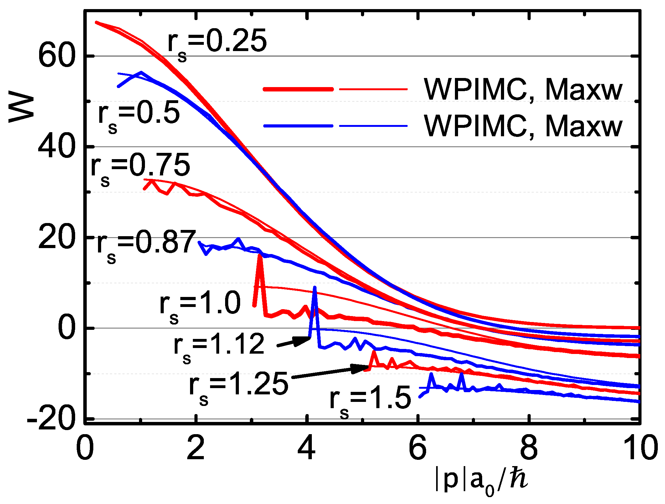
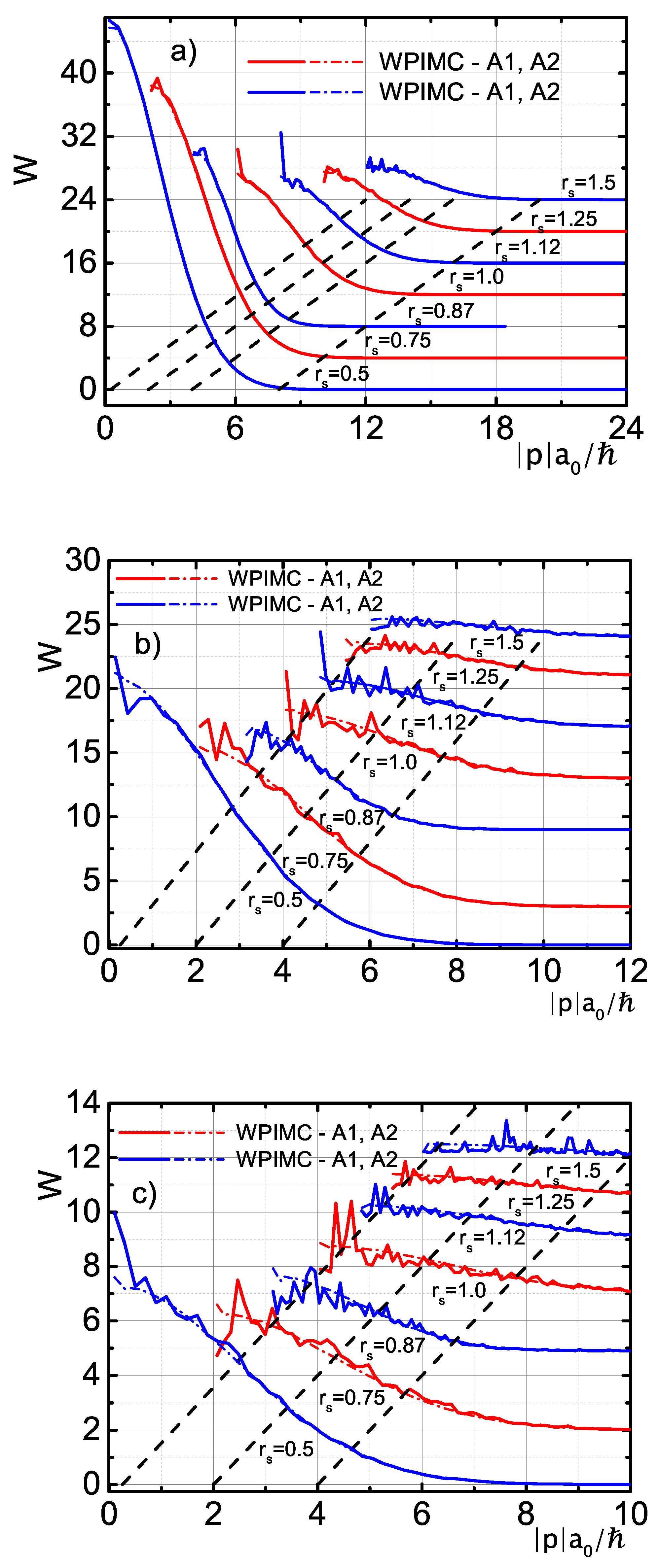
4.1. Momentum Distribution Functions

Figure 1 presents the WPIMC calculations of the UEG electron MDFs. The vertical and horizontal axes show characteristic scales. For convenient comparison, the origins of distributions are shifted along both axes (see Tables S1–S6 in the Supplementary Materials for all Figures). The dashed black lines signify the shifted positions of the characteristic values of momentum $|p|a_0/\hslash$ on the Figure 4. Here, all MDFs are normalized to temperature dependent values equal to ${(2\pi a_0/\lambda )}^3={(\pi /\beta \mathrm{Ry})}^{(3/2)}$.

Let us stress that for a fixed $\theta$ with increasing density, the physical temperature increases and the MDF is approaching the Maxwell distribution (MD) (line $r_s=0.25$, $W_{Mxw}$∼$exp[-{(p\lambda /\hslash )}^2/4\pi ]$). Moreover, at large momentum in asymptotic regions the WPIMC MDF and Maxwell momentum distributions practically coincide. At smaller momentum and intermediate density the WPIMC MDFs show two types of peaks disturbing the Maxwell momentum distribution function: small irregular peaks characterizing the statistical error of WPIMC calculations and the narrow high individual peaks, whose physical meaning must be analyzed.

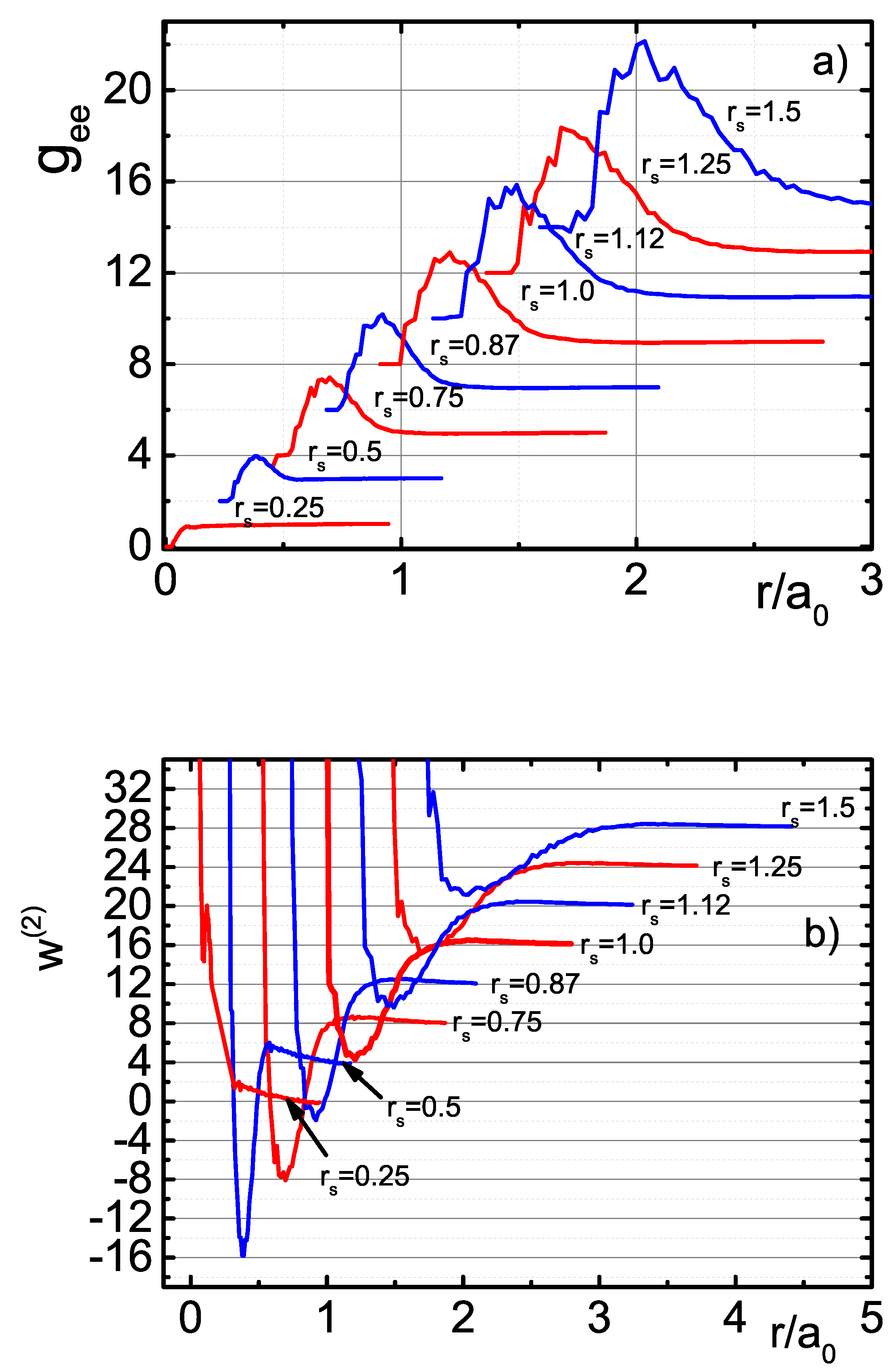
4.2. Pair Distribution Functions and Potential of the Mean Force

We are going to consider the peaks in the electron pair distribution functions (PDF) associated with the exchange-correlation excitons [27] and the sharp high picks in the momentum distribution functions (MDF) to check the existence of the corresponding electron bound states. To do this, let us start from the analysis of a potential of the mean force (PMF) [13] defined by the electron–electron PDF. The potential of the mean force ought to reproduce the correct radial distribution function in PIMC simulations.

The potential of mean force $w^{(n)}$ [13] of a system with N classical particles is defined as

$$\begin{array}{c}\hfill -{\nabla }_j{w}^{(n)}=\frac{\int e^{-\beta U}(-{\nabla }_{j}U)d{q}_{n+1}\dots d{q}_N}{\int e^{-\beta U}d{q}_{n+1}\dots d{q}_N},j=1,2,\dots ,n.\end{array}$$

(19)

Above, $-{\nabla }_j{w}^{(n)}$ is the averaged force, i.e., the “mean force” acting on particle j. For $n=2$$w^{(2)}$ is related to the radial distribution function of the system as

$$\begin{array}{c}\hfill g(r)=e^{-\beta w^{(2)}(r)}.\end{array}$$

(20)

Here, the PDF $g(r)$ for a binary mixture of electrons and positive particles can be written in the form [13,28],

$$\begin{array}{c}\hfill g_{ab}(r)=g_{ab}(R_1,R_2)=\sum _{\sigma }\underset{V}{\int }\mathrm{d}x\delta (R_1-x_{1,a})\delta (R_2-x_{2,b})\rho (x,\sigma ;\beta )/Z(N_e,N_p,V,\beta )\end{array}$$

(21)

where $r=R_1-R_2$, a, and b label the particle species.

Figure 2a presents the WPIMC calculations of the electron–electron PDFs, while Figure 2b shows the corresponding PMFs in atomic units. As previously, for convenient comparison the origins of the distributions and PMFs are shifted along both axes. With increasing density for a fixed $\theta$, the characteristic PDF height becomes smaller while the PDF width becomes narrower. Respectively, the depth of the PMF is increasing while the width of the PMF is decreasing. Peaks in PDFs can be associated with the exchange-correlation excitons [11,12] arising due to the occurrence of the exchange positively charged hole and the excluded volume effect [29]. This effect is a consequence of the interference effects of Coulomb and exchange interactions of electrons.

4.3. Bound States and the Energy Levels

Let us analyze the physical consequences of the above-mentioned behavior of the PMF. The semiclassical approximation used here turned out to be very effective for many issues of quantum mechanics and mathematical physics.

The fundamental difference between a one-dimensional potential well from a three-dimensional system is that for a one-dimensional potential well there is always at least one energy level with an even wave function. In the case of a spherically symmetric potential well $w^2$, this may not be the case. Let us consider a simple criterion for the existence of bound states [15]:

$$\begin{array}{c}\hfill B=w_{min}^{(2)}{r}_0^2-\pi /8\le 0,\end{array}$$

(22)

where $w_{min}^{(2)}$ is the minimal value of $w^{(2)}$ and both $w_{min}^{(2)}$ and $r_0$ are taken in atomic units. Here $r_0$ is the radius of a spherical potential well. Under this condition, not a single level of the discrete spectrum will appear (as the depth of the potential well is too shallow).

Values B presented in the caption to Figure 2b demonstrates that at $\Theta =4$, bound states can exist only at low enough density corresponding to $r_s\ge 0.5$. At higher density ($r_s\le 0.5$), bound states can be destroyed by “pressure ionization” similar to plasma.

For more accurate semiclassical estimations let us use the Bohr–Sommerfeld condition for a particle in a spherically symmetric field $w^{(2)}$. The Schrödinger equations for the radial part $R(r)$ of the wave function looks like:

$$\begin{array}{c}\hfill -\frac{1}{2}{R}^{″}+\left[w^{(2)}(r)+\frac{l(l+1)}{2r^2}\right]R=E_{l}R\end{array}$$

(23)

where $E_l$ is the total energy of the particle, $l=0,1,2,\dots$ is the orbital quantum number [15]. In the semiclassical approximation for a particle in the field $w^{(2)}$, the Bohr–Sommerfeld condition takes the form:

$$\begin{array}{c}\hfill \underset{r_1(E)}{\overset{r_2(E)}{\int }}p(r)\mathrm{d}r=\pi \left(n_r+\frac{1}{2}\right)\end{array}$$

(24)

where for any energy $E\ge w_{min}^{(2)}$, there are only two turning points, $r_1$ and $r_2$, and

$$\begin{array}{c}\hfill p=p(r)=\sqrt{2[E_l-w^{(2)}(r)]-\frac{{(l+\frac{1}{2})}^2}{r^2}},\end{array}$$

(25)

where $n_r$ is the number of zeros of the radial function [15].

Figure 3 presents the average energy levels obtained according to the semiclassical Bohr–Sommerfeld condition (24) with $n_r=0$ in the range of densities related to $r_s$ from 0.87 up to 1.50. The obtained results show that the bound states with negative energy tend to zero at increasing density and then the bound states disappear.

To check the disturbance of the momentum distribution functions by the bound states, let us estimate the related values of momenta. To do this, we use the equation for the spherical potential well $p{a}_0/\hslash =\sqrt{2(|E|/\mathrm{Ha})/(r_0/a_0)}$. We can see that the sharp peaks of the MDF at $p{a}_0/\hslash \sim 0$ and $p{a}_0/\hslash \sim 1$ correspond to the bound states with $|E|/\mathrm{Ha}\sim 0$, $|E|/\mathrm{Ha}\sim 1-2$ and $r_0/a_0\sim 1$ (see Figure 2), which are demonstrated in Figure 1 and Figure 4 for $\Theta =4$, $\Theta =2$, $\Theta =1$.

Figure 4 demonstrates the noticeable repetition in position of the sharp similar peaks in the MDF for neighboring densities and temperatures. For example, in Figure 4c there are two series of high similar peaks presented by lines related to $r_s=0.5$, $r_s=0.75$, $r_s=0.87$ and $r_s=1$, $r_s=1.12$, $r_s=1.25$, respectively. Let us note that lines $r_s=1$, and $r_s=1.25$ confirm clearly the existence of the bound states with eigenvalues E of the order of two Hartrees. Here the electron momentum distribution functions are affected by a strong interaction of charges.

The appearance of the bound states is the physical reason of the peaks in the electron MDFs. These results also reveal the density-temperature range of the exchange-correlation exciton arising, existence, and decay.

To analyze the influence of interparticle interaction on the exchange interaction and the properties of the UEG we have compared the obtained results for Equation (10) (marked by A1) to those (marked by A2) for: ${\varphi }_{kt}=exp\{-\pi {\left|r_{kt}\right|}^2/M\}$. In Figure 4, the MDF for case A2 has no sharp peaks and demonstrates only smooth small oscillations related to statistical errors of the WPIMC calculations. The expression A1 in comparison with approximation A2 accounts for more accurately the Coulomb and Fermi repulsion of electrons, which result in the occurrence of the peaks in MDFs and PDFs.

5. Discussion and Conclusions

The representation of the Wigner function developed in this paper allows us to account for the impact of the interparticle interaction on the Pauli exclusion principle of fermions, as well as to reduce the “sign problem” and to calculate the momentum distribution functions that are inaccessible to the standard PIMC methods.

The obtained pair electron–electron distribution functions for the UEG demonstrate the short-range quantum ordering of electrons associated in the literature with the exchange-correlation excitons. The presented results allow us to estimate the density-temperature range of arising, existence, and decay of the exchange-correlation excitons. This fine physical effect was not observed earlier in standard path integral Monte Carlo simulations.

The physical analysis of the electron bound states in excitons was done in the framework of the semiclassical Bohr–Sommerfeld quantization condition applied to the potentials of the mean force arising from the corresponding pair electron–electron distribution functions. We demonstrated the existence of the electron bound states disturbing the Maxwellian distribution and estimated the averaged energy levels.

The electron MDF of the mixture of free electrons and exchange-correlation excitons is characterized by narrow sharp peaks in contrast to the monotonic Maxwellian distribution. A qualitative explanation of the MDF behavior averaged over all electrons is as follows: the MDF of the free electrons and the center of mass of the excitons is Maxwellian, with the average momentum of the order of $(5-10)p{a}_0/\hslash$ at considered temperatures. As it follows from the behavior of PMF in Figure 2b and the Bohr–Sommerfeld condition, the electron momentum of the bound states in the center of mass is of the order of $p{a}_0/\hslash$∼1. The total electron momentum of the exciton is the sum of the center of mass momentum and the relative one to the center of the mass. So, the electron MDF averaged over the excitons with the center of mass momentum $p{a}_0/\hslash \gg 1$ have to coincide with the Maxwellian distribution, as the bound state peaks in the distribution will be smoothed by the Brownian motion. At the same time, for slow electrons and excitons with the center of mass $p{a}_0/\hslash$∼1, the Maxwellian distribution has to be explicitly disturbed by the bound state peaks, as demonstrated in Figure 4, for the MDF averaged over all electrons.

The noticeable repetition in position of the series of similar sharp peaks in the MDF for neighboring densities and temperatures in independent WPIMC calculations confirms the reliability of the obtained results and the average structure of energy levels.

References

1. Feynman, R.P.; Hibbs, A.R. Quantum Mechanics and Path Integrals; Mcgraw-Hill Book Company: New York, NY, USA, 1965. [Google Scholar]
2. Zamalin, V.; Norman, G.; Filinov, V. The Monte Carlo Method in Statistical Thermodynamics; Nauka: Moscow, Russia, 1977. [Google Scholar]
3. Ebeling, W.; Fortov, V.; Filinov, V. Quantum Statistics of Dense Gases and Nonideal Plasmas; Springer: Berlin/Heidelberg, Germany, 2017. [Google Scholar]
4. Fortov, V.; Filinov, V.; Larkin, A.; Ebeling, W. Statistical Physics of Dense Gases and Nonideal Plasmas; PhysMatLit: Moscow, Russia, 2020. [Google Scholar]
5. Wigner, E. On the interaction of electrons in metals. Phys. Rev. 1934, 46, 1002. [Google Scholar] [CrossRef]
6. Tatarskii, V.I. The Wigner representation of quantum mechanics. Sov. Phys. Uspekhi 1983, 26, 311. [Google Scholar] [CrossRef]
7. Filinov, V.; Larkin, A.; Levashov, P. Uniform electron gas at finite temperature by fermionic-path-integral Monte Carlo simulations. Phys. Rev. E 2020, 102, 033203. [Google Scholar] [CrossRef]
8. Giuliani, G.; Vignale, G. Quantum Theory of the Electron Liquid; Cambridge University Press: Cambridge, UK, 2005. [Google Scholar]
9. Mahan, G. Many-Particle Physics; Plenum Press: New York, NY, USA, 1990. [Google Scholar]
10. Dornheim, T.; Groth, S.; Bonitz, M. The uniform electron gas at warm dense matter conditions. Phys. Rep. 2018, 744, 1–86. [Google Scholar] [CrossRef] [Green Version]
11. Himpsel, F. The Exchange Hole in the Dirac Sea. arXiv 2017, arXiv:1701.08080. [Google Scholar]
12. Weisskopf, V.F. On the self-energy and the electromagnetic field of the electron. Phys. Rev. 1939, 56, 72. [Google Scholar] [CrossRef]
13. Kirkwood, J.G. Statistical mechanics of fluid mixtures. J. Chem. Phys. 1935, 3, 300–313. [Google Scholar] [CrossRef]
14. Hagedorn, G.A.; Robinson, S.L. Bohr–Sommerfeld quantization rules in the semiclassical limit. J. Phys. A Math. Gen. 1998, 31, 10113. [Google Scholar] [CrossRef]
15. Nikiforov, A.F.; Novikov, V.G.; Uvarov, V.B. Quantum-Statistical Models of Hot Dense Matter: Methods for Computation Opacity and Equation of State; Springer Science & Business Media: Berlin/Heidelberg, Germany, 2005; Volume 37. [Google Scholar]
16. Zamalin, V.; Norman, G. The Monte-Carlo method in Feynman’s formulation of quantum statistics. USSR Comput. Math. Math. Phys. 1973, 13, 169–183. [Google Scholar] [CrossRef]
17. Larkin, A.; Filinov, V. Phase space path integral representation for wigner function. J. Appl. Math. Phys. 2017, 5, 392–411. [Google Scholar] [CrossRef] [Green Version]
18. Larkin, A.; Filinov, V.; Fortov, V. Path integral representation of the Wigner function in canonical ensemble. Contrib. Plasma Phys. 2016, 56, 187–196. [Google Scholar] [CrossRef]
19. Wiener, N. Differential-space. J. Math. Phys. 1923, 2, 131–174. [Google Scholar] [CrossRef]
20. Kelbg, G. Theorie des Quanten-Plasmas. Ann. Phys. 1963, 457, 354. [Google Scholar] [CrossRef]
21. Ebeling, W.; Hoffmann, H.; Kelbg, G. Quantenstatistik des Hochtemperatur-Plasmas im thermodynamischen Gleichgewicht. Beitr. Plasmaphys. 1967, 7, 233–248. [Google Scholar] [CrossRef]
22. Filinov, A.; Golubnychiy, V.; Bonitz, M.; Ebeling, W.; Dufty, J.W. Temperature-dependent quantum pair potentials and their application to dense partially ionized hydrogen plasmas. Phys. Rev. E 2004, 70, 04641. [Google Scholar] [CrossRef] [PubMed] [Green Version]
23. Ebeling, W.; Filinov, A.; Bonitz, M.; Filinov, V.; Pohl, T. The method of effective potentials in the quantum-statistical theory of plasmas. J. Phys. A Math. Gen. 2006, 39, 4309. [Google Scholar] [CrossRef]
24. Klakow, D.; Toepffer, C.; Reinhard, P.G. Semiclassical molecular dynamics for strongly coupled Coulomb systems. J. Chem. Phys. 1994, 101, 10766–10774. [Google Scholar] [CrossRef]
25. Larkin, A.; Filinov, V.; Fortov, V. Peculiarities of the momentum distribution functions of strongly correlated charged fermions. J. Phys. A Math. Theor. 2017, 51, 035002. [Google Scholar] [CrossRef] [Green Version]
26. Huang, K. Statistical Mechanics; John Wiley & Sons: Hoboken, NJ, USA, 1963. [Google Scholar]
27. Filinov, V.; Levashov, P.; Larkin, A. Monte Carlo simulations of the electron short-range quantum ordering in Coulomb systems and the “fermionic sign problem”. J. Phys. A Math. Theor. 2021, 55, 035001. [Google Scholar] [CrossRef]
28. Fisher, I.Z. Statistical Theory of Liquids; University of Chicago Press: Chicago, IL, USA, 1964. [Google Scholar]
29. Barker, J.; Henderson, D. Theories of liquids. Annu. Rev. Phys. Chem. 1972, 23, 439–484. [Google Scholar] [CrossRef]
Figure 1. (Color online) The UEG electron momentum distribution functions W ( | p | a 0 / ) normalized to ( π / β Ry ) ( 3 / 2 ) at Θ = 4 . Thick lines—WPIMC distributions, thin lines—Maxwell–Boltzmann distributions. For better representation, W ( | p | a 0 / ) for r s = 0.25 and r s = 0.5 are divided by 14 and 2, respectively.
Universe 08 00079 g001
Figure 2. (Color online) (a) The UEG electron PDFs g e e ( | r | / a 0 ) and (b) the potential of mean force w ( 2 ) ( r / a 0 ) at Θ = 4 ; g e p and g p p in the considered UEG model are identically equal to unity. For r s = 0.5 B = 0.38 ; for r s = 0.75 B = 2.2 ; for r s = 0.87 B = 0.97 ; for r s = 1 B = 6.11 ; for r s = 1.12 B = 6.15 ; for r s = 1.25 B = 7.5 ; for r s = 1.5 B = 7.82 . The positive or negative values of B are obtained from the criterion of bound states existence (22).
Universe 08 00079 g002
Figure 3. (Color online) Some average exciton energy levels at orbital quantum number l = 0 (blue circles) and at l = 1 (red circles) for Θ = 4 . Circles: 1— E 0 = 0.08 at r s = 0.75 ; 2— E 0 = 1 and E 0 = 0.10 at r s = 0.87 ; 3— E 0 = 1.75 and E 0 = 0.15 at r s = 1 ; 4– E 0 = 2.22 and E 1 = 0.8 at r s = 1.12 ; 5— E 0 = 2.25 and E 1 = 0.50 at r s = 1.25 ; 6— E 0 = 2.25 and E 1 = 0.05 at r s = 1.50 .
Universe 08 00079 g003
Figure 4. (Color online) The UEG electron momentum distribution functions W ( | p | a 0 / ) at Θ = 4 —(a), Θ = 2 —(b) and Θ = 1 —(c). Solid lines—WPIMC A1, dot-and-dash lines—WPIMC A2. For convenient representation all W ( | p | a 0 / ) for r s = 0.5 are divided by two.
Universe 08 00079 g004
Publisher’s Note: MDPI stays neutral with regard to jurisdictional claims in published maps and institutional affiliations.