Periodic Orbits of the Restricted Three-Body Problem Based on the Mass Distribution of Saturn’s Regular Moons

Abstract

This paper uses the Kolmogorov–Smirnov test to perform a fitting analysis on the mass data of Saturn’s regular moons and found that the lognormal distribution is its best-fitting distribution with an extremely high p-value of 0.9889. Moreover, novel dynamic equations for the variable-mass restricted three-body problem are established based on the newly discovered distribution of mass data, rather than the empirical Jeans’ law, and the Lindstedt–Poincaré perturbation method was used to give the approximate analytical periodic orbits near the Lagrangian point $L_3$. Furthermore, this paper also discusses the influence of the three-body gravitational interaction parameter, the variable-mass parameter of the third body, and the scale parameter in the statistical results on the periodic orbits and the position of the Lagrangian point $L_3$ through numerical simulation.

1. Introduction

Humanity will be challenged by the threat of resource shortages in the future. Some small celestial bodies, planets, and moons may become a breakthrough for obtaining resources. In October 2019, the Sheppard team of the Carnegie Institution in the United States announced the discovery of 20 new moons of Saturn [1]. To date, the Saturn family has 82 members, making it the planet with the largest number of moons in the solar system (see [2] for specific classification). These natural satellites are divided into regular and irregular moons based on their distance from Saturn, orbital eccentricity, and inclination. From their dynamic behavior and the composition and structure of matter, the Saturnian system is similar to a miniature solar system. For example, scientists discovered an atmosphere and liquid water on Titan. Some scientists have thought that the moon might be an asteroid captured by its host star or the debris produced by its parent body or other moons colliding together [3]. The sources of collisions are diverse, such as main belt asteroids and various comets [3,4]. Dorofeeva [5] believed that the original matter that composes the regular moon Enceladus came from a particular comet, and Castillo-Rogez et al. [6] considered that Phoebe came from a library of C-type asteroids. Gao et al. [7,8] conducted a fitting distribution study on the irregular moon distribution of Jupiter. According to the p-value obtained by the Kolmogorov–Smirnov (K-S) test, they proposed that the log-logistic distribution is the best distribution of their main physical characteristics. The best distribution model inferred from the data can help predict unknown moon physical properties and even help humans discover new natural satellites.

In celestial mechanics, the restricted three-body model describes the motion of an object with a relatively infinitely small mass under the gravitational force of two finite-mass bodies (that is, the main star). It is called the circular restricted three-body problem if the finite mass bodies move in a uniform circular motion around their mass center. This model can approximate the local dynamics of planets or moons with small orbital eccentricities. Considering that the mass and radiation of celestial bodies are constantly changing in practical problems, this has prompted scholars to study the variable-mass three-body problem that is more in line with the actual situation. Therefore, considering variable mass, radiation, albedo, etc., in the restricted three-body problem will be more realistic [9,10,11,12,13,14,15,16,17,18,19,20,21,22]. For example, if a star has a strong radiation ability, the dynamic equation established by ignoring its radiation factor will become unreliable. However, we must admit that the interference of multiple perturbation factors will also complicate the problem, which is not conducive to our study of the influence of certain perturbation factors on the system’s dynamic behavior. Bosanac et al. [23] and Suraj et al. [24] improved the circular restricted three-body problem, that is considering the existence of the three-body interaction, and studied its related dynamic properties. Since periodic orbits have a wide range of practical application values, many scholars have studied the periodic orbits near the Lagrangian points: Abouelmagd and Guirao [25] explored the existence of Lagrangian points under the effects of the perturbations in Coriolis and centrifugal forces, and it was proven that the orbits of the infinitesimal body around the five Lagrangian points are ellipses; Poddar and Sharma [26] proved the existence of periodic orbits when the third coordinate of the infinitesimal mass is zero; Abouelmagd et al. [27] obtained the second-order approximate periodic orbit near the Lagrangian point; Gao [11] also studied the degree of coincidence between the second- and third-order periodic orbits and analyzed the influence of parameter changes on the periodic orbits; Qian [28] obtained the periodic orbit near the triangular Lagrangian points through the polynomial expansion method. Due to the rapid development of computer technology, more researchers have discovered the important periodic orbits of the three-body problem through numerical methods; see [29,30,31,32] for details. Moreover, Yang et al. [33] proposed an artificial-neural-network-based model to improve the computing efficiency.

Inspired by the above references, this article considers the Sun–Saturn-third body model. The third body has a varying mass and can be regarded as the “parent body” of the moons of Saturn, but its mass is negligible compared to the Sun and Saturn. This paper mainly focuses on the approximately analytical periodic orbit around the Lagrangian point and the influence of the three-body interaction parameter and the variable mass parameters of the third body on this orbit. Compared with the references mentioned above, the most significant feature of this paper is that we consider the distribution law of the mass of the actual Saturn moons and then establish a new restricted three-body problem model based on this law. The structure of this paper is as follows: Section 2 uses the K-S test method in statistical inference to give the best-fitting distribution of regular moon mass data. The corresponding restricted three-body dynamic control equation is established based on the distribution law of moon mass data, and the approximate analytic periodic orbit around the Lagrangian point is calculated in Section 3. In Section 4, the influence of the scale parameters of the mass distribution of Saturn’s moons, the three-body interaction parameter, and the varying mass ratio of the moons on the periodic orbits around the Lagrangian point are discussed. The last section is the conclusions.

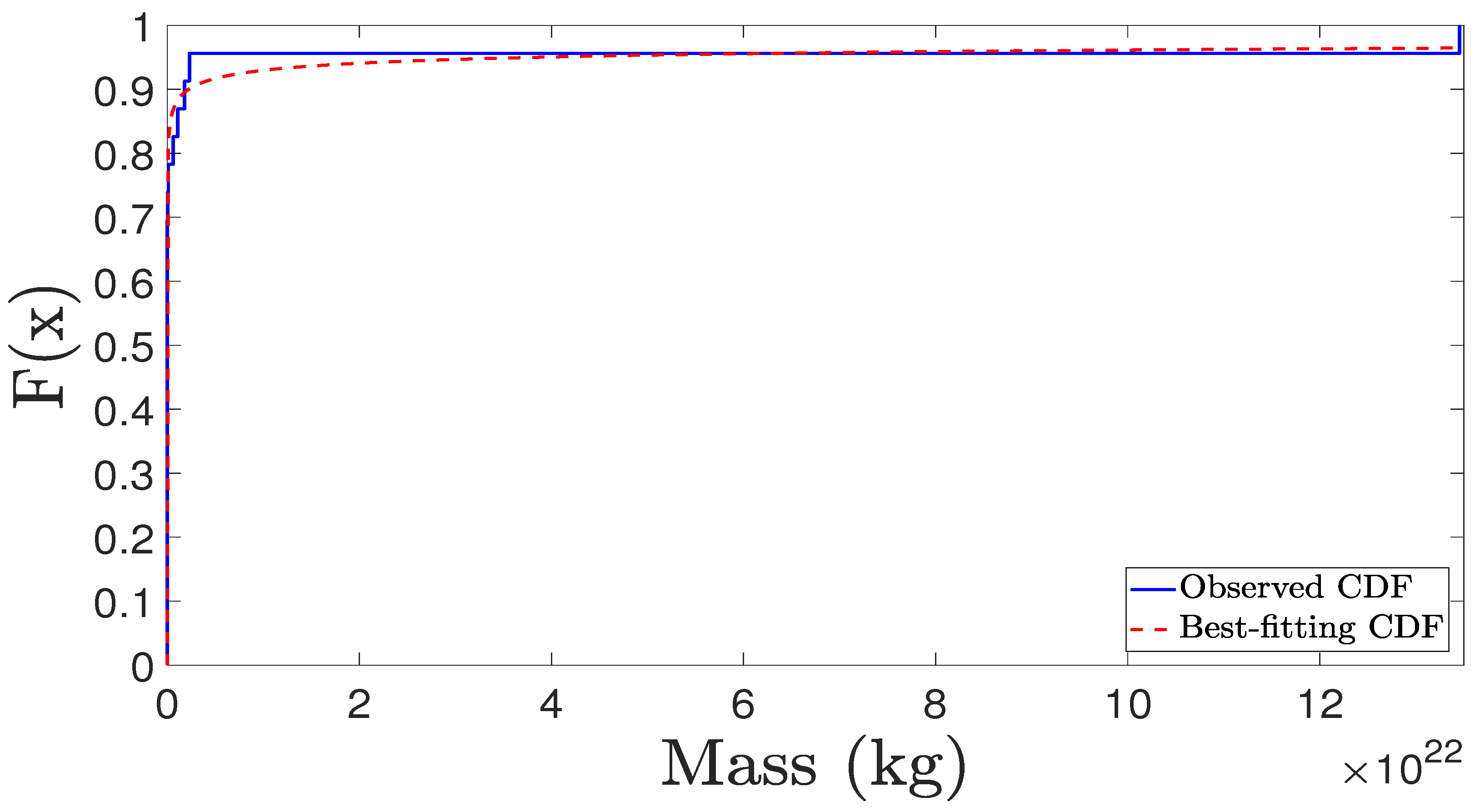
2. Best-Fitting Distribution of the Regular Moons’ Mass

To explore whether the mass data of Saturn’s regular moons (see

Table 1. Mass data of Saturn’s regular moons.

Names of Saturn’s Regular Moons	Mass (kg)	Names of Saturn’s Regular Moons	Mass (kg)
Aegaeon	59,946,737,324	Methone	8,992,010,598,583
Anthe	1,498,668,433,097	Mimas	37,505,676,206,690,400,000
Atlas	6,594,141,105,627,650	Pallene	32,970,705,528,138
Calypso	2,547,736,336,265,230	Pan	4,945,605,829,220,740
Daphnis	77,930,758,521,054	Pandora	138,476,963,218,181,000
Dione	1,095,745,430,185,280,000,000	Polydeuces	4,496,005,299,292
Enceladus	107,944,591,230,692,000,000	Prometheus	160,956,989,714,639,000
Epimetheus	526,032,620,017,115,000	Rhea	2,307,089,151,289,080,000,000
Helene	11,389,880,091,538,700	S/2009 S1	——
Hyperion	5,585,537,250,153,240,000	Telesto	4,046,404,769,362,420
Iapetus	1,805,952,411,282,580,000,000	Tethys	617,551,805,221,061,000,000
Janus	1,892,818,231,001,750,000	Titan	134,552,523,083,241,000,000,000

) have statistical regularity, this section uses the single-sample K-S test to evaluate the mass data of the regular moons. The K-S test is a method to test whether a certain set of sample data comes from a specific distribution. The main idea of this test method is to compare the empirical distribution function of the sample data with the selected theoretical distribution function and check whether the sample data come from this theoretical distribution function according to the difference between the two. The main steps of the test are as follows: first, set the null hypothesis ${\mathrm{H}}_0$: the sample data obey a particular distribution, then the alternative hypothesis ${\mathrm{H}}_1$: the sample data do not obey the particular distribution. Suppose we use $D=max|F_n\left(x\right)-F_0\left(x\right)|$ to represent the maximum value of the gap between the empirical distribution function $F_n\left(x\right)$ and the theoretical distribution function $F_0\left(x\right)$ of the sample data. In that case, the critical value $D(n,\alpha )$ is determined by the number of known sample data n and the significance level $\alpha$, and if the value of D falls within the rejection range, the null hypothesis is rejected. Otherwise, the null hypothesis is not rejected.

In the hypothesis-testing problem, relative to the D-value, the p-value ($0\le p\le 1$) can also reflect the credibility of statistical inference. The p-value is the minimum significance level that can reject the null hypothesis ${\mathrm{H}}_0$ in the hypothesis-testing problem. In other words, the p-value is the probability of falsely rejecting the null hypothesis ${\mathrm{H}}_0$, which is called a Type 1 error. The null hypothesis may become more significant as the p-value increases and decrease as the p-value decreases. When the p-value is smaller than the selected significance level $\alpha$ (this article selected $\alpha =0.05$ according to international practice), the null hypothesis ${\mathrm{H}}_0$ is considered invalid. That is, the sample data do not obey the given theoretical distribution. When multiple distribution functions can fit the same sample data, the distribution function with the most significant p-value can be used as the best-fitting distribution of the sample data. For the mass data of Saturn’s regular moons, a total of 22 common distribution functions were fit in this section, and the specific fitting results are shown in

Table 2. Statistical inference results of the mass of Saturn’s regular moons.

		Beta	Birnbaum– Saunders	Burr	Exponential	Extreme Value	Gamma	Generalized Extreme Value	Generalized Pareto	Half Normal	Inverse Gaussian	Logistic
Mass ($kg$)	h	null	1	0	1	1	0	1	0	1	1	1
	p		0.0345	0.8643	0.0000	0.0000	0.3145	0.0000	0.1723	0.0000	0.0000	0.0000
	parameter		$\beta$ = 8.9038 × ${10}^{16}$ $\gamma$ = 370.466	$\alpha$ = 3.76388 × ${10}^{20}$ c = 0.170255 k = 2.83657	$\mu$ = 6.11012 × ${10}^{21}$	$\mu$ = 2.40706 × ${10}^{22}$ $\sigma$ = 4.92323 × ${10}^{22}$	a = 0.0760157 b = 8.03796 × ${10}^{22}$	k = 0.569397 $\sigma$ = 1.32889 × ${10}^{16}$ $\mu$ = 7.07519 × ${10}^{15}$	k = 11.3686 $\sigma$ = 1.55618 × ${10}^{13}$ $\theta$ = 0	$\mu$ = 0 $\sigma$ = 2.8064 × ${10}^{22}$	$\mu$ = 6.11012 × ${10}^{21}$ $\lambda$ = 1.29748 × ${10}^{12}$	$\mu$ = 6.11012 × ${10}^{21}$ $\sigma$ = 1.54407 × ${10}^{22}$
	confidence interval		$\beta$∈ [3.5716 × ${10}^{16}$, 1.4236 × ${10}^{17}$] $\gamma$ ∈ [263.409, 477.524]	$\alpha$∈ [664.59, 2.13166 × ${10}^{38}$] c ∈ [0.0739575, 0.39194] k ∈ [0.0204874, 392.734]	$\mu$∈ [4.21915 × ${10}^{21}$, 9.63871 × ${10}^{21}$]	$\mu$∈ [2.54927 × ${10}^{21}$, 4.5592 × ${10}^{22}$] $\sigma$ ∈ [3.85631 × ${10}^{22}$, 6.28534 × ${10}^{22}$]	a∈ [0.049786, 0.116065] b ∈ [1.72057 × ${10}^{22}$, 3.75508 × ${10}^{23}$]	k∈ [0.494556, 0.644238] $\sigma$ ∈ [7.47124 × ${10}^{15}$, 2.36367 × ${10}^{16}$] $\mu$ ∈ [1.14168 × ${10}^{15}$, 1.30087 × ${10}^{16}$]	k∈ [6.12161, 16.6156] $\sigma$ ∈ [1.31349 × ${10}^{12}$, 1.84372 × ${10}^{14}$] $\theta$ = 0	$\mu$ = 0 $\sigma$ ∈ [2.18117 × ${10}^{22}$, 3.93671 × ${10}^{22}$]	$\mu$∈ [−Inf,Inf] $\lambda$ ∈ [−Inf,Inf]	$\mu$∈ [−Inf,Inf] $\sigma$ ∈ [−Inf,Inf]
		Log-logistic	Lognormal	Nakagami	Negative Binomial	Normal	Poisson	Rayleigh	Rician	t Location- Scale	Weibull	Stable
Mass($kg$)	h	0	0	0	null	1	1	1	1	1	0	1
	p	0.9759	0.9889	0.2574		0.0000	0.0000	0.0000	0.0000	0.0000	0.7818	0.0000
	parameter	$\mu$ = 39.1312 $\sigma$ = 4.58867	$\mu$ = 39.1272 $\sigma$ = 7.82406	$\mu$ = 0.0357998 $\omega$ = 7.8759 × ${10}^{44}$		$\mu$ = 6.11012 × ${10}^{21}$ $\sigma$ = 2.80064 × ${10}^{22}$	$\lambda$ = 6.11012 × ${10}^{21}$	B = 1.98443 × ${10}^{22}$	s = 1 $\sigma$ = 2.71315 × ${10}^8$	$\mu$ = −1.54662 × ${10}^{15}$ $\sigma$ = 1.81001 × ${10}^{16}$ $\nu$ = 0.177628	A = 4.42076 × ${10}^{18}$ B = 0.142598	$\alpha$ = 0.4 $\beta$ = 0.987279 c = 3.62044 × ${10}^{18}$ $\mu$ = 2.24553 × ${10}^{18}$
	confidence interval	$\mu$∈ [35.7976, 42.4648] $\sigma$ ∈ [3.29169, 6.39669	$\mu$∈ [35.7438, 42.5106] $\sigma$ ∈ [6.05109, 11.0738]	$\mu$∈ [0.0236219, 0.0542557] $\omega$ ∈ [9.08296 × ${10}^{43}$, 6.82924 × ${10}^{45}$]		$\mu$∈ [−6.00076 × ${10}^{21}$, 1.8221 × ${10}^{22}$] $\sigma$ ∈ [2.166 × ${10}^{22}$, 3.96389 × ${10}^{22}$]	$\lambda$∈ [6.11012 × ${10}^{21}$, 6.11012 × ${10}^{21}$]	B∈ [1.64901 × ${10}^{22}$, 2.49241 × ${10}^{22}$]	s = 1 $\sigma$ ∈ [2.71315 × ${10}^8$, 2.71315 × ${10}^8$]	$\mu$∈ [−Inf,Inf] $\sigma$ ∈ [−Inf,Inf] $\nu$ ∈ [−Inf,Inf]	A∈ [2.12356 × ${10}^{17}$, 9.20299 × ${10}^{19}$] B ∈ [0.104361, 0.194845]	$\alpha$∈ [0,2] $\beta$ ∈ [−1,1] c ∈ [0,Inf] $\mu$ ∈ [−Inf,Inf]

. It is not difficult to find that the maximum p-value can reach 0.9889; the corresponding best-fitting distribution is the lognormal distribution, and its probability density function (PDF) is:

$$f\left(x\right)=\frac{1}{x\sqrt{2\pi }\sigma }exp\frac{-{(lnx-\mu )}^2}{2{\sigma }^2};$$

(1)

the PDF of the normal distribution corresponding to this distribution is:

$$f(lnx)=\frac{1}{\sqrt{2\pi }\sigma }exp\frac{-{(lnx-\mu )}^2}{2{\sigma }^2}.$$

(2)

Here, the location parameter $-\infty <\mu <+\infty$ is the mean of the logarithmic value, and the scale parameter $\sigma \ge 0$ is the standard deviation of the logarithmic value. The lognormal distribution is sometimes called the Galton distribution, which can be obtained after logarithmic transformation of the normal distribution. It should be noted that the lognormal distribution requires that each datum X be a positive number because $ln\left(X\right)$ is meaningful only when $X>0$. If X follows the lognormal distribution with parameters $\mu$ and $\sigma$, then $ln\left(X\right)$ follows the normal distribution with mean $\mu$ and standard deviation $\sigma$. Similarly, if X follows the normal distribution with parameters $\mu$ and $\sigma$, then $exp\left(X\right)$ obeys the lognormal distribution. $\mu$ refers to the position parameter of the lognormal distribution, not the position parameter of Saturn’s regular moons. From the results of statistical inference, the estimated value of parameter $\mu$ in Equations (1) and (2) is 39.1272 with the corresponding confidence interval being [35.7438, 42.5106], and the estimated value of parameter $\sigma$ is 7.82406 with the corresponding confidence interval being [6.05109, 11.0738]. The cumulative distribution function (CDF) of moon mass data and the CDF corresponding to the best-fitting distribution are shown in Figure 1. It is easy to find that the lognormal distribution can fit the mass distribution of Saturn’s regular moons well.

3. Dynamic Equations and Approximate Periodic Orbits

3.1. Dynamic Model with Variable Mass

Based on the law of mass distribution in the previous section, this section mainly analyzes the dynamic behavior of the restricted three-body problem composed of the Sun, Saturn, and the third body with variable mass (the mass is negligible relative to the Sun and Saturn). The third body here can be regarded as the “parent planet” of Saturn’s moons because it has long been suspected that the moons were formed when the larger bodies disintegrated. According to the results of statistical inference, let the mass m of the third body obey the lognormal distribution with the location parameter $\mu$ and the scale parameter $\sigma$; then, $ln\left(m\right)$ obeys the normal distribution with mean $\mu$ and standard deviation $\sigma$. Note that if the mass m of the third body is a function that changes with the evolution time $\tau$, then its probability density expression is:

$$f(lnm\left(\tau \right))=\frac{1}{\sqrt{2\pi }\sigma }exp\frac{-{(lnm\left(\tau \right)-\mu )}^2}{2{\sigma }^2}.$$

(3)

Performing the time scale transformation $t={(lnm\left(\tau \right)-\mu )}^2/2$, we have:

$$\frac{1}{\sqrt{2\pi }\sigma }exp\frac{-t}{{\sigma }^2}\triangleq m\left(t\right),$$

(4)

then:

$$\frac{\mathrm{d}m\left(t\right)}{\mathrm{d}\mathrm{t}}=-\frac{1}{{\sigma }^2}m\left(t\right).$$

(5)

We considered the movement of the third body in the gravitational field of the Sun and Saturn and established a center-of-mass rotating coordinate system O-$UVW$: taking the center-of-mass of the Sun–Saturn system as the origin, the plane of relative motion as the orbital plane, the U axis passing through the line of the Sun and Saturn, the V axis perpendicular to the U axis in the plane of motion, and the W axis passing through the center-of-mass of the Sun–Saturn system and rotating perpendicular to its plane of motion. Normalize related physical quantities. Let the mass of the Sun be $m_1$ and the mass of Saturn be $m_2$; then, the mass ratio parameter $\mu =m_2/(m_1+m_2)\le 1/2$, $m_1=1-\mu$, $m_2=\mu$. Therefore, the dimensionless dynamic equation of the third body can be described as:

$$\begin{array}{cc}\hfill (\ddot{u}-2\dot{v})+\frac{\dot{m}}{m}(\dot{u}-v)& ={\mathsf{\Omega }}_u^{*},\hfill \\ \hfill (\ddot{v}+2\dot{u})+\frac{\dot{m}}{m}(\dot{v}+u)& ={\mathsf{\Omega }}_v^{*},\hfill \\ \hfill \ddot{w}+\frac{\dot{m}}{m}\dot{w}& ={\mathsf{\Omega }}_w^{*},\hfill \end{array}$$

(6)

where the potential energy function is:

$$\begin{array}{c}\hfill {\mathsf{\Omega }}^{*}=\frac{1}{2}\left(u^2+v^2\right)+\frac{(1-\mu )q_1}{{\rho }_1}+\frac{\mu q_2}{{\rho }_2}+\frac{k}{{\rho }_1{\rho }_2},\end{array}$$

(7)

where k is the three-body interaction parameter, ${\rho }_1^2={(u+\mu )}^2+v^2+w^2$ and ${\rho }_2^2={(u-(1-\mu ))}^2+v^2+w^2$ are the distances from the third body to the Sun and Saturn, respectively, and $q_1$ and $q_2$ are the radiation factors of the Sun and Saturn, respectively. For more explanation, please refer to [15,23,24]. To simplify Equation (6), according to the space–time transformation formula:

$$\begin{array}{c}\hfill (\xi ,\eta ,\zeta )={\gamma }^q(u,v,w),\mathrm{d}\mathsf{\Gamma }={\gamma }^l\mathrm{d}\tau ,\end{array}$$

(8)

where $\gamma =m/m_0$ represents the mass ratio and $m_0$ is the mass of the third body at the initial moment. Substituting Equations (5) and (8) into Equation (6) and letting $q=1/2$, $l=0$, Equation (6) becomes:

$$\begin{array}{cc}\hfill \ddot{\xi }-2\dot{\eta }& ={\mathsf{\Omega }}_{\xi },\hfill \\ \hfill \ddot{\eta }+2\dot{\xi }& ={\mathsf{\Omega }}_{\eta },\hfill \\ \hfill \ddot{\zeta }& ={\mathsf{\Omega }}_{\zeta },\hfill \end{array}$$

(9)

where the potential energy function is:

$$\begin{array}{c}\hfill \mathsf{\Omega }=\frac{1}{2}\left({\xi }^2+{\eta }^2\right)+{\gamma }^{\frac{3}{2}}\left[\frac{(1-\mu )q_1}{r_1}+\frac{\mu q_2}{r_2}\right]+\frac{k{\gamma }^2}{r_1{r}_2}+\frac{1}{8{\sigma }^4}\left({\xi }^2+{\eta }^2+{\zeta }^2\right),\end{array}$$

(10)

here $r_1^2={(\xi +\mu {\gamma }^{1/2})}^2+{\eta }^2+{\zeta }^2$, $r_2^2={\left(\xi -(1-\mu ){\gamma }^{1/2}\right)}^2+{\eta }^2+{\zeta }^2$.

3.2. Periodic Orbits near the Lagrangian Point $L_3$

Without loss of generality, we analyzed the periodic orbits around the Lagrangian point $L_3$. Consider the dynamic equations of the third body on the U-V plane:

$$\begin{array}{cc}\hfill \ddot{\xi }-2\dot{\eta }& ={\mathsf{\Omega }}_{\xi },\hfill \\ \hfill \ddot{\eta }+2\dot{\xi }& ={\mathsf{\Omega }}_{\eta },\hfill \end{array}$$

(11)

where:

$$\begin{array}{cc}\hfill {\mathsf{\Omega }}_{\xi }=& -{\gamma }^{\frac{3}{2}}\left[\frac{q_1(1-\mu )(\xi +\mu {\gamma }^{1/2})}{{\left({(\xi +\mu {\gamma }^{1/2})}^2+{\eta }^2\right)}^{\frac{3}{2}}}+\frac{q_2\mu (\xi -(1-\mu ){\gamma }^{1/2})}{{\left({(\xi -(1-\mu ){\gamma }^{1/2})}^2+{\eta }^2\right)}^{\frac{3}{2}}}\right]\hfill \\ \hfill & -\frac{k{\gamma }^2}{{\left({(\xi +\mu {\gamma }^{1/2})}^2+{\eta }^2\right)}^{\frac{1}{2}}{\left({(\xi -(1-\mu ){\gamma }^{1/2})}^2+{\eta }^2\right)}^{\frac{1}{2}}}\left[\frac{\xi +\mu {\gamma }^{1/2}}{{(\xi +\mu {\gamma }^{1/2})}^2+{\eta }^2}\right.\hfill \end{array}$$

(12)

$$\begin{array}{cc}\hfill & \left.+\frac{\xi -(1-\mu ){\gamma }^{1/2}}{{(\xi -(1-\mu ){\gamma }^{1/2})}^2+{\eta }^2}\right]+\xi \left(1+\frac{1}{4{\sigma }^4}\right),\hfill \\ \hfill {\mathsf{\Omega }}_{\eta }=& -{\gamma }^{\frac{3}{2}}\eta \left[\frac{q_1(1-\mu )}{{\left({(\xi +\mu {\gamma }^{1/2})}^2+{\eta }^2\right)}^{\frac{3}{2}}}+\frac{q_2\mu }{{\left({(\xi -(1-\mu ){\gamma }^{1/2})}^2+{\eta }^2\right)}^{\frac{3}{2}}}\right]\hfill \\ \hfill & -\frac{k{\gamma }^2\eta }{{\left({(\xi +\mu {\gamma }^{1/2})}^2+{\eta }^2\right)}^{\frac{1}{2}}{\left({(\xi -(1-\mu ){\gamma }^{1/2})}^2+{\eta }^2\right)}^{\frac{1}{2}}}\left[\frac{1}{{(\xi +\mu {\gamma }^{1/2})}^2+{\eta }^2}\right.\hfill \\ \hfill & \left.+\frac{1}{{(\xi -(1-\mu ){\gamma }^{1/2})}^2+{\eta }^2}\right]+\eta \left(1+\frac{1}{4{\sigma }^4}\right).\hfill \end{array}$$

(13)

By introducing the transformation $\xi ={\xi }_{L_3}+x$ and $\eta =y$, where $({\xi }_{L_3},0)$ is the coordinate of Lagrangian point $L_3$, the dynamic Equation (11) becomes:

$$\begin{array}{cc}\hfill \ddot{x}-2\dot{y}& ={\mathsf{\Omega }}_x,\hfill \\ \hfill \ddot{y}+2\dot{x}& ={\mathsf{\Omega }}_y.\hfill \end{array}$$

(14)

Using Taylor’s formula to expand the right side of Equation (14) to the second- and third-order, respectively, we obtain:

$$\begin{array}{cc}\hfill \ddot{x}-2\dot{y}& =K_{1}x+K_2{x}^2+K_3{y}^2,\hfill \\ \hfill \ddot{y}+2\dot{x}& =P_{1}y+P_{2}xy.\hfill \end{array}$$

(15)

$$\begin{array}{cc}\hfill \ddot{x}-2\dot{y}& =K_{1}x+K_2{x}^2+K_3{y}^2+K_4{x}^3+K_{5}x{y}^2,\hfill \\ \hfill \ddot{y}+2\dot{x}& =P_{1}y+P_{2}xy+P_3{y}^3+P_4{x}^{2}y.\hfill \end{array}$$

(16)

The coefficient expressions of the expansion items above are listed as follows:

$$\begin{array}{ccc}& K_1=\left(1+\frac{1}{4{\sigma }^4}\right)+2{\gamma }^{\frac{3}{2}}\left[\frac{q_1(1-\mu )}{d_{01}^3}+\frac{q_2\mu }{d_{02}^3}\right]+\frac{2k{\gamma }^2}{d_{01}{d}_{02}}\left(\frac{1}{d_{01}^2}+\frac{1}{d_{02}^2}\right)+\frac{2k{\gamma }^2}{d_{01}^2{d}_{02}^2}{V}_1{V}_2,\hfill & \\ & K_2=-{\gamma }^{\frac{3}{2}}\left[\frac{3q_1(1-\mu )}{d_{01}^4}{V}_1+\frac{3q_2\mu }{d_{02}^4}{V}_2\right]-\frac{3k{\gamma }^2}{d_{01}^4{d}_{02}}{V}_1-\frac{3k{\gamma }^2}{d_{01}{d}_{02}^4}{V}_2-\frac{3k{\gamma }^2}{d_{01}^2{d}_{02}^3}{V}_1-\frac{3k{\gamma }^2}{d_{01}^3{d}_{02}^2}{V}_2,\hfill & \\ & K_3=\frac{3}{2}{\gamma }^{\frac{3}{2}}\left[\frac{q_1(1-\mu )}{d_{01}^4}{V}_1+\frac{q_2\mu }{d_{02}^4}{V}_2\right]+\frac{3k{\gamma }^2}{2d_{01}^4{d}_{02}}{V}_1+\frac{3k{\gamma }^2}{2d_{01}{d}_{02}^4}{V}_2+\frac{k{\gamma }^2}{2d_{01}^2{d}_{02}^3}{V}_1+\frac{k{\gamma }^2}{2d_{01}^3{d}_{02}^2}{V}_2,\hfill & \\ & K_4=4{\gamma }^{\frac{3}{2}}\left[\frac{q_1(1-\mu )}{d_{01}^5}+\frac{q_2\mu }{d_{02}^5}\right]+\frac{4k{\gamma }^2}{d_{01}^5{d}_{02}}+\frac{4k{\gamma }^2}{d_{01}^3{d}_{02}^3}+\frac{4k{\gamma }^2}{d_{01}{d}_{02}^5}+\frac{4k{\gamma }^2}{d_{01}^4{d}_{02}^2}{V}_1{V}_2+\frac{4k{\gamma }^2}{d_{01}^2{d}_{02}^4}{V}_1{V}_2,\hfill & \\ & K_5=-6{\gamma }^{\frac{3}{2}}\left[\frac{q_1(1-\mu )}{d_{01}^5}+\frac{q_2\mu }{d_{02}^5}\right]-\frac{6k{\gamma }^2}{d_{01}^5{d}_{02}}-\frac{2k{\gamma }^2}{d_{01}^3{d}_{02}^3}-\frac{6k{\gamma }^2}{d_{01}{d}_{02}^5}-\frac{3k{\gamma }^2}{d_{01}^4{d}_{02}^2}{V}_1{V}_2-\frac{3k{\gamma }^2}{d_{01}^2{d}_{02}^4}{V}_1{V}_2,\hfill & \\ & P_1=\left(1+\frac{1}{4{\sigma }^4}\right)-{\gamma }^{\frac{3}{2}}\left[\frac{q_1(1-\mu )}{d_{01}^3}+\frac{q_2\mu }{d_{02}^3}\right]-\frac{k{\gamma }^2}{d_{01}^3{d}_{02}}-\frac{k{\gamma }^2}{d_{01}{d}_{02}^3},\hfill & \\ & P_2=3{\gamma }^{\frac{3}{2}}\left[\frac{q_1(1-\mu )}{d_{01}^4}{V}_1+\frac{q_2\mu }{d_{02}^4}{V}_2\right]+\frac{3k{\gamma }^2}{d_{01}^4{d}_{02}}{V}_1+\frac{3k{\gamma }^2}{d_{01}{d}_{02}^4}{V}_2+\frac{k{\gamma }^2}{d_{01}^2{d}_{02}^3}{V}_1+\frac{k{\gamma }^2}{d_{01}^3{d}_{02}^2}{V}_2,\hfill & \\ & P_3=\frac{3}{2}{\gamma }^{\frac{3}{2}}\left[\frac{q_1(1-\mu )}{d_{01}^5}+\frac{q_2\mu }{d_{02}^5}\right]+\frac{3k{\gamma }^2}{2d_{01}^5{d}_{02}}+\frac{k{\gamma }^2}{d_{01}^3{d}_{02}^3}+\frac{3k{\gamma }^2}{2d_{01}{d}_{02}^5},\hfill & \\ & P_4=-6{\gamma }^{\frac{3}{2}}\left[\frac{q_1(1-\mu )}{d_{01}^5}+\frac{q_2\mu }{d_{02}^5}\right]-\frac{6k{\gamma }^2}{d_{01}^5{d}_{02}}-\frac{2k{\gamma }^2}{d_{01}^3{d}_{02}^3}-\frac{6k{\gamma }^2}{d_{01}{d}_{02}^5}-\frac{3k{\gamma }^2}{d_{01}^4{d}_{02}^2}{V}_1{V}_2-\frac{3k{\gamma }^2}{d_{01}^2{d}_{02}^4}{V}_1{V}_2,\hfill \end{array}$$

where $d_{01}=\left|u_{L_3}+\mu {\gamma }^{\frac{1}{2}}\right|,d_{02}=\left|u_{L_3}+(\mu -1){\gamma }^{\frac{1}{2}}\right|$ and $V_1=sgn\left(u_{L_3}+\mu {\gamma }^{\frac{1}{2}}\right),V_2=sgn\left(u_{L_3}+(\mu -1){\gamma }^{\frac{1}{2}}\right)$.

Assume that the solutions of Systems (15) and (16) with respect to the perturbation parameter $\epsilon \left(\right|\epsilon |\le 1)$ are expressed as:

$$\begin{array}{cc}\hfill x& =x_1\epsilon +x_2{\epsilon }^2,\hfill \\ \hfill y& =y_1\epsilon +y_2{\epsilon }^2.\hfill \end{array}$$

(17)

$$\begin{array}{cc}\hfill x& =x_1\epsilon +x_2{\epsilon }^2+x_3{\epsilon }^3,\hfill \\ \hfill y& =y_1\epsilon +y_2{\epsilon }^2+y_3{\epsilon }^3.\hfill \end{array}$$

(18)

Substituting Equations (17) and (18) into Equations (15) and (16), respectively, and comparing the degree of parameter $\epsilon$, we have:

$${\epsilon }^1:\left\{\begin{array}{cc}\hfill {\ddot{x}}_1-2{\dot{y}}_1& =K_1{x}_1,\hfill \\ \hfill {\ddot{y}}_1+2{\dot{x}}_1& =P_1{y}_1.\hfill \end{array}\right.$$

(19)

$${\epsilon }^2:\left\{\begin{array}{cc}\hfill {\ddot{x}}_2-2{\dot{y}}_2& =K_1{x}_2+K_2{x}_1^2+K_3{y}_1^2,\hfill \\ \hfill {\ddot{y}}_2+2{\dot{x}}_2& =P_1{y}_2+P_2{x}_1{y}_1.\hfill \end{array}\right.$$

(20)

$${\epsilon }^3:\left\{\begin{array}{cc}\hfill {\ddot{x}}_2-2{\dot{y}}_2& =K_1{x}_3+2K_2{x}_1{x}_2+2K_3{y}_1{y}_2+K_4{x}_1^3+K_5{x}_1{y}_1^2,\hfill \\ \hfill {\ddot{y}}_3+2{\dot{x}}_3& =P_1{y}_3+P_2{x}_1{y}_2+P_2{x}_2{y}_1+P_3{y}_1^3+P_4{x}_1^2{y}_1.\hfill \end{array}\right.$$

(21)

Note that Hu [34] used the Lindstedt–Poincaré perturbation method to give its periodic solution of Equation (19) in the following form:

$$\begin{array}{cc}\hfill x_1& =a_{1}cos\left(\omega t\right)+b_{1}sin\left(\omega t\right),\hfill \\ \hfill y_1& =a_{2}cos\left(\omega t\right)+b_{2}sin\left(\omega t\right),\hfill \end{array}$$

(22)

where $\omega =2\pi /T$ and T is the period. Substituting Equation (22) into Equation (19) yields:

$$\begin{array}{cc}\hfill \left[(K_1+{\omega }^2)a_1+2\omega b_2\right]cos\left(\omega t\right)+\left[(K_1+{\omega }^2)b_1-2\omega a_2\right]sin\left(\omega t\right)& =0,\hfill \\ \hfill \left[(P_1+{\omega }^2)a_2-2\omega b_1\right]cos\left(\omega t\right)+\left[(P_1+{\omega }^2)b_2+2\omega a_1\right]sin\left(\omega t\right)& =0.\hfill \end{array}$$

(23)

If Equation (19) has a nonzero periodic solution, it only needs to satisfy the coefficient determinant:

$$\begin{array}{cc}\hfill D& =\left|\begin{array}{cc}{K}_1+{\omega }^2& \pm 2\omega \\ \pm 2\omega & P_1+{\omega }^2\end{array}\right|=0.\hfill \end{array}$$

(24)

Selecting the parameters $a_1=1$, $b_1=0$, correspondingly $a_2=0$, $b_2=-2\omega /(P_1+{\omega }^2)$, then the periodic solution of Equation (19) is:

$$\begin{array}{cc}\hfill x_1& =cos\left(\omega t\right),\hfill \\ \hfill y_1& =b_{2}sin\left(\omega t\right).\hfill \end{array}$$

(25)

Similarly, the periodic solution of Equation (20) can be written as follows:

$$\begin{array}{cc}\hfill x_2& =a_3+a_{4}cos\left(\omega t\right)+a_{5}cos\left(2\omega t\right)+b_{3}sin\left(\omega t\right)+b_{4}sin\left(2\omega t\right),\hfill \end{array}$$

(26)

$$\begin{array}{cc}\hfill y_2& =a_{6}cos\left(\omega t\right)+a_{7}cos\left(2\omega t\right)+b_{5}sin\left(\omega t\right)+b_{6}sin\left(2\omega t\right),\hfill \end{array}$$

(27)

then it can be obtained by a similar method that:

$$\begin{array}{cc}\hfill x_2& =a_3+a_{5}cos\left(2\omega t\right),\hfill \\ \hfill y_2& =b_{6}sin\left(2\omega t\right),\hfill \end{array}$$

(28)

where:

$$\begin{array}{cc}& a_3=-\frac{K_2+K_3{b}_2^2}{2K_1},\hfill \\ & a_5=\frac{-K_2\left(P_1+4{\overline{\omega }}^2\right)+b_2\left[4P_2\omega +K_3{b}_2\left(P_1+4{\overline{\omega }}^2\right)\right]}{32{\omega }^4+8\left(K_1+P_1-4\right){\omega }^2+2K_1{P}_1},\hfill \\ & b_6=\frac{-P_2{b}_2\left(K_1+4{\omega }^2\right)-4\omega \left(K_3{b}_2^2-K_2\right)}{32{\omega }^4+8\left(K_1+P_1-4\right){\omega }^2+2K_1{P}_1}.\hfill \end{array}$$

Therefore, the periodic solution of the second-order expansion of the system (15) at the Lagrangian point $L_3$ with respect to the perturbation parameter $\epsilon$ is:

$$\begin{array}{cc}\hfill x& ={\xi }_{L_3}+cos\left(\omega t\right)\epsilon +[a_3+a_{5}cos\left(2\omega t\right)]{\epsilon }^2,\hfill \\ \hfill y& =b_{2}sin\left(\omega t\right)\epsilon +b_{6}sin\left(2\omega t\right){\epsilon }^2.\hfill \end{array}$$

(29)

In the same way, the periodic solution of the third-order expansion of system (16) at Lagrangian point $L_3$ concerning the perturbation parameter $\epsilon$ is:

$$\begin{array}{cc}\hfill x& ={\xi }_{L_3}+cos\left(\omega t\right)\epsilon +[a_3+a_{5}cos\left(2\omega t\right)]{\epsilon }^2+a_{10}cos\left(3\omega t\right){\epsilon }^3,\hfill \\ \hfill y& =b_{2}sin\left(\omega t\right)\epsilon +b_{6}sin\left(2\omega t\right){\epsilon }^2+b_{12}sin\left(3\omega t\right){\epsilon }^3,\hfill \end{array}$$

(30)

where $\omega$ is the positive real root of the equation (24), and:

$$\begin{array}{cc}\hfill a_{10}& =\frac{\left(P_1+9{\omega }^2\right)\left(-4K_2{a}_5+4K_3{b}_2{b}_6-K_4+K_5{b}_2^2\right)+6\omega \left(2P_2{b}_6+2P_2{a}_5{b}_2-P_3{b}_2^3+P_4{b}_2\right)}{324{\omega }^4+36\left(K_1+P_1-4\right){\omega }^2+4K_1{P}_1},\hfill \\ \hfill b_6& =\frac{-P_2{b}_2\left(K_1+4{\omega }^2\right)-4\omega \left(K_3{b}_2^2-K_2\right)}{32{\omega }^4+8\left(K_1+P_1-4\right){\omega }^2+2K_1{P}_1},\hfill \\ \hfill b_{12}& =\frac{\left(K_1+9{\omega }^2\right)\left(-2P_2{b}_6-2P_2{a}_5{b}_2+P_3{b}_2^3-P_4{b}_2\right)-6\omega \left(-4K_2{a}_5+4K_3{b}_2{b}_6-K_4+K_5{b}_2^2\right)}{324{\omega }^4+36\left(K_1+P_1-4\right){\omega }^2+4K_1{P}_1}.\hfill \end{array}$$

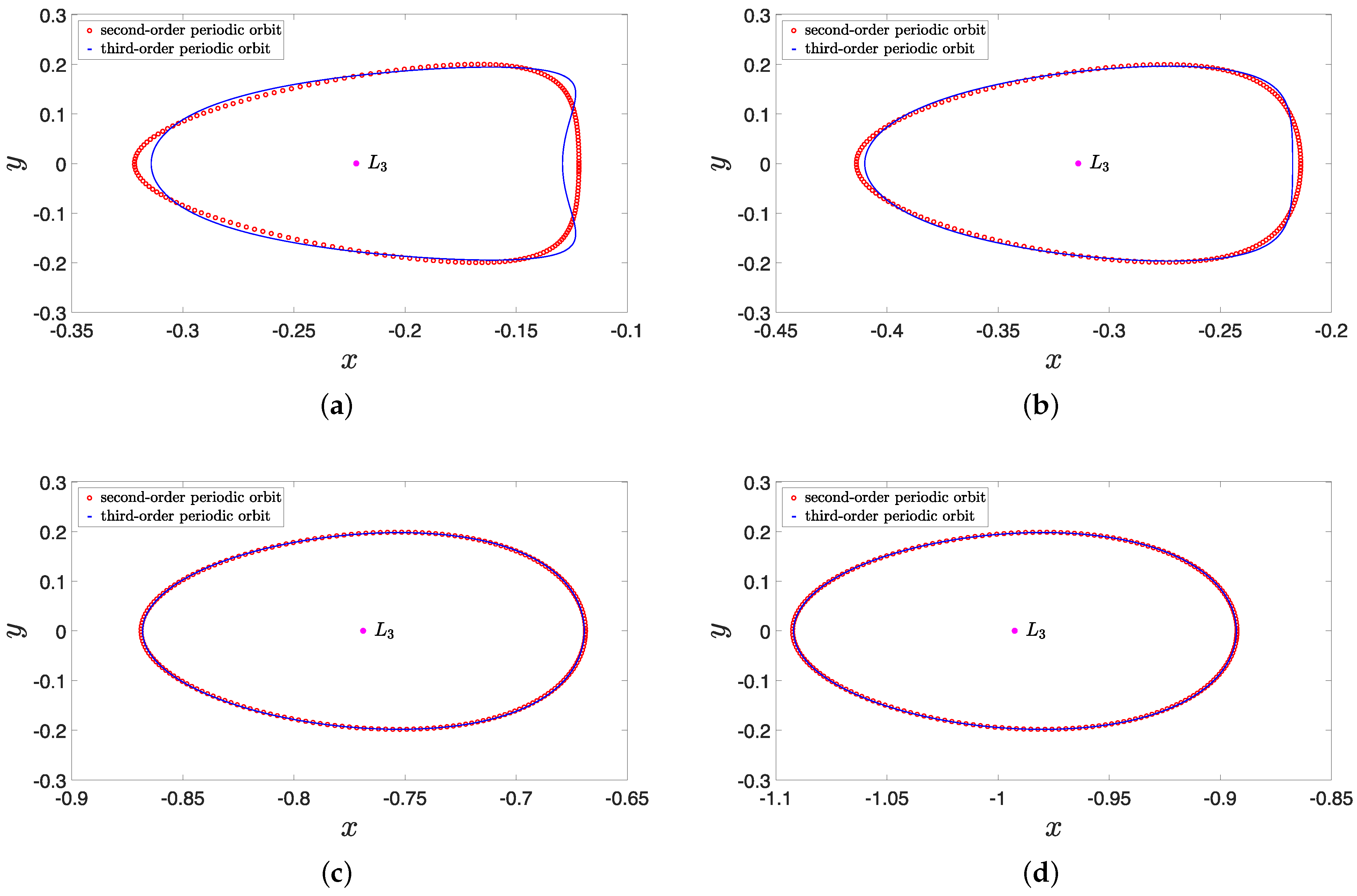
4. Numerical Simulation

This section discusses the influence of the scale parameter $\sigma$ of the regular moons’ mass distribution, the three-body interaction parameter k, and the variable-mass parameter $\gamma$ on the dynamic behavior of the periodic orbit near the Lagrangian point $L_3$. According to Stefan–Boltzmann’s theorem [35], the radiation factor parameters of the Sun and Saturn are $q_1\approx q_2\approx 1$. In addition, the actual mass ratio parameter of the Sun and Saturn is $\mu =0.0002857$.

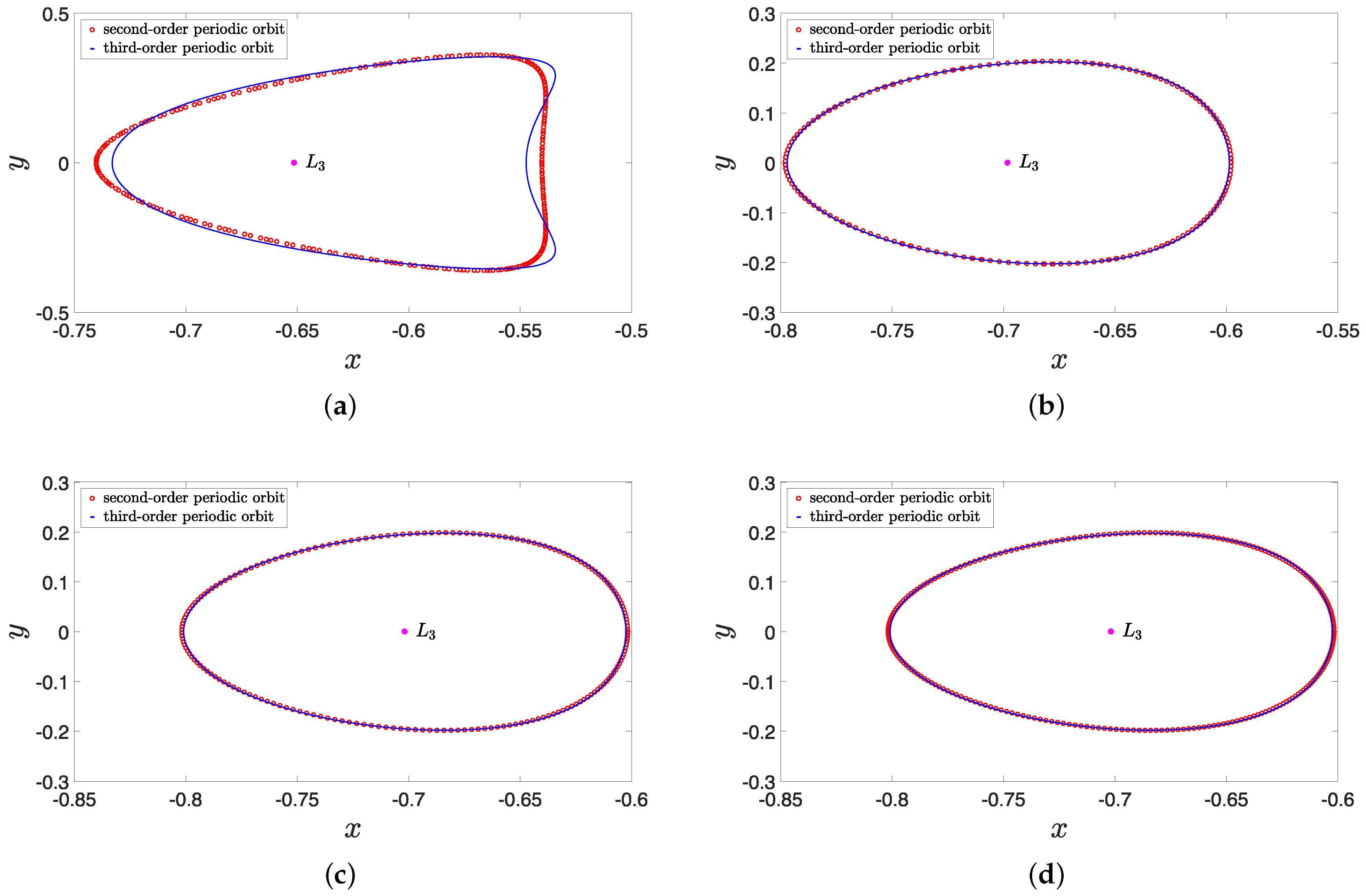
4.1. Influence of the Scale Parameter $\sigma$

According to the value range of parameter k in [23], we chose $k=-0.03$, and $\gamma =0.5$, $\epsilon =0.1$. When the scale parameter $\sigma$ of the lognormal distribution is 1, 2, 7.82406, and 100, the second- and third-order approximate periodic orbits near the Lagrangian point $L_3$ on the x-y plane are shown in Figure 2. The degree of agreement between the second-order and third-order approximate periodic orbits increases as $\sigma$ increases. To visualize the influence of the change in the value of $\sigma$ on the periodic orbit, we depict the third-order periodic orbits corresponding to different values of $\sigma$ in the same three-dimensional coordinate system and project them to the three coordinate axis planes, as shown in Figure 3.

When the scale parameter $\sigma$ located on the denominator of the potential energy function decreases, we found that the shape of the periodic orbits becomes complicated, as shown in Figure 2 and Figure 3. With the increase in $\sigma$ in Figure 3, the shape of the third-order approximate periodic orbit hardly changes, the position of Lagrangian point $L_3$ gradually moves away from the center-of-mass and then stays near $(-0.7018,0)$, and the periodic orbit in the directions of x and y finally stabilizes in the area of $(-0.8,-0.6)\times (-0.2,0.2)$. The range of $\sigma$ is limited to the confidence interval $[6.05109,11.0738]$. In this case, we found that not only the second- and third-order periodic orbits are very close to each other under a given $\sigma$-value in the confidence interval, but also the shape and amplitude of the orbit, and the position of the Lagrangian point $L_3$ remains almost unchanged. This also indicates that when the moons’ mass obeys the best-fitting distribution, the statistical error has a minimal effect on the periodic orbit near the Lagrangian point $L_3$.

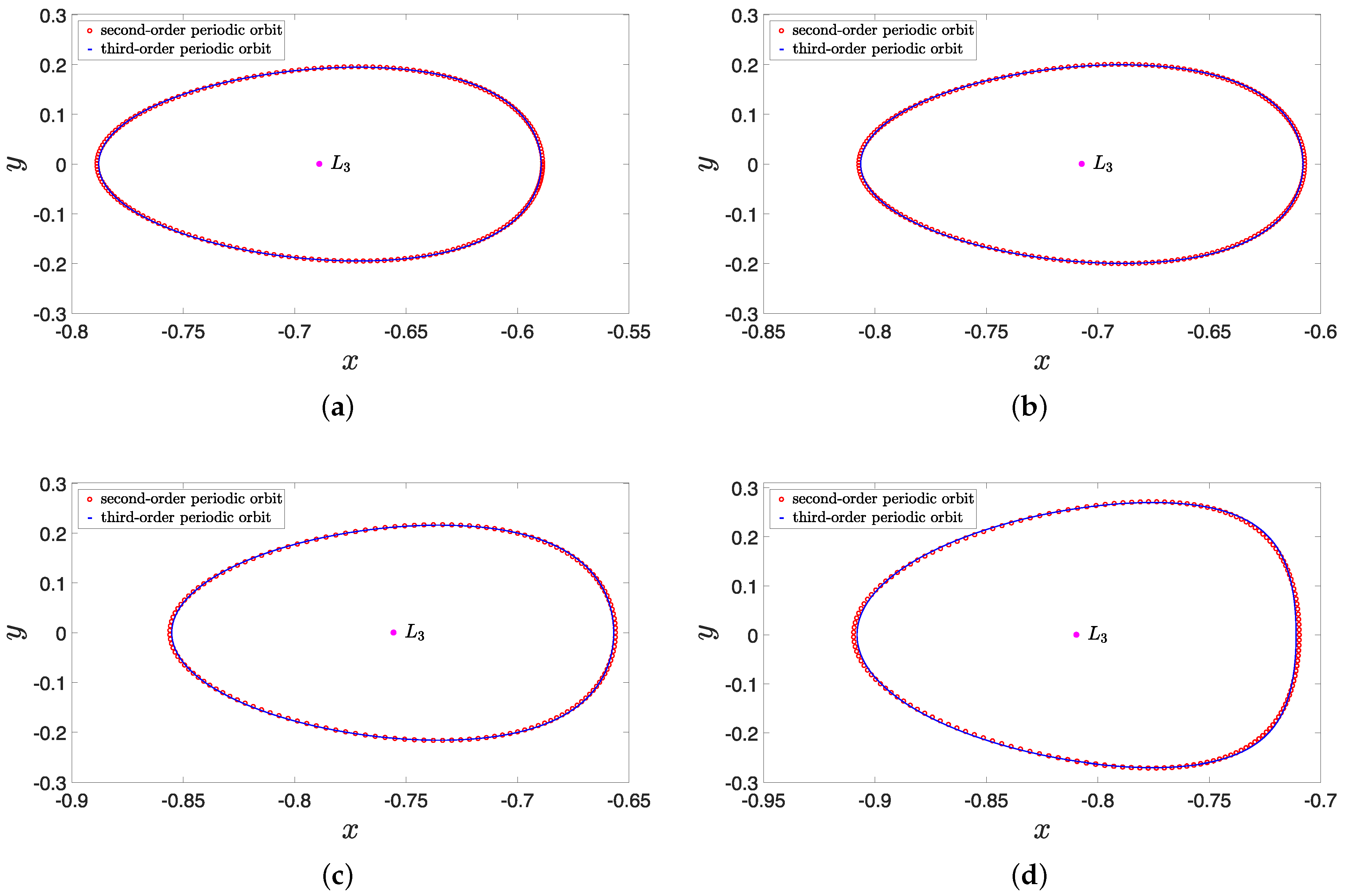
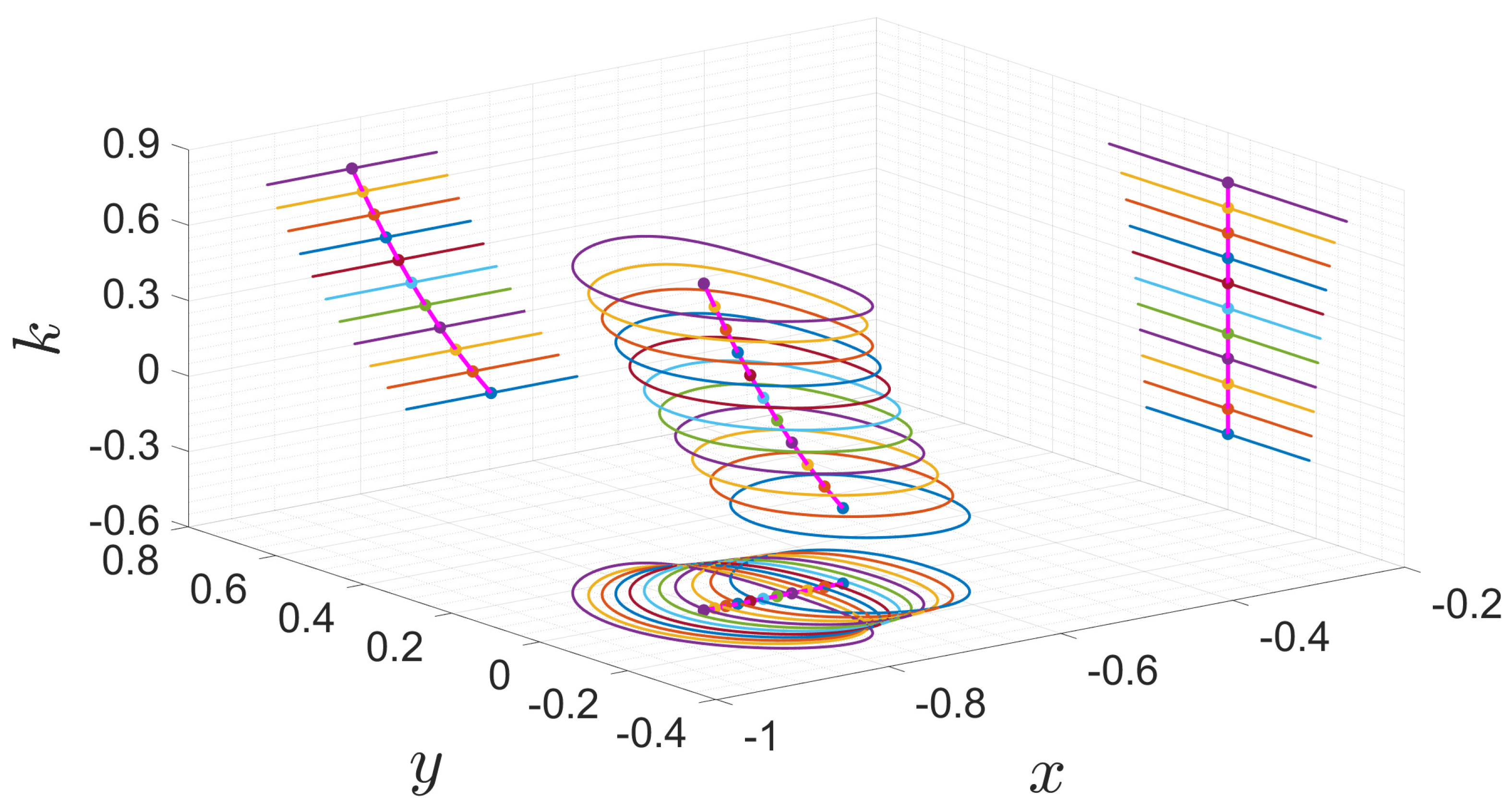
4.2. Influence of the Three-Body Interaction Parameter k

We selected the parameters $\gamma =0.5$, $\sigma =0.65$, and $\epsilon =0.1$. The approximate periodic orbits near the Lagrangian point $L_3$ on the x-y plane are shown in Figure 4 when k takes −0.1, 0, 0.3, and 0.7.

To examine the influence of the change in k on the periodic orbit and the position of the Lagrangian point $L_3$, we describe the third-order periodic orbits corresponding to different values of k in the same three-dimensional coordinate system and projected them to the three coordinate axis planes, as shown in Figure 5.

From Figure 4 and Figure 5, we found that the shapes of the second- and third-order periodic orbits have slight differences when k takes a given value. At this time, the degree of agreement between approximate periodic orbits of different orders cannot be effectively improved by increasing the orbital order. Moreover, as shown in the projections of Figure 5, the periodic orbit amplitudes along the x-direction do not change with the increasing k, but they gradually increase along the y-direction. In addition, the periodic orbits and the position of the Lagrangian point $L_3$ move away from the center-of-mass.

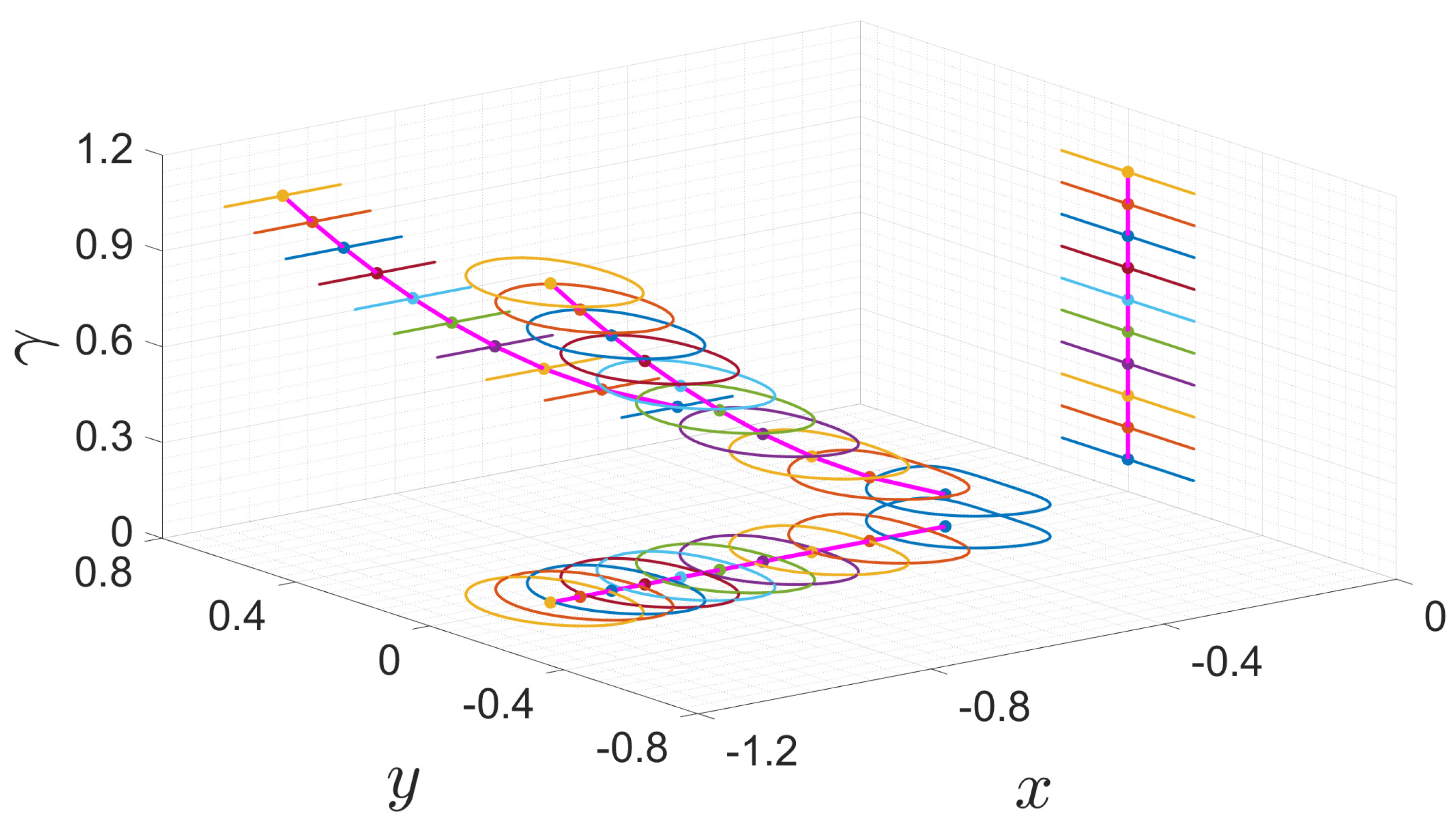
4.3. Influence of the Variable-Mass Parameter $\gamma$

W selected the parameters $\sigma =0.65$, $k=-0.03$, and $\epsilon =0.1$. The approximate periodic orbits near the Lagrangian point $L_3$ on the x-y plane are shown in Figure 6, when the variable-mass parameter $\gamma$ ($0\le \gamma \le 1$) of the third body is 0.05, 0.1, 0.6, and 1.

Similarly, to explore the influence of the variable-mass parameter $\gamma$ on the periodic orbits and the position of the Lagrangian point $L_3$, we describe the third-order periodic orbits corresponding to different values of $\gamma$ in the same three-dimensional coordinate system and projected them onto the three coordinate axis planes, as shown in Figure 7.

Figure 6 and Figure 7 show that the difference between the second- and third-order approximate periodic orbits is considerable when $\gamma$ is small. This is because a smaller $\gamma$ corresponds to a smaller third-body mass; in addition to being affected by the gravitational force of the Sun and Saturn, it is also vulnerable to the gravitational or perturbation factors of other celestial bodies, resulting in poor orbital stability, and there is an apparent difference between orbits of different orders. When $\gamma$ is close to one, the degree of agreement between the second- and third-order periodic orbits is near perfect, and the second-order periodic orbit can be used to approximately replace the third-order periodic orbit. As the mass of the third body decreases, that is as $\gamma$ decreases, the periodic orbit will shift towards the center-of-mass, and the position of the Lagrangian point $L_3$ will gradually approach the center-of-mass of the system. However, the change in $\gamma$ hardly affects the amplitude of the periodic orbit, and the areas of the periodic orbits are also approximately equal.

5. Conclusions

Based on the nonparametric test in statistics, this paper concluded that the best distribution of the mass of Saturn’s regular moons is the lognormal distribution. A p-value close to one indicates that the best-fitting works well. According to the results of statistical inference, a mass function relationship that is different from the empirical Jeans’ law was obtained, and on this basis, the dynamic equations of the variable mass restricted three-body problem were established. With the help of the Lindstedt–Poincaré perturbation method, the analytical expression of the approximate periodic orbit near the Lagrangian point $L_3$ was obtained. In addition, the effects of changes in scale parameter $\sigma$, the three-body interaction parameter k, and the variable-mass parameter $\gamma$ on the periodic orbit and the position of the Lagrangian point $L_3$ were also discussed.

When $\sigma$ increases, the Lagrangian point $L_3$ will gradually move away from the system’s center-of-mass, and the degree of coincidence between the second- and third-order periodic orbits will also be significantly improved. In the range of its confidence interval $[6.05109,11.0738]$, the shape and amplitude of the orbit and the position of the Lagrangian point $L_3$ will remain almost unchanged, which shows that the statistical error has a small effect on the periodic orbit near the Lagrangian point $L_3$. For the change of k, the difference between the second- and third-order periodic orbits will not change significantly, but the increase of the value of k will not only make the Lagrangian point $L_3$ move back to the center-of-mass of the system, but also, the amplitude of the orbit will increase. The closer $\gamma$ is to one, the better the coincidence between the second- and third-order periodic orbits. In the mission of orbit design, it is believed that the second-order periodic orbit can replace the third-order periodic orbit as the initial approximation of the orbit design. Within a specific range, the change in $\gamma$ will only affect the evolution of the periodic orbit and the Lagrangian point $L_3$.

References

1. Sheppard, S.S. New Saturn Moons. Available online: https://sites.google.com/carnegiescience.edu/sheppard/home/newsaturnmoons2019 (accessed on 8 October 2021).
2. Sheppard, S.S. Saturn Moons. Available online: https://sites.google.com/carnegiescience.edu/sheppard/moons/saturnmoons (accessed on 8 October 2021).
3. Dones, L.; Chapman, C.R.; McKinnon, W.B.; Melosh, H.J.; Kirchoff, M.R.; Neukum, G.; Zahnle, K.J. Icy satellites of Saturn: Impact cratering and age determination. In Saturn from Cassini-Huygens; Springer: Dordrecht, The Netherlands, 2009. [Google Scholar]
4. Hirata, N. Differential impact cratering of Saturn’s satellites by heliocentric impactors. J. Geophys. Res. Planets 2016, 121, 111–117. [Google Scholar] [CrossRef] [Green Version]
5. Dorofeeva, V.A. Genesis of volatile components at Saturn’s regular satellites. Origin of Titan’s atmosphere. Geochem. Int. 2016, 54, 7–26. [Google Scholar] [CrossRef]
6. Castillo-Rogez, J.; Vernazza, P.; Walsh, K. Geophysical evidence that Saturn’s moon Phoebe originated from a C-type asteroid reservoir. Mon. Not. R. Astron. Soc. 2019, 486, 538–543. [Google Scholar] [CrossRef]
7. Gao, F.B.; Zhu, X.H.; Liu, X.; Wang, R.F. Distribution inference for physical and orbital properties of Jupiter’s moons. Adv. Astron. 2018, 2018, 1894850. [Google Scholar] [CrossRef]
8. Gao, F.B.; Liu, X. Revisiting the distributions of Jupiter’s irregular moons: I. physical characteristics. Bulg. Astron. J. 2021, 34, 113–135. [Google Scholar]
9. Wang, R.F.; Wang, Y.Q.; Gao, F.B. Bifurcation analysis and approximate analytical periodic solution of ER3BP with radiation and albedo effects. Astrophys. Space Sci. 2021, 366, 29. [Google Scholar] [CrossRef]
10. Gao, F.B.; Wang, R.F. Bifurcation analysis and periodic solutions of the HD 191408 system with triaxial and radiative perturbations. Universe 2020, 6, 35. [Google Scholar] [CrossRef] [Green Version]
11. Gao, F.B.; Wang, Y.Q. Approximate analytical periodic solutions to the restricted three-body problem with perturbation, oblateness, radiation and varying mass. Universe 2020, 6, 110. [Google Scholar] [CrossRef]
12. Abouelmagd, E.I.; Selim, H.H.; Minglibayev, M.Z.; Kushekbay, A.K. A new model emerged from the three-body problem within frame of variable mass. Astron. Rep. 2021, 65, 1170–1178. [Google Scholar] [CrossRef]
13. Suraj, M.S.; Aggarwal, R.; Asique, M.C.; Mittal, A. On the modified circular restricted three-body problem with variable mass. New Astron. 2021, 84, 101510. [Google Scholar] [CrossRef]
14. Letelier, P.S.; da Silva, T.A. Solutions to the restricted three-body problem with variable mass. Astrophys. Space Sci. 2011, 332, 325–329. [Google Scholar] [CrossRef] [Green Version]
15. Zhang, M.J.; Zhao, C.Y.; Xiong, Y.Q. On the triangular libration points in photogravitational restricted three-body problem with variable mass. Astrophys. Space Sci. 2012, 337, 107–113. [Google Scholar] [CrossRef]
16. Shrivastava, A.K.; Ishwar, B. Equations of motion of the restricted problem of three bodies with variable mass. Celest. Mech. 1983, 30, 323–328. [Google Scholar] [CrossRef]
17. Ansari, A.A.; Alhussain, Z.A.; Prasad, S.N. Circular restricted three-body problem when both the primaries are heterogeneous spheroid of three layers and infinitesimal body varies its mass. J. Astrophys. Astron. 2018, 39, 1–20. [Google Scholar] [CrossRef]
18. Singh, J. Nonlinear stability of equilibrium points in the restricted three-body problem with variable mass. Astrophys. Space Sci. 2008, 314, 281–289. [Google Scholar] [CrossRef]
19. Singh, J.; Richard, T.K. A study on the positions and velocity sensitivities in the restricted three-body problem with radiating and oblate primaries. New Astron. 2022, 91, 101704. [Google Scholar] [CrossRef]
20. Yang, H.; Bai, X.; Li, S. Artificial equilibrium points near irregular-shaped asteroids with continuous thrust. J. Guid. Control Dyn. 2018, 41, 1308–1319. [Google Scholar] [CrossRef]
21. Ershkov, S.; Leshchenko, D.; Abouelmagd, E.I. About influence of differential rotation in convection zone of gaseous or fluid giant planet (Uranus) onto the parameters of orbits of satellites. Eur. Phys. J. Plus 2021, 136, 1–9. [Google Scholar] [CrossRef]
22. Zotos, E.E.; Chen, W.; Abouelmagd, E.I.; Han, H. Basins of convergence of equilibrium points in the restricted three-body problem with modified gravitational potential. Chaos Solitons Fractals 2020, 134, 109704. [Google Scholar] [CrossRef]
23. Bosanac, N.; Howell, K.C.; Fischbach, E. A natural autonomous force added in the restricted problem and explored via stability analysis and discrete variational mechanics. Astrophys. Space Sci. 2016, 361, 49. [Google Scholar] [CrossRef]
24. Suraj, M.S.; Aggarwal, R.; Asique, M.C.; Mittal, A.; Jain, M.; Paliwal, V.K. Effect of three-body interaction on the topology of basins of convergence linked to the libration points in the R3BP. Planet. Space Sci. 2021, 205, 105281. [Google Scholar] [CrossRef]
25. Abouelmagd, E.I.; Guirao, J.L.G. On the perturbed restricted three-body problem. Appl. Math. Nonlinear Sci. 2016, 1, 123–144. [Google Scholar] [CrossRef] [Green Version]
26. Poddar, A.K.; Sharma, D. Periodic orbits in the restricted problem of three bodies in a three-dimensional coordinate system when the smaller primary is a triaxial rigid body. Appl. Math. Nonlinear Sci. 2021, 6, 429–438. [Google Scholar] [CrossRef]
27. Abouelmagd, E.I.; Alzahrani, F.; Guirao, J.L.G.; Hobiny, A. Periodic orbits around the collinear libration points. J. Nonlinear Sci. Appl. 2016, 9, 1716–1727. [Google Scholar] [CrossRef]
28. Qian, Y.J.; Zhai, G.Q.; Zhang, W. Planar periodic orbit construction around the triangular libration points based on polynomial constraints. Chin. J. Theor. Appl. Mech. 2017, 49, 154. (In Chinese) [Google Scholar]
29. Šuvakov, M.; Dmitrašinović, V. Three classes of Newtonian three-body planar periodic orbits. Phys. Rev. Lett. 2013, 110, 114301. [Google Scholar] [CrossRef] [PubMed] [Green Version]
30. Li, X.M.; Liao, S.J. On the stability of the three classes of Newtonian three-body planar periodic orbits. Sci. China Phys. Mech. Astron. 2014, 57, 2121–2126. [Google Scholar] [CrossRef] [Green Version]
31. Li, X.M.; Jing, Y.P.; Liao, S.J. Over a thousand new periodic orbits of a planar three-body system with unequal masses. Publ. Astron. Soc. Jpn. 2018, 70, 64. [Google Scholar] [CrossRef]
32. Pathak, N.; Elshaboury, S.M. On the triangular points within frame of the restricted three–body problem when both primaries are triaxial rigid bodies. Appl. Math. Nonlinear Sci. 2017, 2, 495–508. [Google Scholar] [CrossRef] [Green Version]
33. Yang, H.; Yan, J.; Li, S. Fast computation of the Jovian-moon three-body flyby map based on artificial neural networks. Acta Astronaut. 2021. [Google Scholar] [CrossRef]
34. Hu, H.Y. Applied Nonlinear Dynamics; China Aeronautical Industry Press: Beijing, China, 2000. (In Chinese) [Google Scholar]
35. Zheng, X.T.; Tu, L.Z. Photogravitationally restricted three-body problem and coplanar libration point. Chin. Phys. Lett. 1993, 10, 61. [Google Scholar] [CrossRef]
Figure 1. The mass CDF of Saturn’s regular moons and the corresponding CDF of the best-fitting distribution.
Universe 08 00063 g001
Figure 2. Approximate periodic orbits near the Lagrangian point L 3 when (a) σ = 1, (b) σ = 2, (c) σ = 7.82406, and (d) σ = 100, respectively.
Universe 08 00063 g002
Figure 3. Third-order periodic orbits and their planar projections under different σ -values.
Universe 08 00063 g003
Figure 4. Approximate periodic orbits near the Lagrangian point L 3 when (a) k = 0.1 , (b) k = 0, (c) k = 0.3, and (d) k = 0.7, respectively.
Universe 08 00063 g004
Figure 5. Third-order periodic orbits and their planar projections under different k -values.
Universe 08 00063 g005
Figure 6. Approximate periodic orbits near the Lagrangian point L 3 when (a) γ = 0.05, (b) γ = 0.1, (c) γ = 0.6, and (d) γ = 1, respectively.
Universe 08 00063 g006
Figure 7. Third-order periodic orbits and their planar projections under different γ -values.
Universe 08 00063 g007