Article

The Contribution of Charged Bosons with Right-Handed Neutrinos to the Muon g − 2 Anomaly in the Twin Higgs Models

1
School of Physics and Microelectronics, Zhengzhou University, Zhengzhou 450001, China
2
National Space Science Center, Chinese Academy of Sciences, Beijing 100190, China
3
University of Chinese Academy of Sciences, Beijing 100140, China
4
Beijing Key Lab of Space Environment Exploration, Beijing 100140, China
*
Authors to whom correspondence should be addressed.
Universe 2022, 8(12), 654; https://doi.org/10.3390/universe8120654
Submission received: 2 November 2022 / Revised: 30 November 2022 / Accepted: 2 December 2022 / Published: 11 December 2022
(This article belongs to the Special Issue Origin of the Flavor Structure in the Standard Model and Beyond)

Abstract

:
We examine the charged boson and right-handed neutrino contribution to the muon g 2 anomaly in twin Higgs models with joint constraints of Higgs global fit data, precision electroweak data, leptonic flavor-changing decay μ e γ , and the mass requirement of heavy-gauge bosons. It comes with the conclusion that some parameters, such as the coupling of charged Higgs to the lepton y μ , the top Yukawa y t , and heavy-gauge boson coupling to the lepton V μ are constrained roughly in the range of 0.12 y μ 0.4 , 0.4 y t 0.9 , and 0.47 V μ 1 , respectively.
PACS:
12.60.-i; 12.60.Fr; 14.60.Ef

1. Introduction

The long-standing puzzle of the muon anomalous magnetic moment a μ ( g 2 ) μ / 2 was measured by the E989 muon g 2 anomaly experiment in Fermilab (FNAL) [1] and the Brookheaven National Laboratory (BNL) [2,3],
a μ FNAL + BNL = ( 11659206.1 ± 4.1 ) × 10 10
which has a 4.2 σ deviation from the prediction of the SM [1,4,5]
Δ a μ FNAL + BNL = ( 25.1 ± 5.9 ) × 10 10 .
It may hint at the existence of a new physics beyond the SM. The difference between the experimental data and the SM prediction determines that there is room for new physics. Various new physics scenarios try to explain the muon g 2 excess. For recent works, see, e.g., refs. [6,7,8,9,10,11,12].
So-called twin Higgs (TH) models can be realized by extending the SM with discrete twin symmetry [13] and are quite appealing. First, the discrete symmetry in them connects SM fields with extended ones. Second, more importantly, the extended fields are uncharged under SM gauge groups, i.e., they will appear as singlets, and “show” in upcoming experiments purely as missing energy, escaping from the current constraints of the LHC to new particles [14].
In TH models, the extra charged gauge bosons and charged scalars [15,16] may have leptonic and the quark flavor-changing couplings, which will contribute to a muon anomalous magnetic moment. Since there is not any signal of the twin top and twin gauge bosons in the experiments, their masses may be very heavy, and the phenomenological signatures are suppressed. Therefore, the main contribution to the muon anomaly comes not from heavy twin top and twin gauge bosons, but from the charged Higgs via its Yukawa couplings to SM quarks and leptons.
However, TH models have encountered difficulties in cosmological considerations. In the simplest realization of TH [13] models, the twin particles will eventually transfer their entropies into those of SM photons and neutrinos, which results in deviations from the observations [17,18], greatly increasing the value of N e f f , which is the effective number of (light) neutrino species [19,20].
Various modifications are proposed to reduce the N e f f value in TH models. See, e.g., refs. [20,21,22,23,24,25,26,27]. Type I seesaw [28,29,30,31] is one of the mechanisms to provide tiny neutrino masses by involving the exchange of right-handed neutrinos, and is also one to lower the effective degrees of freedom contributed by the twin sector when it is embedded into TH models [23]. Typical lepton flavor-changing couplings will appear via this mechanism, leading to interesting phenomenological consequences.
Flavor-changing couplings can contribute to the muon anomalous magnetic moment not only at the one-loop level, but also via the two-loop diagrams. Since the quarks are much heavier than the leptons, the phase space suppression may be surpassed by the mass enhancement. Therefore, the two-loop Barr–Zee diagrams [32] may contribute much more largely than that from the one-loop ones, if only the Higgs bosons are not too light [33,34]. Thus, in the following, we will calculate the contributions from both the one-loop and two-loop levels. We will examine the relevant parameter space of TH models by considering the joint effects from the theory, the precision electroweak data, the 125 GeV Higgs signal data and the muon g 2 anomaly.
This paper is organized as follows. In Section 2, we simply present TH models and the relevant couplings. In Section 3, we discuss the rough constraints of the relevant parameters in TH models. In Section 4, we calculate the muon anomalous magnetic moment g 2 at the one-loop level. The analytic expressions for the two-loop muon g 2 anomaly and the Higgs global fit are given in Section 5. In Section 6, we calculate the contributions of the Barr–Zee diagrams and the total constraints. Finally, the conclusion is drawn in Section 7.

2. The TH Models and the Relevant Couplings

The hierarchy problem [35,36,37], which is induced by the disparity between the electroweak scale and the Planck scale, is one of the most outstanding problems in particle physics (see, e.g., [38]). Both supersymmetry [39] and the compositeness of the Higgs [40,41], even the strong breaking models [42,43,44,45,46,47,48,49], where the electroweak scale originates from a supersymmetry breaking scale or a composite scale, or even abandoning the idea of the Higgs as the origin of the electroweak symmetry breaking, have attempted to address the issue.
However, in the new physics models mentioned above, the solutions to the hierarchy problem generically contain the top quark partners that have SM-colored charge with the mass at the electroweak scale. Such particles have very rich phenomenological possibilities, which are easily found at the Large Hadron Collider (LHC). However, so far, there is not any signal of this kind of particle, which constrains their masses severely: typically, larger than 1 TeV [19,50,51,52,53]. To satisfy the bounds of this kind, the parameters in these theories need to be fine-tuned to fix the electroweak scale.
One solution to the above problem is to assume that the Higgs mass is protected by a Z 2 discrete symmetry that copies the SM particles. Therefore, the new particles associated with this symmetry do not have the SM color charge, which is called the twin Higgs (TH) model [13]. This situation makes the new particle states much more difficult to produce and detect at the LHC.
In the original TH framework, the SM particles and their copies are related to discrete Z 2 twin symmetry. To contain a residual custodial symmetry, the global symmetry of the Higgs sector in the simplest realization can be taken as S O ( 8 ) or S O ( 7 ) [15,16,54,55]. The SM Higgs doublet is a part of the pseudo-Nambu–Goldstone boson (pNGB), which arises from the spontaneous breaking of the global S O ( 8 ) ( S O ( 7 ) ) symmetry into S O ( 7 ) ( G 2 ). The neutral Higgs mass, under the joint action of global symmetry and discrete twin symmetry, is protected from one-loop quadratic divergence.
This mechanism can stabilize the Higgs mass up to the energy scale at the order of 5–10 TeV, and solve the so-called “little hierarchy” problem [14]. A lot of models of this kind [13,56,57,58,59,60,61,62,63,64], have been proposed. TH [13] realization is one of the best-known examples. After the twin Higgs obtains a vacuum expectation value f, the SM Higgs has appeared as a pseudo-Nambu–Goldstone (pNG) boson, preventing the Higgs mass from quantum corrections up to the scale Λ T H 4 π f because of the twin symmetry between the top and the colorless top partner.
Ref [13] gives the Higgs contributed by the new gauge bosons and extra fermions and estimates the fine tunings. For example, the contribution of the top partners to the Higgs potential is given as
m h 2 = 3 8 π 2 y 2 M 2 M 2 y 2 f 2 M 2 l n m T A 2 m T B 2 y 2 f 2 l n m m T A 2 2 m t B 2 ,
where y is Yukawa coupling, y H Q L T R + h . c . , and m T A 2 = M 2 + y 2 f 2 , m T B 2 = M 2 , m t B 2 = y 2 f 2 . The reference finally suggests that, for the limit M Λ , with f = 800 GeV, Λ 4 π f 10 TeV, from Equation (3), the Higgs mass is 166 GeV and the fine tuning is 11 % (1 in 9), which is acceptable. The Higgs mass is 153 GeV and the fine tuning is 31 % (1 in 3) for f = 500 GeV, Λ 6 TeV. Therefore, for scale up to the order of 5–10 TeV, the pseudo-Goldstone Higgs mass will be protected against radiative corrections, and one can refer to the original paper [13] for details.

2.1. The Charged Higgses and the Yukawa Couplings to the Third Generation in Twin Higgs Models

Since the minimal coset U ( 4 ) / U ( 3 ) does not contain a residual custodial symmetry, and in the non-linear case the twin mechanism is not realized in the gauge sector within this global group, while S O ( 8 ) / S O ( 7 ) prevents a large custodial breaking in composite models of the twin mechanism, the global symmetry-breaking pattern of the simplest original TH model can be S O ( 8 ) / S O ( 7 ) or S O ( 7 ) / G 2 [15,16,54,55]. Therefore, there are 7 pNGBs after the breaking and 6 of them are eaten by the ordinary and twin gauge bosons, meaning that there will be only one neutral scalar left.
Besides the SM-like neutral Higgs, there would be charged Higgses. Some TH models introduce extra scalars for different goals. For example, to provide suitable neutrino masses via couplings to the right-handed neutrinos, a S U ( 2 ) L singlet charged scalar S + was introduced in [65], while [24,25] add a new scalar ϕ to have a similar effect in couplings with leptons.
Extra charged scalars may also appear in the particle list due to the enlarging breaking mode. The aim of the economical breaking choices mentioned above is to keep breaking smallest, but it can be otherwise. For example, it can be S O ( 8 ) G 2 or S O ( 2 N ) S O ( N ) × S O ( N ) [66] (the former N is for the SM sector and the latter for the twin sector).
In the following, we assume the global breaking is S O ( 8 ) G 2 as an example. After the six gauge bosons obtain masses, the left eight PNGBs can be written as Π matrix
Π = 2 π a ^ T a ^ , a ^ = 1 , , 7 ,
where T a ^ are the broken generators, defined as
T i j a ^ = i 2 t i j a ^ 8 , a ^ = 1 , , 7 .
Here, t i j a b = δ i a δ j b δ j a δ i b , and π a ^ are the Goldstone fields.
Therefore, the 8 scalar degrees of freedom may be packaged into an 8 of S O ( 8 )
ϕ = exp i Π f .
The first 4 components would comprise the Higgs multiplet, and the latter N the twin Higgs. They can also be parameterized via the decomposition 8 = ( 2 , 1 , 2 ) + ( 1 , 2 , 2 ) under S U ( 2 ) L × S U ( 2 ) L ˜ × S U ( 2 ) R ^ as
( 2 , 1 , 2 ) : H = f 2 π 2 + i π 1 π 4 i π 3 , ( 1 , 2 , 2 ) : H ˜ = f 2 π 6 + i π 5 σ i π 7 ,
where f 2 ( π 2 + i π 1 ) can identified as the charged scalar H ± . In some situations, ω ˜ ± f ( π 6 ± i π 5 ) / 2 and ω ˜ 0 f π 7 can also be taken as the long-lived particles.
At low energies, the representations of SO(8) of the third-generation quarks q L and q ˜ L can be written as
Q L = v b b L + v t t L = 1 2 i b L b L i t L t L 0 0 0 0 T , Q ˜ L = v ˜ b b ˜ L + v ˜ t t ˜ L = 1 2 0 0 0 0 i b ˜ L b ˜ L i t ˜ L t ˜ L T ,
while those of t R and t ˜ R are singlets. Thus, the top Yukawa couplings are written as
y t f t ¯ R Σ Q L + y ˜ t f t ˜ ¯ R Σ Q ˜ L + h . c . = y t q ¯ L H t R y ˜ t t ˜ ¯ R H ˜ q ˜ L + h . c . + . . . ,
where q L = ( b , t ) , q ˜ L = ( b ˜ , t ˜ ) .
A Z 2 symmetry q L , t R q ˜ L , t ˜ R leads to y t = y ˜ t . The masses of the rest of the fermions (including twin fermions) are obtained in a similar manner. Due to y ˜ ψ y t , the associated contribution to the Higgs potential of the light fermions will be negligible. Therefore, it is not necessary to enforce the approximate equality y ψ = y ˜ ψ .

2.2. Flavor-Changing Couplings of Leptons in TH Models

In the seesaw type I model [28,29,30,31], to realize the seesaw mechanism, right-handed neutrinos are introduced, and they are singlets under the SM gauge group S U ( 3 ) C × S U ( 2 ) L × U ( 1 ) Y [67]. We denote ν i s as the ordinary tiny neutrinos, and ν i R s as the heavy right-handed neutrinos. The masses of the neutrinos can be described by the following Lagrangian terms
L Y j ν ¯ R H + p L j y j ν ¯ H + p L j + h . c . + . . . ,
In the mass eigenstate basis, the gauge interactions with ν R are given by [68,69],
L g 2 l ¯ j L γ μ V P M N S ν i L W μ + l ¯ j L γ μ V l ν ( ν i R ) L N W μ + h . c . V j ν ¯ R W μ + γ μ P L j + h . c . + . . .
Please note that in the second lines of Equations (10) and (11) and following calculation, we assume that the right-handed neutrinos are degenerate, i.e., ν 1 R = ν 2 R = ν 3 R = ν R , which means that there is only one flavor of the heavy neutrino (the same case for the ordinary neutrinos). Therefore, the couplings will be simply written as V j , Y j and y j , respectively, where j can be e, μ , and τ .
Please note that the 3 × 3 Maki–Nakagawa–Sakata (MNS) matrix U M N S [70,71] elements in the above flavor-changing couplings are also absorbed into the couplings and their effects are actually neglected.

3. The Rough Ranges of the Relevant Parameters in TH Models

In this paper, we take the light CP-even Higgs h as the SM-like Higgs, m h = 125.5 GeV. The mass difference between the charged Higgs boson and the neutral heavy Higgs boson should be less than 300 GeV, i.e., | m H ± m 0 | 300 GeV, and in general, the mass of the neutral heavy Higgs boson is larger than that of the SM-like Higgs [72,73]. We here, however, just roughly scan over the charged Higgs mass m H ± in the following ranges:
100 GeV < m H ± < 1000 GeV .
In the following, we will simply discuss the constraints on the parameters:
(1)
The first constraint comes from the signal data of the 125 GeV Higgs, which is important, since the couplings of the SM-like Higgs with the fermions and the bosons in TH models can deviate from the SM largely and the production and decay modes of the SM-like Higgs may be modified severely. In the paper, we will perform the calculation of χ h 2 for the signal strengths of the 125 GeV Higgs, which will be shown in Section 5 and Section 6.
(2)
The constraints on parameter f come from the joint effects of the Z-pole precision measurements, the low-energy neutral current process, and the high-energy precision measurements off the Z-pole indirectly, and according to all these data, f should be larger than 500–600 GeV [74]. On the other hand, to control in a mild fine tuning, f should not be too large, since the fine tuning is more severe for large f. The constraints for f can also come from the flavor-changing decay μ e γ : With the experimental constraints, [75,76], BR ( μ e γ ) < 4.2 × 10 13 , the flavor-changing decay μ e γ will give f [ 0.6 2 ] TeV.
So after we take the above constraints from the electroweak precision measurements and the LHC data into account, we can assume that 500 f 2000 GeV. In our numerical evaluations, however, we have not taken f as a free parameter. Instead, we assume the characteristic mass and coupling of the composite resonances is set by m and g, respectively, which are related by the symmetry-breaking order parameter, f, as m = g f .
(3)
In the present experiments, m W H ± has been constrained stringently [77,78,79]. The ATLAS experiment has presented the first search for dilepton resonances based on the full Run 2 data-set [77,79] and set limits on the W production cross-section times branching fraction in the process
σ ( p p W X ) × B R ( W ν )
for M W in the 0.15 TeV–7 TeV range, correspondingly. Recently, similar searches have also been presented by the CMS Collaboration using 140 fb 1 of data recorded at s = 13 TeV [78]. The most stringent limits on the mass of W boson to date come from the searches in the above process by the ATLAS and CMS collaborations using data taken at s = 13 TeV in Run 2 and set a 95% confidence level (CL) lower limit on the W mass of 6.0 TeV [79].
This analysis, however, is based on the simplest models [80] such as the sequential standard model proposed by Altarelli et al. [81], which is usually taken as a convenient benchmark in the experiments. In the simplest models, the gauge particles are considered to be the copies of the SM gauge bosons, and their couplings to fermions are in the same mode as those of the SM gauge bosons, but they miss trilinear couplings such as W W Z and Z W W , etc. Therefore, the situation that the sequential standard model [81] has acted as a reference for experimental extended gauge boson searches may be changed, and the results may be re-interpreted in the context of other new physics models [82]. In the following computation, we will check the sensitivity of the charged heavy-gauge boson with the mass range 1 m W H ± 20 TeV.
(4)
Regarding the top Yukawa y t , at the EW scale, it should be the same as that in the SM, but at the higher scale, each will be different. Since in general, we assume that the top quark is connected to electroweak symmetry breaking and sensitive to new physics models, we scan the top Yukawa y t from zero to 1.5 times of the SM top Yukawa y t S M . The heavy-gauge boson couplings to the lepton V μ is also from zero to 1.5 times of the SM couplings V μ S M .
From the relationship of the masses of the ordinary neutrino and the right-handed neutrino, m ν Y μ 2 v 2 m ν R [20], we can estimate the Yukawa coupling Y μ is roughly 10 5 10 3 when the right-handed neutrino masses are taken in the order of TeV and the ordinary neutrino masses are assumed as 10 3 10 1 eV. Or, if the right-handed mass m ν R is free, this relationship may serve as a constraint on Y μ .

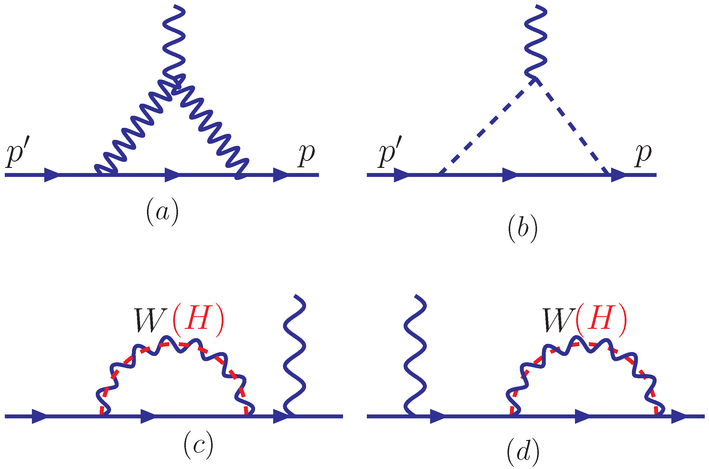
4. The One-Loop Muon Anomalous Magnetic Moment g 2

From the couplings of Equations (10) and (11), one can easily calculate the new contributions to the muon anomalous magnetic moment, which are generated by one-loop diagrams involving the exchange of W μ gauge boson and charged scalar H ± with heavy neutrino, as shown in Figure 1.
Please note that the contributions from Figure 1c,d contain self-energy of the fermions, which is proportional to γ λ , and they do not contribute to the muon anomalous moment. That is because, when the Lorentz structure is written as the matrix element of the electromagnetic current between incoming and outgoing fermion states of momentum and spin { p , s } and { p , s } , respectively,
< p , s | J λ e m | p , s > = μ ¯ e ( p , s ) { F 1 ( Q 2 ) γ λ + F 2 ( Q 2 ) 2 m · i 2 [ γ λ , γ ν ] · q ν } μ p ( p , s ) ,
the second term, F 2 ( 0 ) = g 2 2 a μ ( Q = p p ), while the first term, i.e., Figure 1c,d does not contribute the muon anomalous magnetic moment.
The one-loop contribution to the muon anomalous magnetic moment can be written as [83,84,85]:
Δ a μ T H = Δ a μ ν R W + Δ a μ ν R H + Δ a μ ν H + Δ a μ ν W H .
Δ a μ . R W ( 1 loop ) = V μ 2 m μ 2 8 π 2 0 1 d x x 2 ( 1 + x ) x ( 1 x ) m ν R 2 m W 2 m W 2 x + m ν R 2 ( 1 x ) ,
Δ a μ . W H ( 1 loop ) = g 2 2 m μ 2 8 π 2 0 1 d x x 2 ( 1 + x ) m W H 2 x + m ν 2 ( 1 x ) ,
Δ a μ . R H ( 1 loop ) = Y μ 2 m μ 2 16 π 2 0 1 d x x 3 x 2 m H 2 x + m ν R 2 ( 1 x ) ,
Δ a μ . H ( 1 loop ) = y μ 2 m μ 2 16 π 2 0 1 d x x 3 x 2 m H 2 x + m ν 2 ( 1 x ) ,
where g 2 is the W ( W H ) boson couplings to the leptons, similar to that in the SM.
Figure 2 shows that the contributions of the charged Higgs, the heavy charged bosons and the heavy neutrino at one-loop level, and we find that the contributions from ν W H , ν H ± loop are quite small, about ∼ 10 11 , which cannot explain the discrepancy between the experiments and the theoretical prediction. Due to the heavy neutrino mass suppression, the ν R H ± loop is even smaller, about 10 31 , which is too small and does not show in Figure 2.
When m ν R is very small, the ν R W loop contribution given as Equation (16) is large, just as that in [7,86], Δ a μ . R W approximatively equals to the one-loop contribution predicted by the SM, Δ a μ . R W 10 9 . Please note that the contribution is positive. However, in our case, m ν R Y μ 2 v 2 / m ν m W , from Equation (16), the ν R W contribution can be approximately given as V μ 2 m μ 2 16 π 2 m W 2 10 9 , which is negative and widens the discrepancy between theory and experiment. This further constrains the mixing matrix element V μ , which will have to be significantly suppressed. Therefore, in our parameter space, the total contribution of the one-loop contribution is negative, which makes it impossible to arrive at the required order of the experiments.
Therefore, we can conclude that in the twin Higgs models, the one-loop contribution cannot remedy the discrepancy between the experiments and the theoretical calculation. Since in the two-loop Barr–Zee contribution, the large mass ratio of quarks to leptons may surpass the phase suppression compared to that at the one-loop level, and perhaps more parameters contribute to the muon anomalous magnetic moment, it will be of importance to consider the two-loop level calculation.

5. The Analytic Expressions for the Two-Loop Muon g 2 Anomaly and the 125 GeV Higgs Global Fit in TH Models

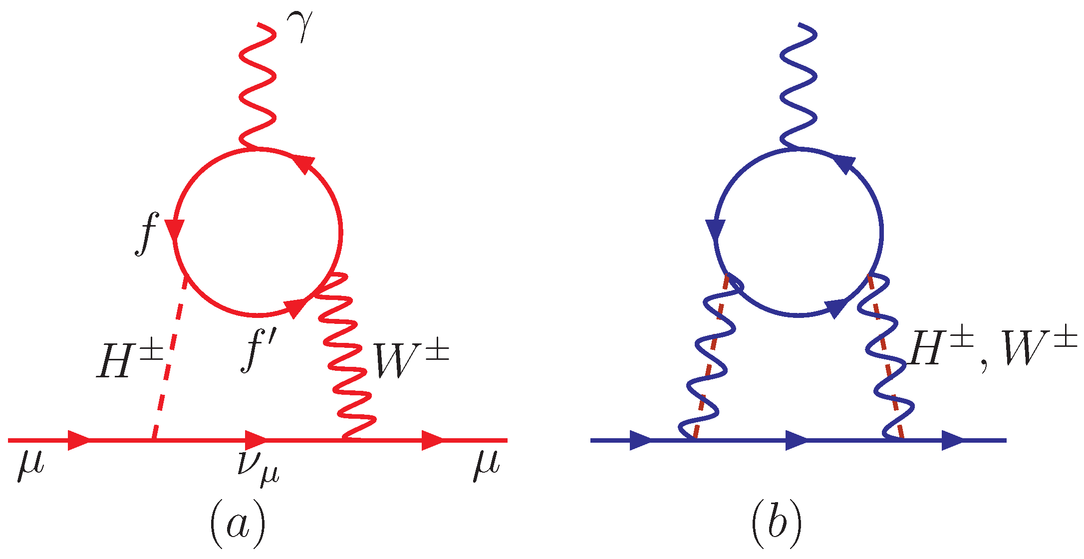
5.1. The Analytic Expressions for Two-Loop Barr–Zee Muon g 2

In TH models, the two-loop Barr–Zee muon g 2 anomaly contributions are mediated by the charged Higgs H ± and the gauge boson with the fermions. The large enhancement factor m q 2 / m μ 2 may surpass the loop suppression phase space factor α / π ; therefore, the two-loop contributions could be more important than one-loop ones. Since the couplings H 0 μ μ ¯ , proportional to m μ / v , is too small to have large contribution in the two-loop diagrams, and due to the discrete symmetry, it is usually difficult to form couplings such as W Z H + , W γ H + , W h 0 H + etc., [87], and the heavy-gauge boson mass suppression, we will just consider the diagrams given in Figure 3.
Please note that, in the Barr–Zee two-loop diagrams, there are no two scalars or two W ± charged bosons connect to the triangle loop simultaneously due to the helicity constraints. Since between the two charged particles in the quark loop, the fermion is the bottom quark, the slash momentum terms must vanish undergoing a single γ matrix because of the much smaller mass of the bottom quark compared to the top quark, shown in Figure 3b. Thus, the only contribution comes from Figure 3a.
In Figure 3a, the fermion loop can consist of not only top and bottom quark t t b , b b t , but also the lepton with the right-handed neutrino v R , since the neutrino mass might be quite large. The Barr–Zee two-loop contribution from quark loop can be written as [11,88,89,90,91,92,93,94,95,96,97,98,99,100,101,102,103],
Δ a μ ( t t b + b b t ) = 4 m μ 2 · g V t b 2 · g 2 · 1 512 π 4 N t c m H + 2 m W 2 0 1 d x [ Q t x + Q b ( 1 x ) ] G m t 2 m H + 2 , m b 2 m H + 2 G m t 2 m W 2 , m b 2 m W 2 × Γ t b H + , R * Γ ν μ μ H + m t m μ x ( 1 + x )
where Γ t b H + , R = i y t , Γ ν μ H + = i y μ are the couplings of H + t ¯ b and H + ν ¯ μ , respectively, and P R , L = 1 2 ( 1 ± γ 5 ) . The loop function is defined as,
G ( r a , r b ) = ln r a x + r b ( 1 x ) x ( 1 x ) x ( 1 x ) r a x r b ( 1 x ) .
For the ν R loop when the heavy neutrinos enter the loop, the contribution can be obtained by replacing m t , m b , Q t and Q b by m ν R , m , Q ν R = 0 and Q = 1 , respectively, in Equation (20), which can be written explicitly as
Δ a μ ( ν R ) = 4 m μ 2 · g 2 · V μ · 1 512 π 4 1 m H + 2 m W 2 0 1 d x Q l ( 1 x ) G m ν R 2 m H + 2 , m 2 m H + 2 G m ν R 2 m W 2 , m 2 m W 2 × Γ ν R H + , R * Γ ν μ μ H + m ν R m μ x ( 1 + x )
where Γ ν R H + , R = i Y μ .

5.2. Global Fit of the 125 GeV Higgs

We will perform a global fit to the 125 GeV Higgs signal data and a large number of observables. For the given neutral SM-like scalar-field h and its couplings, the χ h 2 function can be defined as
χ h 2 = k μ k μ ^ k 2 σ k 2 ,
where k runs over the different production(decay) channels considered, and μ k is the corresponding theoretical predictions for the TH parameters. μ ^ k and σ k denote the measured Higgs signal strengths and their one-sigma errors, respectively, and their choices in this work appear in [104,105,106], though the data and the references listed are not complete.
The Higgs signal strengths, employed in the experimental data on Higgs searches, measure the observable cross-sections compared to the corresponding SM predictions. At the LHC, the SM-like Higgs particle is generated by the following production procedures: gluon fusion ( g g H ), vector boson fusion ( q q q q V V q q H ), associated production with a vector boson ( q q ¯ W H / Z H ), and the associated production with a t t ¯ pair ( q q ¯ / g g t t ¯ H ). Meanwhile, the Higgs decay channels are γ γ , Z Z ( * ) , W W ( * ) , b b ¯ and τ + τ . The expressions of the Higgs signal strengths have been shown in [11] and we will not repeat them here.

6. The Calculation of the Barr–Zee Diagrams and the Final Total Constraints from the One- and Two-Loop Contribution

Though in Equations (10) and (11), the LFV couplings are induced by the SM gauge bosons, we here still consider the twin, i.e., heavy-gauge bosons, which have the same LFV couplings, but the heavy-gauge bosons are quite heavier, about 1 TeV or more, just as the discussion above.
In Figure 4, we give the comparison of the contribution at the two-loop level between the inner lines of the SM charged gauge bosons and the TH heavy charged boson and that from the right-handed neutrino loop with the SM charged leptons. The green shadow area in the figure shows the discrepancy between the SM and the measurement for the anomalous magnetic moment Δ a μ .
From Figure 4 we can see the heavy mass of the gauge boson suppressing the contribution, and the contribution is smaller than that of the SM gauge boson, which can be seen from the blue and red curves. We also consider the lepton ν R loop contribution with the charged Higgs and the SM W ± , which is shown via the bottom curve in Figure 4, and it is much smaller than the other contributions. Hence, the total two-loop contribution comes from not only the SM W ± , but also from the heavy W H ± , together with both quark loop and lepton loop, and not the same as those in the one-loop, the contributions are all positive in the parameter spaces under consideration.
Please note that the coupling Y μ is related to the ordinary neutrino masses and the heavy neutrino mass m ν R , just as shown in Section 3 (4), m ν Y μ 2 v 2 m ν R , or m ν R Y μ 2 v 2 m ν . Since the upper bound of the heavy neutrino mass is not provided in the experiments, we here just assume the mass is a parameter determined by the coupling Y μ and the ordinary neutrino mass. With larger couplings and the tiny neutrino mass, the heavy neutrino mass is quite large, so the contribution to the two-loop muon anomalous magnetic moment will be very small due to the mass depression, as shown in Figure 4.
Moreover, from Equation (22) and Figure 4, we know that the contribution from the ν R loop is so small that the only coupling Y μ related to it is not important in determining the g 2 calculation, and at the same time, Y μ has nothing to do with other processes. Therefore, we here take it as a fixed value: Y μ = 0.004 .
However, the contributions in Figure 4 are given for the parameters only varying with the charged Higgs mass and without including one-loop ones. Therefore, in Figure 5, we will show the tendency of the total contribution, including not only at the two-loop but also at the one-loop level, along with the other parameters. From Figure 5 we can see that Δ a μ increases with the increasing couplings y μ and y t but decreases with the increasing V μ , which is because the largest one-loop process to Δ a μ is from ν R W loop with a negative value, and when V μ increases, it will be larger towards the negative direction. Under current parameter conditions, when V μ = 0.7 , the total contribution begins to be positive, and the experiments require V μ in the range of 0.47 V μ 0.66 . For y μ and y t , to arrive at the discrepancy level, relatively large values are required: y μ 0.52 and 0.43 y t 0.65 . From Figure 4 and Figure 5, we can see that the total contribution can arrive at the required range in some parameter spaces.
Next, we scan the anomalous magnetic moment and the Higgs global fit by taking 10,000 random points, so the more the points are left, the higher the possibility of the event is to be probed in the experiments. We restate the parameter ranges: 100 m H ± 1000 GeV, 0 y t 1.5 , 0 V μ 1.2 and 0 y μ 0.5 .
Since χ h 2 fits to the 125 GeV Higgs decay signal data, and we here assume that the neutral Higgs in TH models does not mix with the charged Higgs, the masses of the charged Higgs and the heavy neutrinos contribute little to the Higgs strength χ h 2 , and at the same time, they will hardly be constricted by it, too. On the other hand, due to the quite large top mass, the top Yukawa coupling contributes to the χ h 2 value much more than those from the others. Therefore, in Figure 6, we will show the surviving samples only on the planes of the couplings: y μ V μ , y t y μ and y t V μ , for the Higgs strengthen in the 3 σ confidence level. Figure 6 shows that χ h 2 favors large y t , while it is not sensitive to the other couplings.
In Figure 7, we further impose the two-loop g 2 anomaly constraints on the surviving sample points of χ h 2 within 3 σ possibility on the planes of y t m H ± , y t V μ , V μ y μ , and y t y μ . From the first figure in Figure 7, we can see that the charged Higgs mass is not constrained too much, but the surviving samples favor a larger y t .
We also see from Equation (20) that the g 2 anomaly varies with the top Yukawa coupling y t , so coupling y t should matter a lot, which can be seen from the other figures in Figure 7. This relevance will constrain y t greatly, and it can grossly read as 0.4 y t 0.9 . Another parameter which receives strong constraint is y μ in TH models, and from Equation (20) we know if the quark loops contribute greatly that the g 2 anomaly is also relevant to the parameter y μ and favors a large value of y μ . Therefore, in Figure 7 we give the allowed ranges of both with all the constraints, from which we can grossly obtain 0.12 y μ 0.4 . However, the two-loop g 2 anomaly is not sensitive to the coupling V μ , and it is mainly contributed by a TTB-induced loop, given in Equation (20), which can be seen in Figure 4. Therefore, even with the negative one-loop ν R W -mediated process contribution, the total Δ a μ does not constrain so stringently as that in the second diagram of Figure 5: 0.47 V μ 0.66 . For example, in the the right-upper diagram of Figure 7, V μ can even be larger than 1 in extreme cases.

7. Conclusions

We consider the charged Higgs contribution to the muon g 2 anomaly in TH models with the joint constraints of Higgs global fit data. After imposing various relevant theoretical and experimental constraints, we perform the scan over the parameter space of this model to identify the ranges in favor of the muon g 2 explanation. We find that the muon g 2 anomaly can be explained in TH models in some parameter spaces. The Higgs direct search limits from LHC contribute most largely to all the constraints. With the joint constraints from the 125 GeV Higgs signal data, the precision electroweak data, and the leptonic decay, we find that the muon g 2 anomaly constrains the coupling of charged Higgs to the lepton y μ , the top Yukawa y t , and the heavy-gauge boson coupling to the lepton V μ roughly as 0.12 y μ 0.4 , 0.4 y t 0.9 , and 0.47 V μ 1 .

Author Contributions

Conceptualization, G.-L.L.; methodology, P.Z.; formal analysis, G.-L.L. All authors have read and agreed to the published version of the manuscript.

Funding

This work was supported by the National Natural Science Foundation of China under grant 12075213, by the Fundamental Research Cultivation Fund for Young Teachers of Zhengzhou University (JC202041040) and the Academic Improvement Project of Zhengzhou University.

Data Availability Statement

Not Applicable.

Conflicts of Interest

The authors declare no conflict of interest.

References

  1. Abi, B. et al. [Muon g − 2 Collaboration] Measurement of the positive muon anomalous magnetic moment to 0.46 ppm. Phys. Rev. Lett. 2021, 126, 141801. [Google Scholar] [CrossRef] [PubMed]
  2. Zyla, P. et al. [Particle Data Group Collaboration] Review of Particle Physics. PTEP 2020, 2020, 083C01. [Google Scholar]
  3. Bennett, G.W. et al. [Muon g − 2 Collaboration] Final report of the E821 muon anomalous magnetic moment measurement at BNL. Phys. Rev. D 2006, 73, 072003. [Google Scholar] [CrossRef] [Green Version]
  4. Athron, P.; Balázs, C.; Jacob, D.H.; Kotlarski, W.; Stöckinger, D.; Stöckinger-Kim, H. New physics explanations of aμ in light of the FNAL muon g − 2 measurement. J. High Energy Phys. 2021, 9, 080. [Google Scholar] [CrossRef]
  5. Aoyama, T.; Asmussen, N.; Benayoun, M.; Bijnens, J.; Blum, T.; Bruno, M.; Caprini, I.; Calame, C.M.C.; Cè, M.; Colangelo, G.; et al. The anomalous magnetic moment of the muon in the Standard Model. Phys. Rept. 2020, 887, 1–166. [Google Scholar] [CrossRef]
  6. Miller, J.P.; de Rafael, E.; Roberts, B.L. Muon g − 2: Review of theory and experiment. Rept. Prog. Phys. 2007, 70, 795. [Google Scholar] [CrossRef] [Green Version]
  7. Jegerlehner, F.; Nyffeler, A. The muon g − 2. Phys. Rept. 2009, 477, 1–110. [Google Scholar] [CrossRef] [Green Version]
  8. Lindner, M.; Platscher, M.; Queiroz, F.S. A call for new physics: The muon anomalous magnetic moment and lepton flavor violation. Phys. Rept. 2018, 731, 1–82. [Google Scholar] [CrossRef] [Green Version]
  9. Jegerlehner, F. The Muon g − 2 in Progress. Acta Phys. Polon. B 2018, 49, 1157. [Google Scholar] [CrossRef]
  10. Borsanyi, S.; Fodor, Z.; Guenther, J.N.; Hoelbling, C.; Katz, S.D.; Lellouch, L.; Lippert, T.; Miura, K.; Parato, L.; Szabo, K.K.; et al. Leading hadronic contribution to the muon magnetic moment from lattice QCD. Nature 2021, 593, 51–55. [Google Scholar] [CrossRef]
  11. Liu, G.-L.; Zeng, Q.-G. Muon g − 2 Anomaly confronted with the higgs global data in the Left-Right Twin Higgs Models. Eur. Phys. J. C 2019, 79, 612. [Google Scholar] [CrossRef]
  12. Li, Z.; Liu, G.-L.; Wang, F.; Yang, J.M.; Zhang, Y. Gluino-SUGRA scenarios in light of FNAL muon g − 2 anomaly. J. High Energy Phys. 2021, 12, 219. [Google Scholar] [CrossRef]
  13. Chacko, Z.; Goh, H.-S.; Harnik, R. The Twin Higgs: Natural Electroweak Breaking from Mirror Symmetry. Phys. Rev. Lett. 2006, 96, 231802. [Google Scholar] [CrossRef] [Green Version]
  14. Barbieri, R.; Strumia, A. The ‘LEP paradox’. arXiv 2000, arXiv:hep-ph/0007265. [Google Scholar]
  15. Low, M.; Tesi, A.; Wang, L. The Twin Higgs mechanism and Composite Higgs. Phys. Rev. D 2015, 91, 095012. [Google Scholar] [CrossRef] [Green Version]
  16. Serra, J.; Stelzl, S.; Torre, R.; Weiler, A. Hypercharged Naturalness. J. High Energy Phys. 2019, 10, 60. [Google Scholar] [CrossRef] [Green Version]
  17. Cyburt, R.H.; Fields, B.D.; Olive, K.A.; Yeh, T.-H. Big Bang Nucleosynthesis: 2015. Rev. Mod. Phys. 2016, 88, 015004. [Google Scholar] [CrossRef] [Green Version]
  18. Aghanim, N. et al. [Planck Collaboration] Planck 2018 results. VI. Cosmological parameters. Astron. Astrophys. 2020, 641, A6. [Google Scholar] [CrossRef] [Green Version]
  19. Harigaya, K.; McGehee, R.; Murayama, H.; Schutz, K. A Predictive Mirror Twin Higgs with Small Z2 Breaking. J. High Energy Phys. 2020, 5, 155. [Google Scholar] [CrossRef]
  20. Chacko, Z.; Craig, N.; Fox, P.J.; Harnik, R. Cosmology in Mirror Twin Higgs and Neutrino Masses. J. High Energy Phys. 2017, 7, 023. [Google Scholar] [CrossRef]
  21. Craig, N.; Katz, A.; Strassler, M.; Sundrum, R. Naturalness in the Dark at the LHC. J. High Energy Phys. 2015, 7, 105. [Google Scholar] [CrossRef] [Green Version]
  22. Barbieri, R.; Hall, L.J.; Harigaya, K. Minimal Mirror Twin Higgs. J. High Energy Phys. 2016, 11, 172. [Google Scholar] [CrossRef]
  23. Csaki, C.; Kuflik, E.; Lombardo, S. Viable Twin Cosmology from Neutrino Mixing. Phys. Rev. D 2017, 96, 055013. [Google Scholar] [CrossRef] [Green Version]
  24. Batell, B.; Verhaaren, C.B. Breaking Mirror Twin Hypercharge. J. High Energy Phys. 2019, 1912, 010. [Google Scholar] [CrossRef] [Green Version]
  25. Liu, D.; Weiner, N. A Portalino to the Twin Sector. arXiv 2019, arXiv:1905.00861. [Google Scholar]
  26. Craig, N.; Koren, S.; Trott, T. Cosmological Signals of a Mirror Twin Higgs. J. High Energy Phys. 2017, 5, 038. [Google Scholar] [CrossRef] [Green Version]
  27. Craig, N.; Knapen, S.; Longhi, P.; Strassler, M. The Vector-like Twin Higgs. J. High Energy Phys. 2016, 7, 002. [Google Scholar] [CrossRef] [Green Version]
  28. Minkowski, P. μ→ eγ at a rate of one out of 109 muon decays? Phys. Lett. 1977, B67, 421. [Google Scholar] [CrossRef]
  29. Mohapatra, R.N.; Senjanovic, G. Neutrino mass and spontaneous parity nonconservation. Phys. Rev. Lett. 1980, 44, 912. [Google Scholar] [CrossRef] [Green Version]
  30. Yanagida, T. Horizontal gauge symmetry and masses of neutrinos. In Proceedings of the Workshop on the Unified Theories and the Baryon Number in the Universe, Tsukuba, Japan, 13–14 February 1979; pp. 95–99. [Google Scholar]
  31. Gell-Mann, M.; Ramond, P.; Slansky, R. Complex spinors and unified theories. Conf. Proc. C 1979, 315, 790927. [Google Scholar]
  32. Barr, S.M.; Zee, A. Electric dipole moment of the electron and of the neutron. Phys. Rev. Lett. 1990, 65, 21, Erratum in Phys. Rev. Lett. 1990, 65, 2920. [Google Scholar] [CrossRef]
  33. Cao, J.; Wan, P.; Wu, L.; Yang, J.M. Lepton-Specific Two-Higgs Doublet Model: Experimental Constraints and Implication on Higgs Phenomenology. Phys. Rev. D 2009, 80, 071701. [Google Scholar] [CrossRef] [Green Version]
  34. Cao, J.; Lian, J.; Meng, L.; Yue, Y.; Zhu, P. Anomalous Muon Magnetic Moment in the Inverse Seesaw Extended Next-to-Minimal Supersymmetric Standard Model. Phys. Rev. D 2020, 101, 095009. [Google Scholar] [CrossRef]
  35. Fayet, P. Spontaneously broken supersymmetric theories of weak, electromagnetic and strong interactions. Phys. Lett. B 1977, 69, 489. [Google Scholar] [CrossRef]
  36. Dimopoulos, S.; Georgi, H. Softly broken supersymmetry and SU (5). Nucl. Phys. 1981, B193, 150. [Google Scholar] [CrossRef] [Green Version]
  37. Arkani-Hamed, N.; Cohen, A.G.; Georgi, H. Phys. Lett. 2001, B513, 232. [CrossRef] [Green Version]
  38. Murayama, H. Supersymmetry phenomenology. In Proceedings of the Summer School in Particle Physics, Trieste, Italy, 21 June–9 July 1999; pp. 296–335, Report No.: UCB-PTH-00/05. [Google Scholar]
  39. Maiani, L. All You Need to Know about the Higgs Boson. In Proceedings of the 11th Gif Summer School on Particle Physics: Production and Detection of Heavy Bosons, W+-, Z-0, Gif-sur-Yvette, France, 3–7 September 1979. [Google Scholar]
  40. Kaplan, D.B.; Georgi, H. SU(2) × U(1) Breaking by Vacuum Misalignment. Phys. Lett. 1984, B136, 183–186. [Google Scholar] [CrossRef]
  41. Kaplan, D.B.; Georgi, H.; Dimopoulos, S. Composite Higgs Scalars. Phys. Lett. B 1984, 136, 187–190. [Google Scholar] [CrossRef]
  42. Weinberg, S. Implications of dynamical symmetry breaking. Phys. Rev. D 1976, 13, 974, Erratum in Phys. Rev. D 1979, 19, 1277. [Google Scholar] [CrossRef] [Green Version]
  43. Susskind, L. Dynamics of spontaneous symmetry breaking in the Weinberg-Salam theory. Phys. Rev. D 1979, 20, 2619. [Google Scholar] [CrossRef] [Green Version]
  44. Farhi, E.; Susskind, L. Technicolour. Phys. Rept. 1981, 74, 277. [Google Scholar] [CrossRef] [Green Version]
  45. Hill, C.T. Topcolor assisted technicolor. Phys. Lett. B 1995, 345, 483. [Google Scholar] [CrossRef] [Green Version]
  46. Lane, K.; Eichten, E. Natural topcolor-assisted technicolor. Phys. Lett. B 1995, 352, 383. [Google Scholar] [CrossRef] [Green Version]
  47. Lane, K. A new model of topcolor-assisted technicolor. Phys. Lett. B 1998, 483, 96. [Google Scholar] [CrossRef]
  48. Cvetic, G. Top-quark condensation. Rev. Mod. Phys. 1999, 71, 513. [Google Scholar] [CrossRef]
  49. Hill, C.T.; Simmons, E.H. Strong dynamics and electroweak symmetry breaking. Phys. Rept. 2003, 381, 235–402, Erratum in Phys. Rept. 2004, 390, 553. [Google Scholar] [CrossRef] [Green Version]
  50. Aaboud, M. et al. [ATLAS Collaboration] Search for top squarks decaying to tau sleptons in pp collisions at s = 13 TeV with the ATLAS detector. Phys. Rev. D 2018, 98, 032008. [Google Scholar] [CrossRef] [Green Version]
  51. Sirunyan, A.M. et al. [CMS Collaboration] Search for natural and split supersymmetry in proton-proton collisions at s = 13 s = 13 TeV in final states with jets and missing transverse momentum. J. High Energy Phys. 2018, 5, 025. [Google Scholar]
  52. Aad, G. et al. [ATLAS Collaboration] Search for single production of a vector-like quark via a heavy gluon in the 4b final state with the ATLAS detector in pp collisions at s= 8TeV. Phys. Lett. B 2016, 758, 249–268. [Google Scholar] [CrossRef] [Green Version]
  53. Sirunyan, A.M. et al. [CMS Collaboration] Search for vector-like T and B quark pairs in final states with leptons at sqrt s = 13 TeV. J. High Energy Phys. 2018, 8, 177. [Google Scholar]
  54. Barbieri, R.; Greco, D.; Rattazzi, R.; Wulzer, A. The Composite Twin Higgs scenario. J. High Energy Phys. 2015, 8, 161. [Google Scholar] [CrossRef] [Green Version]
  55. Batra, P.; Chacko, Z. A Composite Twin Higgs Model. Phys. Rev. D 2009, 79, 095012. [Google Scholar] [CrossRef] [Green Version]
  56. Barbieri, R.; Gregoire, T.; Hall, L.J. Mirror World at the Large Hadron Collider. arXiv 2005, arXiv:Hep-ph/0509242. [Google Scholar]
  57. Chacko, Z.; Nomura, Y.; Papucci, M.; Perez, G. Natural Little Hierarchy from a Partially Goldstone Twin Higgs. J. High Energy Phys. 2006, 1, 126. [Google Scholar] [CrossRef]
  58. Burdman, G.; Chacko, Z.; Goh, H.-S.; Harnik, R. Folded Supersymmetry and the LEP Paradox. J. High Energy Phys. 2007, 2, 9. [Google Scholar] [CrossRef]
  59. Cai, H.; Cheng, H.-C.; Terning, J. A Quirky Little Higgs Model. J. High Energy Phys. 2009, 5, 45. [Google Scholar] [CrossRef] [Green Version]
  60. Poland, D.; Thaler, J. The Dark Top. J. High Energy Phys. 2008, 11, 83. [Google Scholar] [CrossRef]
  61. Batell, B.; McCullough, M. Neutrino Masses from Neutral Top Partners. Phys. Rev. D 2015, 92, 073018. [Google Scholar] [CrossRef] [Green Version]
  62. Serra, J.; Torre, R. The Brother Higgs. Phys. Rev. D 2018, 97, 035017. [Google Scholar] [CrossRef] [Green Version]
  63. Csáki, C.; Ma, T.; Shu, J. Trigonometric Parity for the Composite Higgs. Phys. Rev. Lett. 2018, 121, 231801. [Google Scholar]
  64. Chacko, Z.; Kilic, C.; Najjari, S.; Verhaaren, C.B. Testing the Scalar Sector of the Twin Higgs Model at Colliders. Phys. Rev. D 2018, 97, 055031. [Google Scholar] [CrossRef] [Green Version]
  65. Chekkal, M.; Ahriche, A.; Hammou, A.B.; Nasri, S. Right-handed neutrinos: Dark matter, lepton flavor violation and leptonic collider searches. Phys. Rev. D 2017, 95, 095025. [Google Scholar] [CrossRef] [Green Version]
  66. Durieux, G.; McCullough, M.; Salvioni, E. Gegenbauer’s Twin. J. High Energy Phys. 2022, 5, 140. [Google Scholar] [CrossRef]
  67. Han, L.; He, X.G.; Wen-Gan, M.; Shao-Ming, W.; Ren-You, Z. Seesaw Type I and III at the LHeC. J. High Energy Phys. 2010, 9, 23. [Google Scholar] [CrossRef] [Green Version]
  68. Emam, W.; Khalil, S. Higgs and Z’ Phenomenology in B-L extension of the Standard Model at LHC. Eur. Phys. J. C 2007, 55, 625. [Google Scholar] [CrossRef]
  69. Abdallah, W.; Awad, A.; Khalil, S.; Okada, H. Muon Anomalous Magnetic Moment and mu -> e gamma in B-L Model with Inverse Seesaw. Eur. Phys. J. C 2012, 72, 2108. [Google Scholar] [CrossRef]
  70. Maki, Z.; Nakagawa, M.; Sakata, S. Remarks on the unified model of elementary particles. Prog. Theor. Phys. 1962, 28, 870. [Google Scholar] [CrossRef] [Green Version]
  71. Akeroyd, A.G.; Aoki, M.; Sugiyama, H. Probing Majorana Phases and Neutrino Mass Spectrum in the Higgs Triplet Model at the LHC. Phys. Rev. D 2008, 77, 0750108. [Google Scholar] [CrossRef]
  72. Chowdhury, D.; Eberhardt, O. Update of global two-Higgs-doublet model fits. J. High Energy Phys. 2018, 5, 161. [Google Scholar] [CrossRef] [Green Version]
  73. Cao, Q.-H.; Li, H.-L.; Xu, L.-X.; Yu, J.-H. What can we learn from the total width of the Higgs boson? arXiv 2021, arXiv:2107.08343. [Google Scholar] [CrossRef]
  74. Goh, H.S.; Su, S. Phenomenology of The Left-Right Twin Higgs Model. Phys. Rev. D 2007, 75, 075010. [Google Scholar] [CrossRef] [Green Version]
  75. Adam, J. et al. [MEG Collaboration] New constraint on the existence of the μ+ e+ decay. Phys. Rev. Lett. 2013, 110, 201801. [Google Scholar] [CrossRef] [Green Version]
  76. Baldini, A.M. et al. [MEG Collaboration] Search for the lepton flavour violating decay μ e+gamma with the full dataset of the MEG experiment. Eur. Phys. J. C 2016, 76, 434. [Google Scholar] [CrossRef] [Green Version]
  77. Aad, G. et al. [ATLAS Collaboration] Search for high-mass dilepton resonances using 139 fb-1 of pp collision data collected at s = 13 TeV with the ATLAS detector. Phys. Lett. B 2019, 796, 68. [Google Scholar] [CrossRef]
  78. Search for resonant and nonresonant new phenomena in high-mass dilepton final states at s = 13 TeV. J. High Energy Phys. 2021, 7, 208.
  79. Aad, G. et al. [ATLAS Collaboration] Search for a heavy charged boson in events with a charged lepton and missing transverse momentum from pp collisions at s = 13 TeV with the ATLAS detector. Phys. Rev. D 2019, 100, 052013. [Google Scholar] [CrossRef] [Green Version]
  80. Tanabashi, M. et al. [Particle Data Group] Review of Particle Physics. Phys. Rev. D 2018, 98, 030001. [Google Scholar] [CrossRef] [Green Version]
  81. Altarelli, G.; Mele, B.; Ruiz-Altaba, M. Searching for New Heavy Vector Bosons in p p ¯ Colliders. Z. Phys. C 1989, 45, 109, Erratum in Z. Phys. C 1990, 47, 676. [Google Scholar] [CrossRef]
  82. Pankov, A.; Osland, P.; Serenkova, I.; Bednyakov, V. High-precision limits on W-W?and Z-Z’?mixing from diboson production using the full LHC Run 2 ATLAS data set. Eur. Phys. J. C 2020, 80, 503. [Google Scholar] [CrossRef]
  83. Leveille, J.P. The second-order weak correction to (g − 2) of the muon in arbitrary gauge models. Nucl. Phys. B 1978, 137, 63. [Google Scholar] [CrossRef]
  84. Moore, S.R.; Whisnant, K.; Young, B.-L. Second-order corrections to the muon anomalous magnetic moment in alternative electroweak models. Phys. Rev. D 1985, 31, 105. [Google Scholar] [CrossRef]
  85. Queiroz, F.S.; Shepherd, W. New Physics Contributions to the Muon Anomalous Magnetic Moment: A Numerical Code. Phys. Rev. D 2014, 89, 095024. [Google Scholar] [CrossRef] [Green Version]
  86. Hue, L.T.; Phan, K.H.; Nguyen, T.P.; Long, H.N.; Hung, H.T. An explanation of experimental data of (g − 2)e,μ(g − 2)e,μ in 3-3-1 models with inverse seesaw neutrinos. Eur. Phys. J. C 2022, 82, 722. [Google Scholar] [CrossRef]
  87. Kilic, C.; Najjari, S.; Verhaaren, C.B. Discovering the Twin Higgs Boson with Displaced Decays. Phys. Rev. D 2019, 99, 075029. [Google Scholar] [CrossRef] [Green Version]
  88. Broggio, A.; Chun, E.J.; Passera, M.; Patel, K.M.; Vempati, S.K. Limiting two-Higgs-doublet models. J. High Energy Phys. 2014, 2014, 58. [Google Scholar] [CrossRef] [Green Version]
  89. Wang, L.; Han, X.F. A light pseudoscalar of 2HDM confronted with muon g − 2 and experimental constraints. J. High Energy Phys. 2015, 5, 39. [Google Scholar] [CrossRef] [Green Version]
  90. Dedes, A.; Haber, H.E. Can the Higgs sector contribute significantly to the muon anomalous magnetic moment? J. High Energy Phys. 2001, 105, 006. [Google Scholar] [CrossRef] [Green Version]
  91. Gunion, J.F. A light CP-odd Higgs boson and the muon anomalous magnetic moment. J. High Energy Phys. 2009, 908, 032. [Google Scholar] [CrossRef] [Green Version]
  92. KCheung, M.; Chou, C.H.; Kong, O.C.W. Muon anomalous magnetic moment, two-Higgs-doublet model, and supersymmetry. Phys. Rev. D 2001, 64, 111301. [Google Scholar] [CrossRef]
  93. Chang, D.; Chang, W.F.; Chou, C.H.; Keung, W.Y. Large two-loop contributions to g − 2 from a generic pseudoscalar boson. Phys. Rev. D 2001, 63, 091301. [Google Scholar] [CrossRef] [Green Version]
  94. Krawczyk, M. Precision muon g − 2 results and light Higgs bosons in the 2HDM (II). Acta Phys. Polon. B 2002, 33, 2621. [Google Scholar]
  95. Larios, F.; Tavares-Velasco, G.; Yuan, C.P. Very light CP-odd scalar in the two-Higgs-doublet model. Phys. Rev. D 2001, 64, 055004. [Google Scholar] [CrossRef] [Green Version]
  96. Cheung, K.; Kong, O.C.W. Can the two-Higgs-doublet model survive the constraint from the muon anomalous magnetic moment, as suggested? Phys. Rev. D 2003, 68, 053003. [Google Scholar] [CrossRef] [Green Version]
  97. Arhrib, A.; Baek, S. Two-loop Barr-Zee type contributions to (g − 2) μ in the minimal supersymmetric standard model. Phys. Rev. D 2002, 65, 075002. [Google Scholar] [CrossRef] [Green Version]
  98. Heinemeyer, S.; Stockinger, D.; Weiglein, G. Two-loop SUSY corrections to the anomalous magnetic moment of the muon. Nucl. Phys. B 2004, 690, 62–80. [Google Scholar] [CrossRef] [Green Version]
  99. Kong, O.C.W. Higgs sector contributions to Delta a(mu) and the constraints on two-Higgs-doublet-model with and without SUSY, Contribution to: SUSY 2003. arXiv 2022, arXiv:hep-ph/0402010. [Google Scholar]
  100. Cheung, K.; Kong, O.C.W.; Lee, J.S. Electric and anomalous magnetic dipole moments of the muon in the MSSM. J. High Energy Phys. 2009, 906, 020. [Google Scholar] [CrossRef] [Green Version]
  101. Ilisie, V. New Barr-Zee contributions to (g − 2)μ in two-Higgs-doublet models. J. High Energy Phys. 2015, 4, 77. [Google Scholar] [CrossRef] [Green Version]
  102. Crivellin, A.; Heeck, J.; Stoffer, P. A perturbed lepton-specific two-Higgs-doublet model facing experimental hints for physics beyond the Standard Model. Phys. Rev. Lett. 2016, 116, 081801. [Google Scholar] [CrossRef] [Green Version]
  103. Frank, M.; Saha, I. Muon Anomalous Magnetic Moment in Two Higgs Doublet Models with Vector-Like Leptons. Phys. Rev. D 2020, 102, 115034. [Google Scholar] [CrossRef]
  104. ATLAS Collaboration. Search for Higgs bosons produced via vector-boson fusion and decaying into bottom quark pairs in s = 13 TeV pp collisions with the ATLAS detector. Phys. Rev. D 2018, 98, 052003. [Google Scholar] [CrossRef]
  105. CMS Collaboration. Evidence for the Higgs boson decay to a bottom quark-antiquark pair. Phys. Lett. B 2018, 780, 501–532. [Google Scholar] [CrossRef]
  106. CMS Collaboration. Search for ttH production in the H→ bb decay channel with leptonic tt decays in proton-proton collisions at s = 13 TeV. J. High Energy Phys. 2019, 2019, 26. [Google Scholar]
Figure 1. The triangle (a,b) and the penguin-type (c,d) diagrams for the muon anomalous magnetic moment at the one-loop level. The solid lines, wavy lines and dash lines denote the fermions, the gauge bosons and the charged Higgs, respectively, which are the same as those in Figure 3.
Universe 08 00654 g001
Figure 2. The one-loop muon anomalous magnetic moment for V μ = 0.6 , Y μ = 0.4 , y μ = 0.4 , y t = 0.5 . The green shadow area is the discrepancy between the SM and the measurement for the anomalous magnetic moment Δ a μ .
Universe 08 00654 g002
Figure 3. The potential two-loop Barr-Zee muon g 2 contributions from the charged Higgs H ± and the gauge boson with fermions loop ( f f f ) in TH models, with f = t , b , and f = b , t , ν R , respectively, where (a) is for one charged Higgs and one gauge boson, and (b) is for either two charged Higgses or two gauge bosons, connecting with the triangle loops.
Universe 08 00654 g003
Figure 4. The comparison among the two-loop Δ a μ contributions of the inner lines of the charged gauge bosons and the TH heavy charged Higgs boson. The contribution from the right-handed neutrino loop with the SM charged leptons are also considered. The green shadow area is the discrepancy between the SM and the measurement for the anomalous magnetic moment Δ a μ .
Universe 08 00654 g004
Figure 5. Δ a μ varies with y μ , V μ and y t for m H ± = 300 GeV.
Universe 08 00654 g005
Figure 6. The surviving samples within 3 σ ranges of χ h 2 on the planes of V μ y μ , y μ y t and V μ y t .
Universe 08 00654 g006
Figure 7. The samples satisfying the constraints of Higgs global fit χ h 2 within 3 σ range and of the Δ a μ from the discrepancy between the experiments and theoretical calculation, on the planes of y t m H ± , y t V μ , V μ y μ and y t y μ .
Universe 08 00654 g007
Publisher’s Note: MDPI stays neutral with regard to jurisdictional claims in published maps and institutional affiliations.

