Solar Orbiter SWA Observations of Electron Strahl Properties Inside 1 AU

Abstract

The Solar Wind Analyser (SWA) suite on Solar Orbiter includes an Electron Analyser System (SWA-EAS) which is capable of high temporal and angular resolution measurements of solar wind electrons in the energy range ∼1 eV to ∼5 keV. In this article we report early nominal phase observations of the suprathermal electron population at energies ≥70 eV (representative of the ’strahl’ population), and use a simple fitting routine and classification system to determine the characteristics of the distributions and determine the variations in their properties as a function of heliocentric distance and solar wind properties. We find that under our classification system a significant population of radially outward moving strahl beams is identifiable in the tested samples. These are seen in across solar wind speed regimes, but, consistent with earlier observations, are slightly more prevalent in high speed wind. These beams occur at all distances examined (∼$0.43$ to ∼1.0 AU), but do not show significant evolution with distance, suggesting a balance between focusing and scattering processes across the distance range covered. However, the data suggests that the beams broaden on average with increasing magnetic field strength and narrow on average with increasing solar wind speed. We also identify a small population, occurring in sporadic clusters, which have deficits in phase space density in the sunward moving part of the electron distribution. These clusters occur across the distance range sampled and show some variations in average properties with radial distance, suggesting they too are influenced by competing scattering and (de-)focusing processes. The implications for the origin and evolution of these electron populations derived from these new observations are explored.

1. Introduction

Previous analysis of solar wind electron populations in the solar wind have led to the concept of three distinct components in the thermal and suprathermal energy range. These components have been termed the core, the halo and the strahl populations (e.g., [1,2,3,4,5,6,7]). The core electrons lie in the thermal energy range below ∼50 eV and represent the bulk (>90%) of the overall electron density ([5,6,8]. Unlike the core electrons, the higher energy halo and strahl populations are less susceptible to collisions and thus tend to exhibit non-thermal features. The halo is usually quasi-isotropic and has a high-energy tail which is often modelled using a ‘kappa’ distribution (e.g., [6,8]). Finally, the strahl, which is reported to be more prevalent during periods of fast solar wind (e.g., [9]), is a narrow field-aligned beam which appears at energies above ∼50 eV [10].

In this paper, we focus on the nature and variation of the electron populations in the strahl energy range. Simple consideration of the adiabatic invariance of a beam of particles moving into regions of lower magnetic field strength further from the Sun would indicate that the beam should become narrower in pitch angle with distance. This is contrary to previous observations at large radial distances (e.g., [11,12,13]) which indicate that the pitch angle width of the beam on average increases with radial distance, and thus that the beam is scattered by interactions with, e.g., waves or turbulence. The balance of these processes and the impact on the strahl width was modelled by [14], who demonstrated that, to explain the observed broadening, scattering effects must dominate over adiabatic focusing for beams propagating beyond ∼0.1 AU. Pitch angle scattering of the strahl beam has also been suggested as a potential source of the more isotropic halo (e.g., [15,16]).

More recently, a number of authors have reported a relative deficit in the halo/strahl energy range in the field-aligned direction opposite to the strahl beam itself (e.g., [8,17,18,19,20]). This feature is consistent with the predictions of exospheric models of the solar wind in which the properties of the component parts of the electron distribution are controlled by the presence of an ambipolar electric field (e.g., [4,21,22,23,24,25,26]). This electric field creates a cut-off energy for the ballistic part of the electron distribution returning in a sunward direction. The statistical properties of these sunward deficits in the electron distribution have recently been presented by [27] using data from the Solar Probe ANalyzer-Electrons (SPAN-E) sensors of the Solar Wind Electrons Alphas and Protons (SWEAP) instrument suite [28,29] on the Parker Solar Probe (PSP). As reported by [27], the deficit is evident in the majority of PSP observations inside of 0.2 AU, but is not generally observed outside of 0.3 AU. However, [19] present an analysis of a deficit captured in high-resolution electron data ([30] from the Solar Wind Analyser (SWA) instrument suite [31] on Solar Orbiter at 0.52 AU, and demonstrated the observations are consistent with the kinetic conditions required for the instability generating quasi-parallel whistler waves to be active.

In this paper, we revisit some of the properties of the solar wind electrons in the halo/strahl energy range (≥70 eV) using data from the Solar Orbiter mission [32] during its inbound passage towards the first close nominal mission perihelion at ∼0.3 AU in early 2022. In the next section, we describe the Solar Orbiter data sets employed in this work, and the specific analysis that we apply to the data in order to obtain the numerical results. These results are described in Section 3. We discuss the implications of the results and their relationship to previous relevant observations in Section 4, before summarising our conclusions in Section 5.

2. Datasets and Methods

The analysis performed and described in this paper is based around 2 key in situ data sets from instruments flown on the Solar Orbiter mission, which was launched in February 2020. These are the Solar Wind Analyser (SWA) suite [31] and the magnetometer (MAG) [33]. For SWA we primarily address data from the Electron Analyser System (SWA-EAS) but also use data from the Proton-Alpha Sensor (SWA-PAS) to provide context to the analysis in terms of the background solar wind properties. All data used in this study was openly available in September 2022 from the Solar Orbiter Archive (SOAR—http://soar.esac.esa.int/soar/ (accessed on 12 September 2022)) hosted by the European Space Agency (ESA).

We focus here on the period from 1 January 2022 until 12 March 2022, during which time the spacecraft moved from a near-Earth position at a radial distance of 0.997 AU from the Sun to close to perihelion at 0.43 AU (perihelion at 0.323 AU occurred on 26 March 2022—data used here are confined to those available at the time the study was undertaken). The data within this study thus covers a radial distance range of >0.56 AU.

As described in full detail in [31], the SWA-EAS system, mounted on the end of a 4-m boom in the spacecraft shadow, deploys 2 orthogonally-mounted sensor heads, each of which has a field of view which covers $360{}^{\circ }$ of azimuth, divided into 32 bins, and $\pm 45{}^{\circ }$ in elevation, divided into 16 (non-uniform) bins. When operated in normal mode, the orthogonal mounting ensures that the instrument is able to view the full sky, with some overlap, across 1024 individual angular measurement bins. Each head is capable of making energy measurements in 64 bins between ∼$0.1$ eV and ∼5 keV, although for energies below ∼30 eV a number of the look directions are contaminated by photo- and secondary electrons of spacecraft origin, and by possible disruption of their arrival energy and direction by an irregular electrostatic environment generated by the spacecraft. These issues remain under investigation at the time of writing. For this reason we concentrate on measurements made in the energy range above ∼70 eV and use the sum of phase space densities (PSD) of electrons above this energy for each of the 1024 look directions.

In principle, each of the resulting 1024 angular measurements can be associated with a particle pitch angle by reference to the magnetic field direction observed at the spacecraft at the time of each sample. We use the ground-calibrated magnetic field direction available in the SOAR in order to determine the pitch angle each of the 3D electron measurements from SWA-EAS. We then average the resulting measurements into 36 bins of width $5{}^{\circ }$-wide pitch angle bins from $0{}^{\circ }$ to $180{}^{\circ }$.

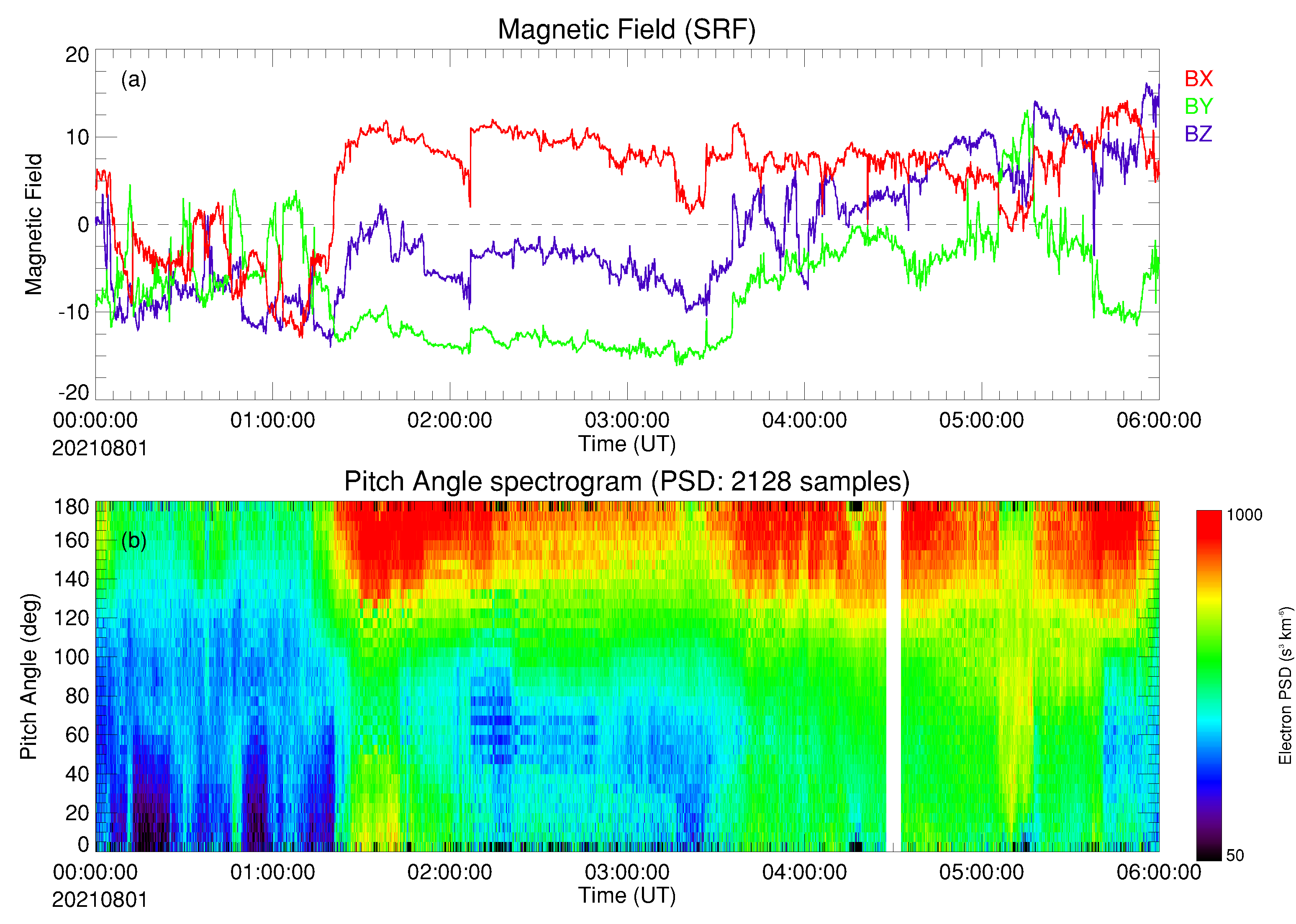
An example of the results of such a combination of the MAG and SWA-EAS data is shown in Figure 1. This figure contains 6-h of data, 0 to 6 UT, recorded on 1 August 2021. Panel (a) shows the components (red: x-component; green: y-component; blue: z-component) of the magnetic field vector in the spacecraft reference frame (SRF). From the variation of these components, it is clear that the magnetic field undergoes some significant changes of direction during the period shown. These data are used, as described above, to rebin data from the 2 EAS sensor heads, which for this period have a 10 second time cadence, into pitch angle space. Panel (b) of Figure 1 illustrates the resulting pitch-angle versus time spectrogram for the PSD of electrons in the SWA-EAS energy range above ∼70 eV.

We note in passing here a number of features that are evident in the electron pitch angle plots shown in panel (b) of Figure 1, since these are relevant to illustrate the broader study we report here. For much of the period shown, the pitch angle distribution (PAD) of the electrons is strongly enhanced in the anti-field-aligned direction (pitch angle $\alpha \sim 180{}^{\circ }$). This is consistent with a strahl beam of variable pitch angle width persisting for much of the period. This enhancement is strongest when the x-component of the field is positive in the SRF, which corresponds to the magnetic field pointing towards the Sun, and thus this enhanced beam of electrons is streaming away from the Sun. However, there are periods within the interval shown in which departures from this can be observed. These include periods of weaker fluxes at pitch angle $\alpha \sim 180{}^{\circ }$ (e.g., 0030–0050 UT) in which the field is reversed or more orthogonal to the Earth-Sun line, which may thus represent a Sunward streaming population. At other times (e.g., 0505–0520 UT) the PAD is more isotropic, with weaker variation in flux as a function of pitch angle. We note also a couple of periods in which there is a deficit in flux at pitch angle $\alpha \sim 0{}^{\circ }$ (e.g., 0010–0030 UT) compared to those seen in more perpendicular pitch angle directions (i.e., $\alpha \sim 90{}^{\circ }$).

We wish to be able to classify the various types of PAD seen for example in Figure 1 for a large volume of such data. We thus deploy a relatively simple fitting routine to each sample of the EAS data in pitch angle space as a means to quantify its major characteristics. The model PAD to which we fit each data sample is a combination of a constant background level, $P_B$, a gaussian of height $P_0$ and full-width-half- maximum $W_0$ centred on $0{}^{\circ }$ pitch angle, and a second gaussian of height $P_{180}$ and full-width-half- maximum $W_{180}$ centred on $180{}^{\circ }$ pitch angle:

$$f_{model}\left(\alpha \right)=P_B+P_{0}exp\left[\frac{-{\alpha }^2}{1.45W_0^2}\right]+P_{180}exp\left[\frac{-{\left(\alpha -{180}^{\circ }\right)}^2}{1.45W_{180}^2}\right],$$

(1)

Note that the values of $P_0$ and $P_{180}$ are allowed to take both positive and negative values, such that the fitting routine may capture both field-/anti-field-aligned enhancements, and any deficits, against a background level. To perform the fitting, we use the MPFITFUN routine in the IDL software package, which performs a Levenberg–Marquardt least-squares fit to our defined model function. We define the predominant errors as those due to Poisson counting statistics of the underlying electron counts recorded by the sensors, and propagate through the processing pipeline as the square-root of the PSD. The routine returns a residue based on the square root of the sum of the squares of the differences between each data point and the model fit. We use this to assess a quality-of-fit score based on the ratio of the net residue to the area under the PAD curve of each sample. In this work, we judge a fit to be an adequate representation of the data where this quality of fit ratio is 10% or less.

We categorise our data by calculating the difference between the average PSD for pitch angles <45${}^{\circ }$ and >135${}^{\circ }$ and the average PSD between 65${}^{\circ }$ and 115${}^{\circ }$ and comparing to that of the average near-perpendicular flux. We thus define factors $\beta$ for each field aligned direction as:

$${\beta }_{para}=\frac{\widehat{f}(0^{\circ }:{45}^{\circ })-\widehat{f}({65}^{\circ }:{115}^{\circ })}{\widehat{f}({65}^{\circ }:{115}^{\circ })},$$

(2)

$${\beta }_{antipara}=\frac{\widehat{f}({135}^{\circ }:{180}^{\circ })-\widehat{f}({65}^{\circ }:{115}^{\circ })}{\widehat{f}({65}^{\circ }:{115}^{\circ })},$$

(3)

If one or other or both of these factors is >2, then we classify the overall distribution to be one which exhibits a meaningful strahl component. Similarly, if one or other or both of these factors is <−0.5, then we class the overall distribution to have a meaningful deficit. In this way, we define the presence of a strahl beam as a field-aligned PSD exceeding the perpendicular PSD by a factor of 2 or more, and the presence of a deficit when a field-aligned PSD is less than 50% of the perpendicular PSD.

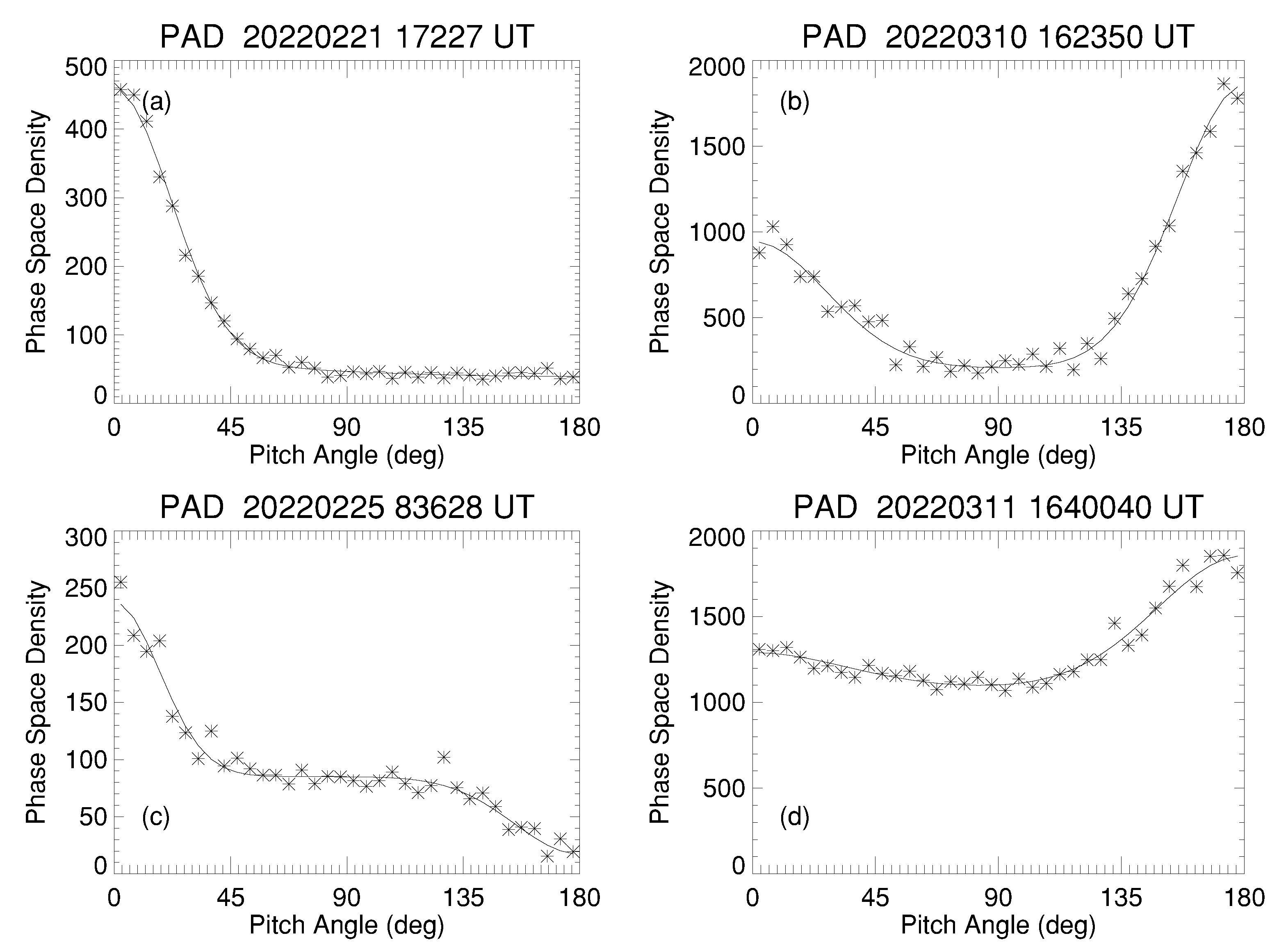
Some representative results from application of the fitting routine are shown in Figure 2. In panel (a), top left, we show a sample of data from 19 March 2022, presented as average PSD against pitch angle. The sampled data points are represented by the asterisks while the model resulting from application of our fitting scheme are shown as the solid trace. In this case, the PSD of electrons moving along the field, at 0${}^{\circ }$ pitch angle, exceeds that of the near-perpendicular fluxes by more than a factor of 2, while the PSD of the anti-parallel electrons does not. We thus classify this as an example of a uni-directional field-aligned strahl beam. Conversely, the example in panel (b), top right, shows a case from a sample recorded on 10 March 2022, in which both the field and anti-field aligned PSDs exceed the perpendicular PSD by more than a factor of 2. This is thus an example of bi-directional strahl beams. Panel (c), bottom left, shows a field-aligned beam, similar to panel (a), but in the anti-field-aligned direction there is a clear reduction in the PSD compared to that in the perpendicular direction. We thus class this as an example of a deficit in the electron population at these energies. Finally, for completeness, we show an example in which neither field-aligned direction exceeds the perpendicular flux by more than a factor of 2, so we classify this example as quasi-isotropic under our working definitions. (Similarly samples with small relative deficits which do not drop below 50% of the perpendicular flux would also be classed as quasi-isotropic—not shown here).

In this section, we have described a processing algorithm to generate a 2D pitch angle distribution from the SWA-EAS normal mode 3D data, by reference to the magnetic field direction, and defined a classification scheme by which to assess the nature of the electron population. We apply this scheme to a relatively large volume of data and describe the results of this exercise in the next section.

3. Results

We have a total of 311,696 data samples for which both EAS and MAG data are available between 1st January 2022 and 12th March 2022. We have processed these data samples along the lines described in Section 2, and present the statistics of the results in

Table 1. Occurrence statistics for strahl beams and deficits in >70 eV solar wind electron populations.

Item	Number	(%)	+ve ${\mathit{B}}_{\mathit{R}}$	(%)	−ve ${\mathit{B}}_{\mathit{R}}$	(%)
Total Measurements	311,696	(138.3%)	171,756	(55.1%)1	139,940	(44.9%) 1
Good Fits	225,302	(100%)	112,313	(49.9%)	112,989	(51.1%)
Quasi-isotropic	65,471	(29.1%)	25,815	(11.5%)	39,656	(17.6%)
Strahl, 0${}^{\circ }$ PA	83,650	(37.1%)	73,107	(32.4%)	10,543	(4.7%)
Strahl, 180${}^{\circ }$ PA	69,008	(30.6%)	9829	(4.4%)	59,179	(26.3%)
Strahl, 0${}^{\circ }$ & 180${}^{\circ }$ PA	6131	(2.7%)	2420	(1.1%)	3711	(1.6%)
Deficit, 0${}^{\circ }$ PA	9440	(4.2%)	3303	(1.5%)	6137	(2.7%)
Deficit, 180${}^{\circ }$ PA	9406	(4.2%)	6393	(2.8%)	3013	(1.3%)
Deficit, 0${}^{\circ }$ & 180${}^{\circ }$ PA	86	(0.04%)	67	(0.03%)	19	(0.01%)

¹ Of total measurements.

.

3.1. Overall Statistics for the Samples

Using the metric that the ratio of the residue for our fitting routine to the area under the fitted sample curve should be <10% for a good fit to be returned, we identify 225,302 samples, or ∼72%, of the total available samples, which are well-fitted by our simple model. The breakdown of the classifications of these fitted samples is shown in columns 1 and 2 of Table 1, with the percentages that each category represents within the well-fitted population given in column 3. From this we see that the distributions are classified as quasi-isotropic in a little under one third (29.1%) of the well-fit cases, while a similar number of strahl beams are identified in one direction or the other with respect to the field (representing 37.1% and 30.6% of the well-fit cases for the 0${}^{\circ }$ and 180${}^{\circ }$ pitch angle beams, respectively). Note that only a small number of cases, 6131 or ∼$2.7\%$ of the well-fit cases, are classed as a strahl beam both parallel and anti-parallel to the field in the same sample.

The last 3 rows of Table 1 also show the results for the characterisation of field-aligned deficits in the >70 eV electron population. These occur in a much smaller fraction of the overall well-fit dataset, with <20,000 samples (8.4%) evenly split between 0${}^{\circ }$ and 180${}^{\circ }$ pitch angle cases (both at 4.2% to 1 decimal place accuracy). An almost negligible number of fits (86, 0.04%) return a deficit in both field aligned directions.

3.2. Relation to Magnetic Field Direction

The direction of the strahl beams and other features with respect to the magnetic field vector should be put into context by considering how the field, and thus the beam, is directed with respect to the Sun. We make a relatively simple assessment of the heliospheric direction of beams by reference to the sign of the $B_R$ component of the magnetic field, in the RTN frame, at the time of each sample, and further divide the classifications accordingly. The results of this are shown in columns 4–7 of Table 1, with columns 4 and 5 showing the numbers for each class occurring during positive IMF $B_R$ and columns 6 and 7 showing those occurring during negative IMF $B_R$. We note that although there is a small difference in the total number of measurements available for the 2 IMF directions, the samples that return good fits under our definition split almost exactly in half (49.9% and 51.1% of the well-fit cases for positive and negative IMF $B_R$, respectively).

The quasi-isotropic class of samples shows a small tendency towards preferential occurrence for negative IMF $B_R$. However, as expected, the major differences occur in the strahl samples. The 0${}^{\circ }$ pitch angle beams occur with strong bias towards positive IMF $B_R$ (totalling 32.4% of the well-fit cases) compared to negative $B_R$ cases (only 4.7% of the well-fit cases). Conversely, the 180${}^{\circ }$ pitch angle beams show strong bias towards negative IMF $B_R$ (totalling 26.3% of the well-fit cases) compared to positive $B_R$ cases (only 4.4% of the well-fit cases). Given that 0${}^{\circ }$ pitch angle beams in positive $B_R$ fields and 180${}^{\circ }$ pitch angle beams in negative $B_R$ fields both travel with an outward component to their motion, we find in combination that a total of 73,107 + 59,179 samples (equivalent to 58.7% of the well fit cases) show an outward propagating strahl beam, while only 10,543 + 9829 samples (9.1% of the well fit cases) show an inward propagating, or reverse strahl beam. The bi-direction strahl class again is almost equally split between the 2 IMF cases (at 1.1% and 1.6% of the well-fit cases for positive and negative IMF $B_R$, respectively).

A similar form of disparity is also seen in the deficit class. Here samples with deficits at 0${}^{\circ }$ pitch angle in negative $B_R$ fields or deficits at 180${}^{\circ }$ pitch angle in positive $B_R$ fields occur in the sunward moving parts of the population. These occur in a total of 6137 + 6393 (equivalent to 5.5% of the well fit cases). Conversely the opposite pairs, representing a deficit in the outward moving electron population, occur in a only about half that total number of samples, 3303 + 3013 (equivalent to 2.8% of the well fit cases). Bidirectional deficits occur in too small a number for their split by IMF direction (found here in a ratio of 3.5:1) to be significant.

In the following subsections we focus on the properties of the outward moving strahl beams and the inward directed deficits in the PAD, and consider how these features vary with magnetic field strength, solar wind speed and radial distance from the Sun.

3.3. Occurrence and Pitch Angle Width as a Function Magnetic Field Strength

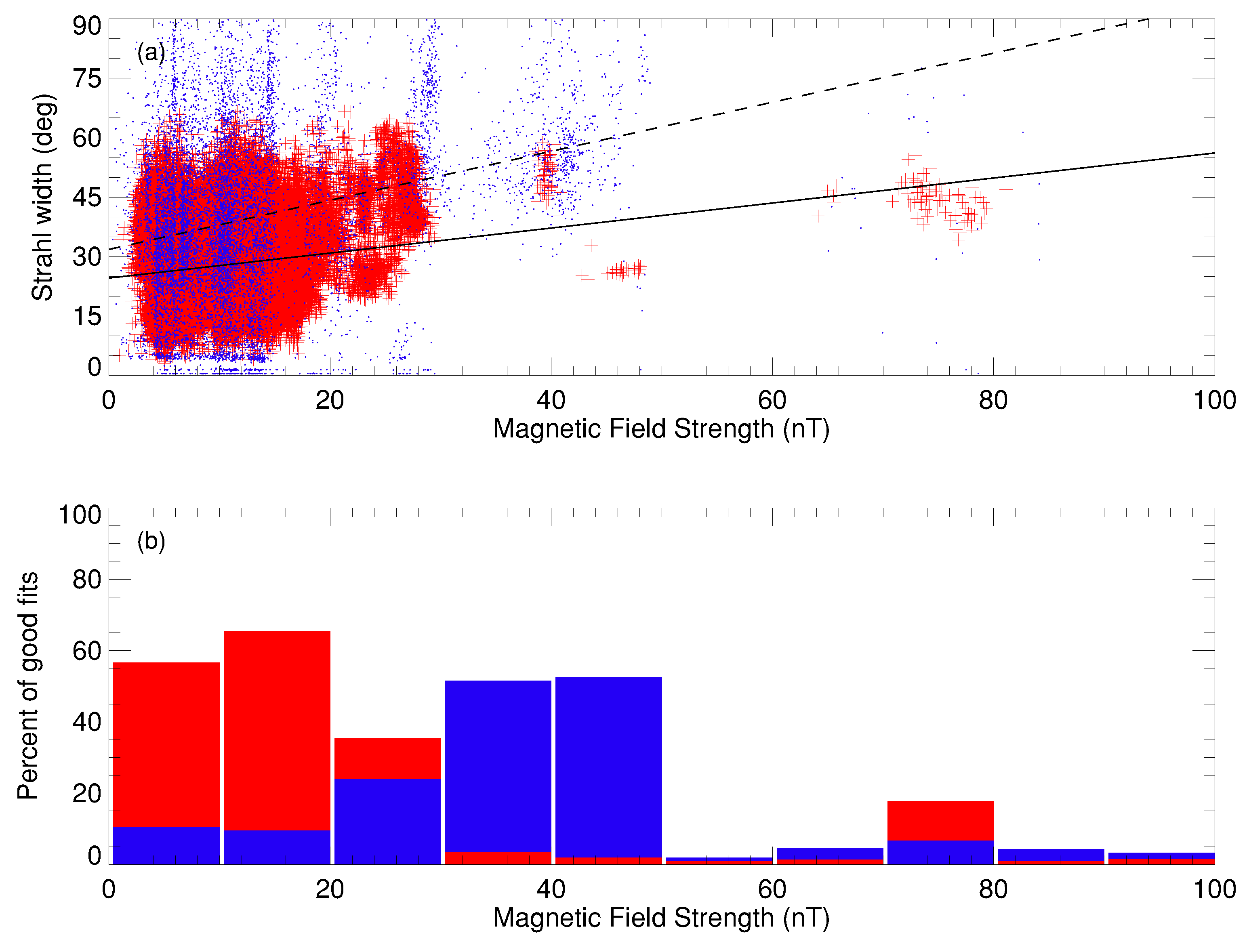
Figure 3 shows a breakdown of the occurrence of the 132,286 samples (equivalent to 58.7% of the well fit cases) which our algorithm classes as demonstrating an outward propagating field-aligned strahl beam, and the 12,688 (equivalent to 5.5% of the well fit cases) which are classed as showing a deficit in the part of the electron population in this energy range which is heading back towards the Sun, both as a function of the concurrently observed magnetic field strength. In the latter case the numbers of fits is relatively small, such that further breakdown starts to threaten the statistical significance of the results for this population. It is thus likely that a study which includes more Solar Orbiter perihelion passes will be necessary to fully confirm the related results presented here.

Panel (b) of Figure 3 shows the proportion of samples occurring as a function of magnetic field strength, in 10-nT-wide bins, as a percentage of the total number of good fits which can be associated with that bin. We represent the percentage of outward strahl beams as a red histogram and the percentage of deficits as the blue histogram. Note that the latter data has been multiplied by a factor of 2 in order to aid visualisation.

There is some suggestion that the occurrence rate of the outward strahl beam (red histogram) may fall off as the magnetic field strength increases. However, their are relatively few samples returned for field strengths >30 nT with the exception of a cluster around 70–80 nT. The distribution of the samples is more clearly seen in panel (a) of the figure, in which the red symbols plot the fitted pitch angle width of the strahl beam during each sample against the field strength for that sample. At lower field strengths, the returned PA widths of the strahl are broadly spread between ∼$5^{\circ }$ and ∼${60}^{\circ }$, although this spread narrows at higher field strengths. We determine a linear best fit straight line to this population, shown as the black solid line, which suggests that the width the beam, $W_{strahl}=24.6+0.32\left|B\right|$, or that the average strahl beam width increases with field strength at a rate of 0.32${}^{\circ }$ nT${}^{-1}$.

Similarly, the blue histogram in panel (b) of Figure 3 suggests that the deficits in PSD occur more frequently for lower field strengths, although again the statistical significance is likely to be weak. The blue points in panel (a) plot the width of the feature in each sample and show that this tends to be broader in pitch angle than the opposing strahl beam. A best fit straight line, represented by the black dashed line, $W_{deficit}=31.8+0.62\left|B\right|$, suggests the pitch angle width of the feature also increases with increasing field strength at a rate of 0.62${}^{\circ }$ nT${}^{-1}$.

3.4. Occurrence and Pitch Angle Width as a Function of Solar Wind Velocity

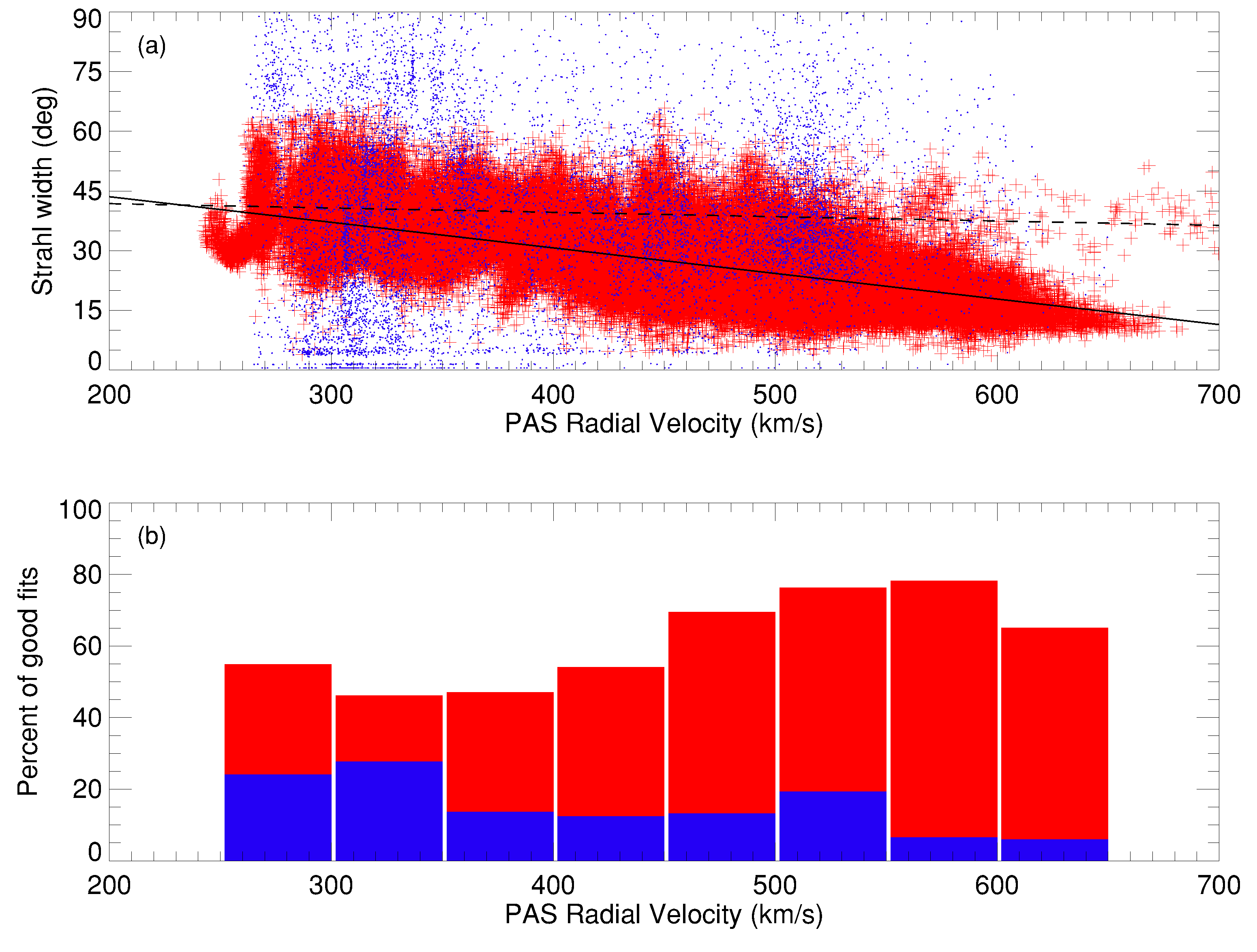
Figure 4 shows a breakdown of the occurrence of the outward propagating field-aligned strahl beam samples, and samples classed as deficits in the sunward moving part of the electron population, both now as a function of the concurrently observed solar wind speed. The latter data is extracted from the level 2 moments calculated from the ground-calibrated SWA-PAS observations, which are freely available from the SOAR. The format of the figure is otherwise the same as in Figure 3, except that the heights of the blue bars in the histogram are increased by a factor of 3 to aid clarity.

Panel (b) of Figure 4 shows the proportion of samples occurring as a function of concurrent solar wind speed, in 50 km s${}^{-1}$ wide bins, again as a percentage of the total number of good fits which can be associated with that bin. We again represent the percentage of outward strahl beams as a red histogram and the percentage of deficits as the blue histogram and again note that the latter data has been multiplied by a factor of 3 for visualisation purposes.

We note that there appears to be a steady increase in the occurrence rate of the anti-sunward strahl beam (red histogram) with solar wind velocity, rising from ∼$50\%$ under our classification at low <350 km s${}^{-1}$) flow speeds to nearer 80% at higher (>550 km s${}^{-1}$) speeds. (We note that there is some uncertainty on the SWA-PAS measurements for low flow speeds, but do not believe this has a significant impact on these binned results.) Conversely there is some suggestion from the blue histogram in panel (b) of Figure 4 that the occurrence rate of the deficit may be higher for the slower flow speeds.

Panel (a) of Figure 4 again plots the fitted pitch angle width of the individual samples, this time as a function of concurrent solar wind speed. Again, the red symbols plot the fitted pitch angle width of the anti-sunward strahl beam of each sample against flow speed, while the blue symbols plot the fitted pitch angle width of the sunward deficits. The strahl widths cover a broad range of pitch angle, up to ∼${60}^{\circ }$, but appear to show a narrowing with increasing solar wind speed. This is confirmed by the linear best fit, shown as the solid black line, which suggests that the average width the beam, $W_{strahl}=56.4-0.064\left|V_{SW}\right|$, or that the average strahl beam width decreases with flow speed at a rate of 6.4${}^{\circ }$ per 100 km s${}^{-1}$.

As previously seen, the spread of pitch angle widths for the deficit samples is broader than for the strahl, but in this case there does not seem to be a strong trend in the average width with solar wind velocity. The linear best fit to these data, shown as the dashed black line, shows that the average width of the deficit, $W_{deficit}=44.0-0.01\left|V_{SW}\right|$, so that the average width decreases with increasing flow speed at a rate of only 1${}^{\circ }$ per 100 km s${}^{-1}$.

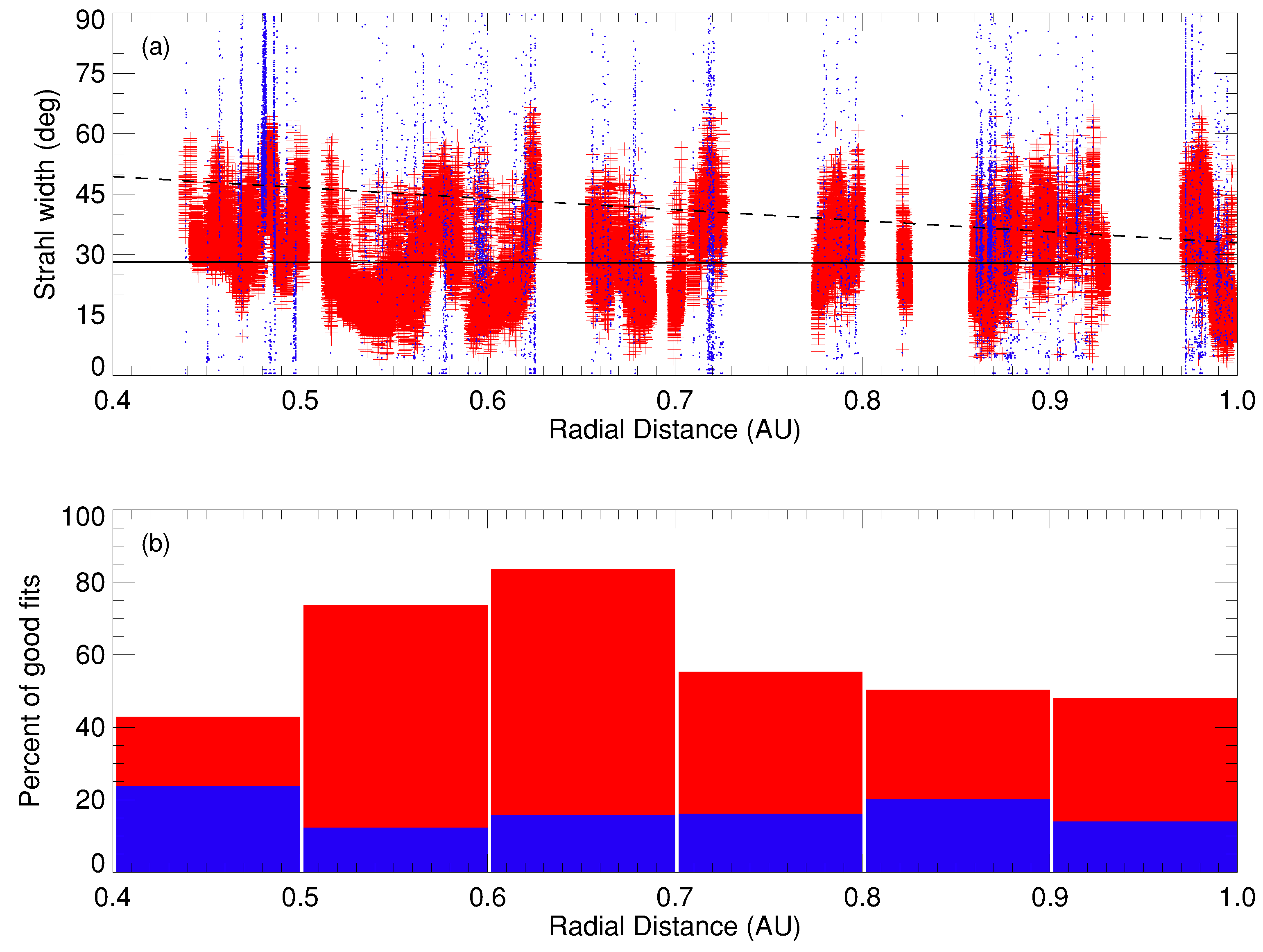
3.5. Occurrence and Pitch Angle Width as a Function of Heliocentric Distance

Finally, we consider the breakdown of the occurrence of the outward propagating field-aligned strahl beam samples, and samples classed as deficits in the sunward moving part of the electron population, as functions of the radial distance at which each sample was taken. This analysis is presented in Figure 5, which is in the same general format used in Figure 4.

The histograms in panel (b) of Figure 5 show that both the anti-sunward strahl (red bars) and sunward deficits (blue bars) occur at significant rates across the full distance range covered by Solar Orbiter during this period in which it moved inbound towards its first close perihelion. (Recall however that the level for the deficit have been increased by a factor of 3 to aid visibility). There are very high occurrence rates for the strahl between 0.5 and 0.7 AU, although care needs to be taken with interpretation as for a single inbound pass the horizontal axis is also a proxy for time. It is thus possible that some temporal change in the solar wind, not tested here, causes this peak.

The histogram for the deficit suggests that this occurs rather uniformly with distance, although we can see from panel (a) that these data occur in relatively narrow radial distance bunches, which again suggests a strong temporal variation in their occurrence. We also see in this panel that each bunch shows a relatively broad variation in fitted pitch angle width for the deficits, although the linear best fit shows a shallow decline in average deficit pitch angle width with radial distance, R, $W_{deficit}=$ 56.4 − 23.5R, or a reduction at a rate of ∼2.4${}^{\circ }$ per 0.1 AU.

The gaps in the anti-sunward strahl data points (red) are indicative of the temporal availability of the datasets underpinning this analysis. SWA-EAS data is regularly unavailable for several hours at a time due to turn-offs of the sensor to protect it against spacecraft thruster firings. In addition, some daily MAG data files are not available at the time of writing due to the need for enhanced calibration activities to remove the spacecraft generated fields from the data. However, a linear best fit to the data that are available indicates that the average pitch angle width of the strahl remains rather steady with the best fit line (solid black line in the figure) given by $W_{strahl}=$ 28.4 − 0.7R. The average strahl width for this study therefore declines by only ∼0.5${}^{\circ }$ per AU over the distance range covered by this study.

4. Discussion

In this paper, we have investigated some of the properties of the suprathermal electron population ($E\ge 70$ eV) in the solar wind inside of 1 AU. To do so we have constructed the 2D pitch angle distribution from the 3D normal mode data product returned from the SWA-EAS sensor. This is done with reference to the ground-calibrated magnetic field vector observed at the spacecraft by the MAG instrument at the time of each EAS sample. We have applied this analysis to the period of data from 1 January 2022 to 12 March 2022 as Solar Orbiter moved from near Earth space to near its first nominal mission perihelion at ∼0.3 AU.

We have used a standard fitting technique applied to a simple model of the suprathermal electron population, which considers whether, compared to an isotropic background level, there is an enhanced strahl beam at either or both of the field-/anti-field-aligned directions or alternatively whether there is a significant deficit in one or both of those directions. Following an assessment of the quality of each fit, we define these levels to be significant if the average PSD for pitch angles within a few tens of degrees of the field-/anti-field-aligned directions is a factor of 2 above (half of) the average PSD in the perpendicular directions for case of the strahl beam (deficit).

Overall we assembled a combined database with >3.1 × 10${}^5$ testable samples. Of these, around 72% returned a fit to the model that is better than the threshold we set for a sample to qualify for further analysis. Of these, around two-thirds could be classed as showing a significant uni-directional strahl beam, with a small fraction (2.7%) of these exhibiting bi-directional beams. Most of the remaining third of the samples are classed as quasi-isotropic, with only moderate variations in the PSD with pitch angle. When considered against the concurrently observed magnetic field direction, we find that most (87%) of the strahl beam cases are observed to be moving away from the Sun. This is consistent with previously reported observations (e.g., [1,3] and expectations that this population carries the majority of the heat flux away from the Sun. The remaining population (13%) are then consistent with a field aligned beam at these energies heading back towards the Sun, and may be indicative of the field configuration during ‘switchback’ events in which the IMF, and thus any associated strahl beam, is folded back on itself (e.g., [34]). Recent Parker Solar Probe [35,36] observations have shown that such structures are ubiquitous in the near-Sun (<0.3 AU) heliosphere, so the lower occurrence fraction at the Solar Orbiter distances (0.3 < R < 1.0 AU) may be representative of the survival rates of such structures as they are carried out with the solar wind. The very small fraction of events (2.7%) that show bi-directional strahl are likely to be consistent with closed magnetic loop structures, either closing on themselves as might be expected in a magnetic cloud-type structure (e.g., [37]), and/or mapping back with both feet embedded in the corona. It is also possible that some of the quasi-isotropic events occur in the magnetic cloud-type structures if the field is completely disconnected from the Sun. It may be that repeating this survey over later Solar Orbiter orbits, when the Sun is expected to be more active and producing more ejecta, will find a higher fraction of the bi-directional events.

We find that the outward directed strahl beam is observed with a higher occurrence rate during periods of faster solar wind speeds. This is also consistent with previous observations that the strahl is most readily observed during fast wind (e.g., [9]), although under our classification algorithm significant field-aligned enhancements consistent with a strahl beam are identifiable in at least 40% of cases in all speed regimes. However, we find that the strahl tends to be broader in terms of pitch angle width for slower wind speeds, so it may be that previous surveys have imposed a more limited definition of these and thus identified a smaller population at low speeds.

We find that the strahl beam is more readily identifiable for low magnetic field strengths, although this single orbit survey did not sample, or have available, many observations for field strengths above 30 nT. Again it may be that later orbits under more active solar conditions would fill in the parameter space for a similar survey. However, the data available in this survey does suggest that the average strahl pitch angle width increases with magnetic field strength, although there is a wide spread in these values. Again this is consistent with expectations that the strahl beam should narrow in pitch angle width as it moves out into lower field strength while individual electrons conserve their adiabatic invariance. However, particles with pitch angle of 30${}^{\circ }$ in a 40 nT field would focus to around 14${}^{\circ }$ when the field has dropped to 10 nT. Thus, the best fit straight line presented in Figure 3 is too shallow to be consistent with adiabatic focusing alone, and thus this represents further confirmation that scattering of the beam occurs alongside this process (e.g., [14]). Indeed this is further illustrated by the average pitch angle width trend as a function of distance, which is see in Figure 5 to be almost flat. The implication of only small changes of the nature of the strahl with distance suggests that the adiabatic focusing and scattering processes must closely counter balance each other during passage through the <1 AU heliosphere. This result is can be contrasted to previous observations (e.g., [11,12,13]) which were made at at larger radial distances than studied here. These studies indicated that the pitch angle width of the beam on average increases with radial distance, rather than remaining broadly steady. Thus, the conclusion by [14], that these observations are consistent with scattering effects dominating over adiabatic focusing, may need some modification for beams propagating between ∼0.3 and 1 AU.

As noted above, our fitting procedure is also able to identify samples in which there is a significant deficit in the field-/anti-field aligned direction when compared to the PSD at perpendicular pitch angles. There are relatively few such cases, totalling only ∼8.4% of the well-fitted samples. This may be broadly consistent with the conclusion by [27] that these structures in the distribution, while common close to the Sun, are not generally detected by PSP beyond 0.3 AU. However, we find that of order two-thirds of the fitted cases are in the sunward moving portion of the overall distribution. These cases may be remnant results of the ambipolar electric fields predicted in particular by exospheric models of solar wind acceleration (e.g., [4,21,22,23,24,25,26]). In any case, these are consistent with the structure reported by [19] and demonstrated to be consistent with the kinetic conditions required for instabilities to generate quasi-parallel whistler waves, which in turn will likely result in the filling in of the deficit itself. These factors may be the cause for the deficits here to appear in narrow clumps when plotted as a function of distance, which in this survey is closely related to time of observation. It may be that clusters of deficit holding distributions pass by the spacecraft in short bursts, having, for reasons not identified here, survived or been generated to distances well beyond the 0.3 AU reported by [27]. These clusters do not appear to have a strong occurrence association with solar wind speed or IMF field strength. Although they tend to have a broader pitch angle width than is typical of the strahl seen in this survey, their average width does slowly decrease with radial distance, which may be consistent with the deficits tending to be filled in at greater distances. Alternatively, the sunward propagation of electrons in this part of velocity space would lead to adiabatic broadening of this feature, which is consistent with the trend identified by the best fit (dashed) line in Figure 3. Again it may be that a balance of processes is needed to explain the variations of these deficits in the solar wind.

One limitation of the current study is that it is confined to data from the first inbound passage of Solar Orbiter in its nominal mission. This means that there are some gaps in parameter space and some issues with statistical significance of the data groups, particularly if further binning is required. For example, assessment of observations of bi-directional strahl (and indeed bi-directional deficits) would be interesting if more events could be identified. Fortunately, it is expected that Solar Orbiter will make 4 such transitions from 1 AU to 0.3 AU (or vice versa) per year for the next 4 to 5 years at least. Thus, it should be a useful exercise to rerun this survey in a few years time to further validate the results.

Additionally, we have focused in this paper on the energy-averaged properties of the electrons in the >70 eV range. A second development that should be undertaken as the volume of the dataset increases, such that splitting data into smaller parameter bins can be achieved without losing statistical significance, would be to examine the variation of the strahl parameters as a function of energy. Previous studies of the variation in strahl width as a function of energy have been contradictory or inconclusive (e.g., see the discussion in [13] and references therein). The balance of focusing and scattering processes may well be variable with energy depending on, for example, the instabilities involved and their resonance with electrons in a narrow energy range (see, for example, [16]). Application of the present dataset, as it develops, will allow us to take a new look at this issue with improved data products.

Finally, there are important overlaps for this dataset with the equivalent one currently being accumulated by the Parker Solar Probe mission and its SWEAP instrument [28]. The combined dataset will potentially support relevant 2 point measurements, for example during radial alignments, which will likely also improve our understanding of the evolution of the strahl electrons.

5. Summary and Conclusions

We have undertaken an assessment of the occurrence rates and characteristics of suprathermal electrons observed by SWA-EAS at energies of >70 eV during the approach of Solar Orbiter to it first close perihelion in early 2022. We find that:

• Under our classification system a significant population of anti-sunward moving strahl beams is identifiable in the tested samples;
• These beams are seen in all solar wind speed regimes, but, consistent with earlier observations, are slightly more prevalent at high speeds;
• These beams occur at all distances examined (0.4–1.0 AU), but do not show significant evolution with distance, suggesting a balance between focusing and scattering processes across the distance covered;
• Nevertheless the data suggests that the beams broaden on average with increasing magnetic field strength and narrow on average with increasing solar wind speed;
• We also identify a small population, occurring in sporadic clusters, of deficits in the sunward moving part of the electron distribution;
• These clusters occur across the distance range sampled and show some variations in average properties with radial distance, suggesting they too are influenced by competing scattering and (de-)focusing processes.

The underlying data set is expected to increase in volume over the coming years, so these results will be further tested and validated with increased statistical significance.