Single-Photon Double-Slit Interference in the 4+1 Formalism

Abstract

Unifying quantum theory with general relativity is challenging because of several problems related to time and to collapse in quantum measurements. In the double-slit experiment, the questions are how the momentum of the photon is transferred to a specific location on the screen and how the double slit recoils accordingly. This work investigates if these problems can be solved by adding a second time $\tau$, which acts as an external evolution parameter, to standard four-dimensional spacetime. Within the resulting 4+1 formalism, a model for the single-photon double-slit experiment is developed. On the one hand, each spacetime associated to a value of $\tau$ relies on classical worldlines that obey local momentum conservation. On the other hand, these worldlines are allowed to readjust as a function of $\tau$ such that the quantum phenomenon of double-slit interference can be reproduced. The model explains how determinate outcomes are produced and how momentum transfer occurs in a way that satisfies the principles of relativity and local momentum conservation. As a result, the measurement problem and the problem of time evaporate, and an explanation for our experience of the present emerges. Since the presented model succeeds in explaining a key quantum phenomenon with essentially classical worldlines, this is relevant for the field of quantum gravity.

1. Introduction

Quantum theory and general relativity are highly successful in their own domains, but when trying to merge these theories several problems arise—problems that tell us that something may be fundamentally wrong with our standard view of spacetime. One of these problems, the measurement problem, is the problem of making quantum measurements compatible with the spacetime of relativity [1,2,3]. Another problem, the problem of time, refers to a major incompatibility between the external time of quantum mechanics and the dynamic time of general relativity [4,5,6]. Additionally, it is worthwhile to mention a third issue, that our experience of the present and the flow of time may also point at a conflict with general relativity (see [7,8,9]). In the context of the single-photon double-slit experiment, the problem is with explaining how determinate outcomes are produced and how momentum is transferred in a way that is compatible with relativity and local momentum conservation. Standard quantum theory produces a probability distribution for detecting the photon somewhere on the screen. Consequently, to explain why the photon is observed at a specific location on the screen, an additional collapse mechanism is needed, which is incompatible with relativity and local momentum conservation. Additionally, other interpretations of quantum mechanics such as Bohmian mechanics [10,11] and many-worlds [12] fail to provide a satisfying solution (see [1,13,14,15]).

In this work, a theoretical framework is proposed with the aim of solving the above-mentioned problems, with a focus on the double-slit experiment. On the one hand, the presented theory stays as close as possible to the classical, single-world view of general relativity. This choice is made because general relativity accurately describes the macroscopic world and because it fits well with our perception of a single, classical world. To maximize compatibility with classical general relativity, the presented theory insists on fundamental principles such as realism and locality. It assumes that there are really existing entities in spacetime such as worldlines that interact locally and obey local momentum conservation. On the other hand, considering the above-mentioned issues with spacetime and considering that quantum mechanics rules out local realism within standard spacetime (see [16,17,18,19,20,21,22,23,24,25,26]), in this work spacetime is modified in the sense that a second type of time, denoted by $\tau$, is introduced in addition to the familiar space and time dimensions. In the resulting 4+1 (or $4D+\tau$) framework, worldlines can spatially reorient and change other properties as a function of the additional time $\tau$, in contrast to standard relativistic mechanics where worldlines consist of fixed events in four-dimensional (4D) spacetime. This dual time scheme offers much freedom to explain quantum phenomena. Together, the aim is to produce a framework that can explain observations of quantum phenomena that maximizes compatibility with the classical, single-world view of general relativity and—as a bonus—offers an explanation for our experience of the present.

The concept of a second time goes back to Broad [27] (see also [7]) and is also present (even though not mentioned explicitly) in the crystallizing block universe of Ellis and Rothman [28]. However, in this literature the past region of worldlines is assumed to be fixed while just gradually more of the worldlines comes into existence as a function of the additional time, and it is not clear how such a framework can be compatible with both quantum mechanics and general relativity. The present work aims to overcome this issue by allowing worldlines to be fully dynamic as a function of $\tau$. To some degree, there is a resemblance to Stueckelberg–Horwitz–Piron theory [29,30] (see also [31,32]) which also relies on a second time parameter (also called $\tau$). There also exist traditional retrocausal (or “future-input-dependent”) quantum models (see [33,34,35,36]), but in general, it is not well established how traditional retrocausality fits within the causal structure of standard spacetime [37]. This problem is avoided here by implementing phenomena that may appear retrocausal from the perspective of a standard observer in a fundamentally causal way as a function of the additional time $\tau$.

Within the 4+1 framework, a model is developed for the single-photon double-slit experiment, which is known to demonstrate essential quantum behavior [38]. Standard quantum mechanical or quantum field theoretical treatments of the double-slit experiment (see [39,40]) typically only produce the familiar probability distribution on a screen without explaining how determinate outcomes are obtained or how the transfer of photon momentum from source to detector and the recoil of the double slit can be made compatible with relativity and local momentum conservation. The presented model offers an explanation for these matters with an ontology of worldlines that are dynamic as a function of $\tau$. In essence, each photon is represented by worldlines that spatially readjust as a function of $\tau$ to produce a spatial density that matches the desired quantum probability distribution. One randomly selected worldline determines the outcome of the experiment and locally transfers recoil momentum to the double slit. In this way, determinate outcomes are produced in agreement with the quantum probability distribution, explaining wave–particle duality. Furthermore, momentum transfer between the photon and the double slit occurs such that at each value of $\tau$ before and after measurement all worldlines obey local momentum conservation. Therefore, a classical but $\tau$-dependent energy-stress tensor is obtained that is compatible with classical relativistic mechanics, explaining the quantum-to-classical transition. It is shown that in this framework the problems of measurement and time evaporate and that an explanation can be given for our experience of the present and the flow of time. Additionally, it is discussed that the addition of a second time parameter may offer an interesting path towards a unified theory of quantum gravity.

2. Theoretical Framework

2.1. A Modified Spacetime

In this work, 4D spacetime is supplemented with a second form of time represented by the scalar $\tau$. For each value of $\tau$, there is an associated four-dimensional spacetime $M\left(\tau \right)$ with metric $g\left(\tau \right)$. Mathematically, this results in a $M_5=M\times \mathrm{I}\mathrm{R}$ structure that can be described as an ordered, continuous set of Lorentzian manifolds $\{M\left({\tau }_1\right),M\left({\tau }_2\right),\dots \}$ with corresponding metrics $\{g\left({\tau }_1\right),g\left({\tau }_2\right),\dots \}$, labeled with values of the scalar $\tau \in \mathrm{I}\mathrm{R}$. The interpretation is that standard 4D spacetime M is combined with a scalar evolution parameter $\tau$ to obtain a $\tau$-dependent 4D block universe $M\left(\tau \right)$. Such four-dimensional spacetime with the external evolution parameter $\tau$ results in a ($4D+\tau$)-structure, or 4+1 for short. Each 4D spacetime $\left(M\right(\tau ),g(\tau \left)\right)$ satisfies the Einstein field equations and momentum conservation. To avoid confusion using terminology normally associated with time t, the prefix “$\tau$-” is used to explicitly specify when dynamics as a function of $\tau$ are considered. Notice that the 4+1 framework is not the same as a five-dimensional spacetime, in which there would be extra space or time coordinates. The problem of time mentioned in the introduction originates precisely from the fact that time in general relativity is reduced to merely a coordinate such that spacetime becomes a static four-dimensional structure. In the 4+1 formalism, $\tau$ re-introduces the analog of an external, absolute time as encountered in classical and quantum mechanics into standard four-dimensional spacetime.

Physically existing entities are characterized by events of the form $x^{\mu }\left(\tau \right)$, where the coordinates $x^{\mu }$ for $\mu =0,1,2,3$ correspond respectively to $x,y,z,t$. It is therefore assumed that the same physical entities exist in different 4D spacetimes associated with the evolution parameter $\tau$. If the coordinate systems of all spacetimes are chosen wisely, namely such that the coordinates of the elements of reality also vary continuously as a function of $\tau$, then the path of an element of reality as a function of $\tau$ can be described by a function $f:\tau \to {\mathrm{I}\mathrm{R}}^{3,1}$ that maps values of $\tau$ onto four-dimensional coordinates with signature $(3,1)$.

Furthermore, worldlines in 4D spacetime that are dynamic as a function of $\tau$ are considered. If individual physical entities constituting a worldline are described as $\tau$-dynamic events $x^{\mu }\left(\tau \right)$, then the general form of a $\tau$-dynamic worldline is $x^{\mu }(\lambda ,\tau )$. This means that at each value of $\tau$ (which specifies the evolution) there is a spacetime $M\left(\tau \right)$ in which the worldline is characterized by a set of events of the form $x^{\mu }\left(\lambda \right)$ with affine parameter $\lambda$ pointing at these different events as usual in relativistic mechanics. Notice that, in contrast, a standard worldline in ordinary spacetime is simply characterized by events $x^{\mu }\left(\lambda \right)$ with affine parameter $\lambda$ pointing at individual events. Hence, starting from such a standard worldline $x^{\mu }\left(\lambda \right)$, it makes sense to add the evolution parameter $\tau$ to make each event $\tau$-dynamic, and as a result also the whole worldline. There are certain restrictions in the freedom of $\tau$-dynamic worldlines. One restriction for worldlines carrying energy and momentum comes from the Einstein equations, which impose that there is conservation of energy and momentum in each spacetime $\left(M\right(\tau ),g(\tau \left)\right)$. Physical interactions governed by matter equations can further limit the freedom of worldlines.

Additionally, a physically preferred hypersurface $\Sigma \left(\tau \right)$ is introduced that shifts the time dimension in the positive direction as $\tau$ increases. This hypersurface forms the boundary between a past region of spacetime containing $\tau$-dynamic worldlines and a future spacetime region in which worldlines are not yet formed—even though building blocks of these worldlines may already be present there. 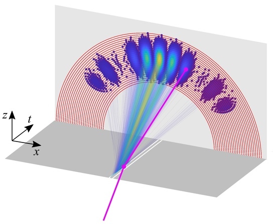Hence, it is implied that $\Sigma \left(\tau \right)$ itself is associated with the present. A schematic illustration of this concept is shown in Figure 1a. Here, each spacetime $\left(M\right(\tau ),g(\tau \left)\right)$ is split up into two regions separated by a spatial hypersurface $\Sigma \left(\tau \right)$. At each value of $\tau$ the corresponding hypersurface $\Sigma \left(\tau \right)$ is designed such that it contains the endpoints of all involved particle worldlines (dots in Figure 1a). As the value of the evolution parameter $\tau$ increases, the worldlines grow in a synchronized way while the hypersurface $\Sigma \left(\tau \right)$ advances in the positive direction of the time dimension. It is assumed that far in the past region worldlines are largely constrained by interactions, producing what one could call a crystallized region (yellow region). However, close to the hypersurface $\Sigma \left(\tau \right)$ (blue region), the growing ends of the worldlines still have freedom to reorient in four-dimensional spacetime as a function of $\tau$, as long as overall energy and momentum conservation is satisfied in each spacetime and the matter equations allow it. This freedom will turn out to be crucial for explaining quantum phenomena. In the region to the future of $\Sigma \left(\tau \right)$, worldlines are not yet formed (white region). In this region, building blocks of worldlines may be present in a still unorganized way.

If we assume that at some value $\tau$ the region sufficiently to the past of $\Sigma \left(\tau \right)$ has reached a rigid configuration (yellow region in Figure 1a), then the dependency with $\tau$ can be ignored in this region such that this region can be described as a part of a standard (not $\tau$-dependent) spacetime $(M,g)$, satisfying the Einstein field equations and the associated matter equations. When more of spacetime becomes crystallized as $\tau$ increases, this metric can be further extended up to the new hypersurface $\Sigma \left(\tau \right)$ while the previously crystallized part of the metric remains identical. In the limit of $\tau \to \infty$ the entire spacetime becomes crystallized and approximates a traditional, fixed spacetime $(M,g)$ as it appears in classical general relativity. Standard observers in the $(4D+\tau )$ framework, that in fact also consist of $\tau$-dynamic worldlines, can make observations in the form of measured events $x^{\mu }$ and can map these events out in ordinary spacetime. However, the $\tau$-dynamics of worldlines that occur before a measurement cannot be directly observed. Only the final interaction event can be inferred with standard measurement techniques. The resulting standard 4D spacetime $(M,g)$ in agreement with classical general relativity, as it appears according to a standard observer, is illustrated in Figure 1b. Therefore, by construction, the macroscopic observations agree with classical general relativity, as is desired. In fact, in the 4+1 framework all features of classical relativistic mechanics can be easily reproduced. It suffices to block $\tau$-dynamics in the past region of the hypersurface $\Sigma \left(\tau \right)$ and to allow only local interactions that conserve momentum. In this case, as $\tau$ increases and $\Sigma \left(\tau \right)$ shifts in the positive direction of the time dimension, an increasing part of a standard spacetime of general relativity is revealed.

Next, by allowing $\tau$-dynamics of worldlines, it is demonstrated that quantum phenomena can also be reproduced, more specifically double-slit interference.

2.2. The Double-Slit Experiment

Within the 4+1 framework described above, a model for the single-photon double-slit experiment is developed. For simplicity, the theory further restricts to a 4+1 structure based on flat 4D spacetime. On the small spatial scales considered in this work, $\Sigma \left(\tau \right)$ is assumed to be a flat hypersurface that picks out a preferred coordinate system. The spatial geometry consists of a photon source at position $(x_S,y_S,z_S)$ along the negative z-axis (namely $x_S=y_S=0$, $z_S<0$), a double-slit aperture in the $(x,y)$ plane and a screen or detector situated at positive z values (unspecified for the moment). Even though the double-slit experiment is spatially a 3D problem, for simplicity and without losing generality the analysis of the photon propagation behind the double slit is restricted to the $(x,z)$ plane and polarization is ignored. Only the case of a stationary double-slit experiment in the preferred frame linked to the hypersurface $\Sigma \left(\tau \right)$ is analyzed. In this preferred frame, for a general worldline $x^{\mu }(\lambda ,\tau )$ one can choose $\lambda ={\lambda }_s$ to correspond with the start event ($x_s\left(\tau \right),y_s\left(\tau \right),z_s\left(\tau \right),t_s\left(\tau \right)$) and $\lambda ={\lambda }_e$ with the end event ($x_e\left(\tau \right),y_e\left(\tau \right),z_e\left(\tau \right),t_e\left(\tau \right)$) in each spacetime associated to a value of $\tau$. Since the hypersurface $\Sigma \left(\tau \right)$ contains the end events of all worldlines, it is characterized by the time coordinate $t_e\left(\tau \right)$. As $\tau$ increases, all worldlines grow in the positive direction of the time dimension at the same rate according to $t_e\left(\tau \right)=\beta \tau$, with $\beta$ a positive scalar. The source emits a single photon characterized in the rest frame by a wavelength ${\lambda }_{photon}$ and corresponding energy $E_{photon}=hc/{\lambda }_{photon}$. Two sets of worldlines are created by the source, a “wave network” with $N_w$ worldlines and a “particle network” with $N_p$ worldlines. Worldlines from these two networks are referred to respectively as wave worldlines and particle worldlines. To model a Gaussian wave packet, the number of worldlines created as a function of time in the rest frame follows a Gaussian distribution with a central emission time of $t_S$ and a standard deviation of ${\sigma }_S$.

Below, the configuration of wave and particle worldlines is analyzed at a specific value of $\tau$. The main strategy is as follows. The value of $\tau$ specifies the time coordinate $t_e\left(\tau \right)=\beta \tau$ of the hypersurface $\Sigma \left(\tau \right)$, constraining the spatial lengths of all involved worldlines. Under this constraint, the configuration of worldlines is governed by a set of equations. This configuration can be seen as a quasi-steady-state situation under the assumption that the $\tau$ interval $\Delta \tau$ required for reaching equilibrium is much shorter than what is needed for the worldlines to grow significantly, i.e., $\Delta \tau \ll {\lambda }_{photon}/\beta c$. The description below focuses on values of $\tau$ for which most worldlines have already passed the double slit, but the theory can be applied for all values of $\tau$.

The model insists that all particle and wave worldlines are geodesic, or straight in the present case of flat spacetime, in the absence of interactions with either double slit or detector. The piecewise straight segments can be implemented by minimizing the functional $S_{geodesic}$:

$$S_{geodesic}=\int \sqrt{{\eta }_{\mu \nu }\frac{d{x}_j^{\mu }}{d\lambda }\frac{d{x}_j^{\nu }}{d\lambda }}d\lambda$$

(1)

This is the case because, for a single worldline with coordinates $x^{\mu }\left(\lambda \right)$, Equation (1) leads to the constraint $\frac{d^{2}x}{d{\lambda }^2}=\frac{d^{2}y}{d{\lambda }^2}=\frac{d^{2}z}{d{\lambda }^2}=\frac{d^{2}t}{d{\lambda }^2}=0$, which represents a straight line. Here, $\eta$ is the Minkowski metric of flat spacetime and since we are describing a photon, it is imposed that all wave and particle worldlines are piecewise null geodesics.

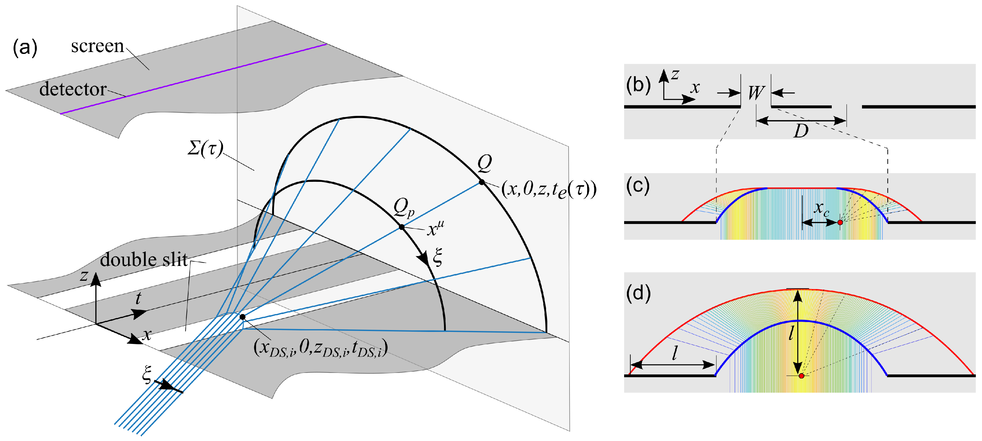
The wave network is used to produce a measure Q for the probability of finding the photon in the hypersurface $\Sigma \left(\tau \right)$ that agrees well with standard quantum theory. The approach is similar to the path integral formalism, but relies solely on null geodesic wave worldlines. Figure 2 schematically shows the geometry of a single wave worldline. Wave worldlines emanate spatially isotropically from the source in its rest frame. Considering the small dimensions of the double-slit aperture and the long distance from the source, wave worldlines are incident on the double slit in a quasi-parallel bundle along the z axis. Since the model focuses on photon propagation in the $(x,z)$ plane behind the double slit, a simple scattering model is adopted. Worldlines that pass through the double-slit openings are scattered (deflected) spatially only in the x direction while there is no deflection in the y direction. The deflection angle $\theta$ is assumed to be random with a uniform probability $\theta \in [-\pi /2,\pi /2]$ in the rest frame with respect to incidence. Based on this scattering model, the number of wave worldlines that arrive in a finite surface area $\Delta S=\Delta x\Delta y$ near the position $(x,0,z,t_e\left(\tau \right))$ in the hypersurface $\Sigma \left(\tau \right)$ (blue square in Figure 2) can be estimated as follows. From the target position $(x,0,z,t_e\left(\tau \right))$, several paths i can be traced back to the double-slit aperture and further back to the source. For path i, the deflection event at the double slit is $(x_i,0,0,t_{DS,i})$, with $x_i$ the position in the double-slit aperture and $t_{DS,i}=t_e\left(\tau \right)-\sqrt{{(x-x_i)}^2+z^2}/c$ the corresponding time coordinate. The emission event at the source is $(0,0,z_S,t_i)$, with $t_i=t_{DS,i}-\sqrt{x_i^2+z_S^2}/c$. The number of wave worldlines $N_i$ that approximately follow path i and that pass through a similar area $\Delta S$ at the position $(x_i,0,0,t_{DS,i})$ (green square in Figure 2) is:

$$N_i=N_{w,e}\left(t_i\right)\left(\frac{\Delta S}{4\pi l_{source,i}^2}\right)\left(\frac{\Delta x\cos \left(\theta \right)}{\pi l_i+\Delta x}\right)$$

(2)

Here, the first factor, $N_{w,e}\left(t_i\right)$, represents the number of wave worldlines emitted by the source at the time $t_i$ associated with path i taking into account the Gaussian wave packet produced by the source:

$$N_{w,e}\left(t_i\right)=N_w\frac{e^{-\frac{{(t_i-t_S)}^2}{2{\sigma }_S^2}}}{{\sigma }_S\sqrt{2\pi }}$$

(3)

The second factor in Equation (2) accounts for the 3D dilution before the double slit, where $l_{source,i}=\sqrt{x_i^2+z_S^2}$ is the spatial distance from the emission event at the source to the deflection point at the double slit. A good approximation is $l_{source,i}=\left|z_S\right|$. The last factor in Equation (2) accounts for the 2D dilution behind the double slit, where $l_i=\sqrt{{(x-x_i)}^2+z^2}$ is the remaining spatial distance to the event $(x,0,z,t_e\left(\tau \right))$ in the hypersurface $\Sigma \left(\tau \right)$. For large values of $l_i$, this factor reduces to $\Delta x\cos \left(\theta \right)/\pi l_i$, which represents the fraction of the angle $\Delta x\cos \left(\theta \right)/l_i$ under which worldlines are incident on the surface area $\Delta S$ at position $(x,0,z,t_e\left(\tau \right))$, to the full angle $\pi$ of all outgoing worldlines. For small values of $l_i$ at positions $(x,z)$ approaching $(x_i,0)$, this factor reduces to 1 as is desired because there is no dilution behind the double slit. Each worldline i also has a total path length $L_i=l_{source,i}+l_i$ between the source event and the end event at $\Sigma \left(\tau \right)$, with corresponding phase ${\varphi }_i$:

$${\varphi }_i=2\pi \frac{L_i}{{\lambda }_{photon}}=2\pi \frac{(l_{source,i}+l_i)}{{\lambda }_{photon}}$$

(4)

A suitable measure for probability Q at coordinates $(x,z)$ in $\Sigma \left(\tau \right)$ is defined as:

$$Q(x,z)=\sum _{p=1}^K\sum _{q=1}^K\sqrt{N_p{N}_q}\cos ({\varphi }_p-{\varphi }_q)$$

(5)

where the double summation goes over K paths from source, via positions $x_i$ (with $i=1,\dots ,K$) in the double-slit aperture separated by a distance $\Delta x$, to the position $(x,0,z,t_e\left(\tau \right))$ in $\Sigma \left(\tau \right)$. Equation (5) has similarities with the path integral formalism in that it also depends on paths through the double-slit aperture and their phases. In fact, in the far field, paraxial approximation, Equation (5) becomes identical to the following typical path integral:

$$Q_{PI}(x,z)=N{|\sum _{p=1}^K{e}^{i{\varphi }_p}|}^2$$

(6)

since in this case $N\approx \sqrt{N_p{N}_q}$ becomes a constant density of worldlines. The main reason why Equation (5) is preferred here is because it is based solely on null geodesic worldlines, it is expressed explicitly without imaginary numbers and it produces a measure for probability that scales as desired under Lorentz transformations (see [41]).

Next, the configuration of particle worldlines is determined, as illustrated in Figure 3a. Since we are interested in photon propagation in the $(x,z)$ plane, only particle worldlines in the $(x,z)$ plane (with $y=0$) are considered. The aim is to organize the particle worldlines such that their endpoints in the hypersurface $\Sigma \left(\tau \right)$ have a spatial density in the $(x,z)$ plane that is in good approximation proportional to the quantum distribution $Q(x,z)$. There are many ways in which one could arrange the particle worldlines in such a way. Here, a mechanism is chosen that not only determines the end events of the particle worldlines but the entire worldlines. Particle worldlines are chosen to emanate from the source in discrete subgroups, labeled p, which are associated to uniformly spaced emission times $t_i$ and that behave independently from each other. For each subgroup p, many particle worldlines are emitted in the same emission event $(0,0,z_S,t_i)$ at the source. Similar to the wave network with Equation (3), the number of particle worldlines emitted at time $t_i$ follows a Gaussian distribution in time centered around $t_S$ with a standard deviation of ${\sigma }_S$. The spatial density of particle worldlines ${\rho }_p\left(x^{\mu }\right)$ of one subgroup p, defined as the number of worldlines per unit distance along a curve orthogonal to the particle worldlines near the event $x^{\mu }$, is determined such that it satisfies:

$$\mathbf{n}·\mathbf{\partial }(\frac{Q_p\left(x^{\mu }\right)}{{\rho }_p\left(x^{\mu }\right)})=0$$

(7)

Here, $\mathbf{n}$ is a four-vector orthogonal to the worldlines, ∂ is the four-gradient, and $Q_p\left(x^{\mu }\right)$ takes the scalar value equal to $Q(x,0,z,t_e\left(\tau \right))$ sampled at the end event of the worldline passing through coordinates $x^{\mu }$. Along an orthogonal curve labeled by a suitable coordinate $\xi$ as shown in Figure 3a, Equation (7) simplifies to:

$$\frac{d}{d\xi }(\frac{Q_p\left(\xi \right)}{{\rho }_p\left(\xi \right)})=0$$

(8)

where $x^{\mu }$ has been replaced by the corresponding value of $\xi$ along the orthogonal curve. This demonstrates that along an orthogonal curve labeled with coordinate $\xi$ (see Figure 3a), $Q_p\left(\xi \right)/{\rho }_p\left(\xi \right)$ is constant, or in other words, ${\rho }_p\left(\xi \right)$ is proportional to $Q_p\left(\xi \right)$. As a consequence, the spatial density of particle worldlines along an orthogonal curve, and in good approximation the spatial distribution of the endpoints of the particle worldlines in $\Sigma \left(\tau \right)$, are proportional to the quantum distribution Q, as is desired. For each orthogonal curve, the value of the constant $Q_p\left(\xi \right)/{\rho }_p\left(\xi \right)$ is automatically known from the additional boundary condition that the worldlines tend to fill the entire forward hemisphere in order to minimize the local worldline density. With this boundary condition, the spatial distribution of particle worldlines along an orthogonal curve satisfying Equation (8) becomes:

$${\rho }_p\left(\xi \right)=N_{p,e}\left(t_i\right)\frac{Q_p\left(\xi \right)}{\int Q_p\left(\xi \right)d\xi }$$

(9)

Here, $N_{p,e}\left(t_i\right)$ is a similar density of worldlines emitted by the source at the corresponding time $t_i$ as in Equation (3), but for a total of $N_{p,p}$ particle worldlines that pass one of the slits. The important consequence of Equation (9) is that ${\rho }_p\left(\xi \right)/N_{p,e}\left(t_i\right)$ turns out to be a properly normalized probability distribution that is proportional to the quantum measure $Q_p\left(\xi \right)$. It also means that the parallel incoming particle worldlines are forced to spread out and to fill the entire space behind the double slit without overlapping each other, as is illustrated in Figure 3a. Since for all orthogonal curves the scalars $Q_p\left(\xi \right)$ are related to the same scalars Q at the endpoints of the associated worldlines, a similar spatial density is expected along all orthogonal curves.

Since Equation (1) insists that particle worldlines are piecewise geodesic, it is proposed that a sharp transition occurs from parallel incoming worldlines to radially outgoing worldlines at a single disclination line (see Figure 3b–d). In both regions before and after the double slit the worldlines are null geodesics and there is a single spatial deflection at the disclination line near the double slit. A suitable disclination line (independent of the y direction) that enables to connect bundles of parallel incoming and radially outgoing worldlines for the subgroup emitted at source time $t_i$ is expressed by coordinates $(x_{DS,i},z_{DS,i},t_{DS,i})$ satisfying:

$$\begin{array}{c}\hfill z_{DS,i}\left(x_{DS,i}\right)=(|x_{DS,i}\pm \frac{D}{2}|-x_c)\tan (\frac{\pi }{2}\frac{\frac{W}{2}-|x_{DS,i}\pm \frac{D}{2}|}{\frac{W}{2}-x_c})\\ \hfill t_{DS,i}\left(x\right)=t_i+\frac{|z_S|}{c}+\frac{z_{DS,i}\left(x_{DS,i}\right)}{c}\end{array}$$

(10)

as illustrated in Figure 3b–d. This disclination line is limited to $x_{DS,i}$-values that are, to the left and to the right of the center of the slits, closer than $W/2$ but further than $x_c$, where $x_c=$ max$(W/2-l\pi /2,0)$. In these (in total) four regions, worldlines spread out spatially radially from virtual centers located at $x=-D/2\pm x_c$ and $+D/2\pm x_c$ on the x axis. As a result, a typical particle worldline passing through the double-slit aperture at position $x_{DS,i}$ experiences a single interaction event $(x_{DS,i},0,z_{DS,i},t_{DS,i})$ governed by Equation (10) and ends at the hypersurface $\Sigma \left(\tau \right)$ in the event $(x,0,z,t_e\left(\tau \right))$ (see Figure 3a). For each subgroup, the spatial length of the particle worldlines between the double slit and the hypersurface $\Sigma \left(\tau \right)$ is $l=c(t_e\left(\tau \right)-t_i)-\left|z_S\right|$. 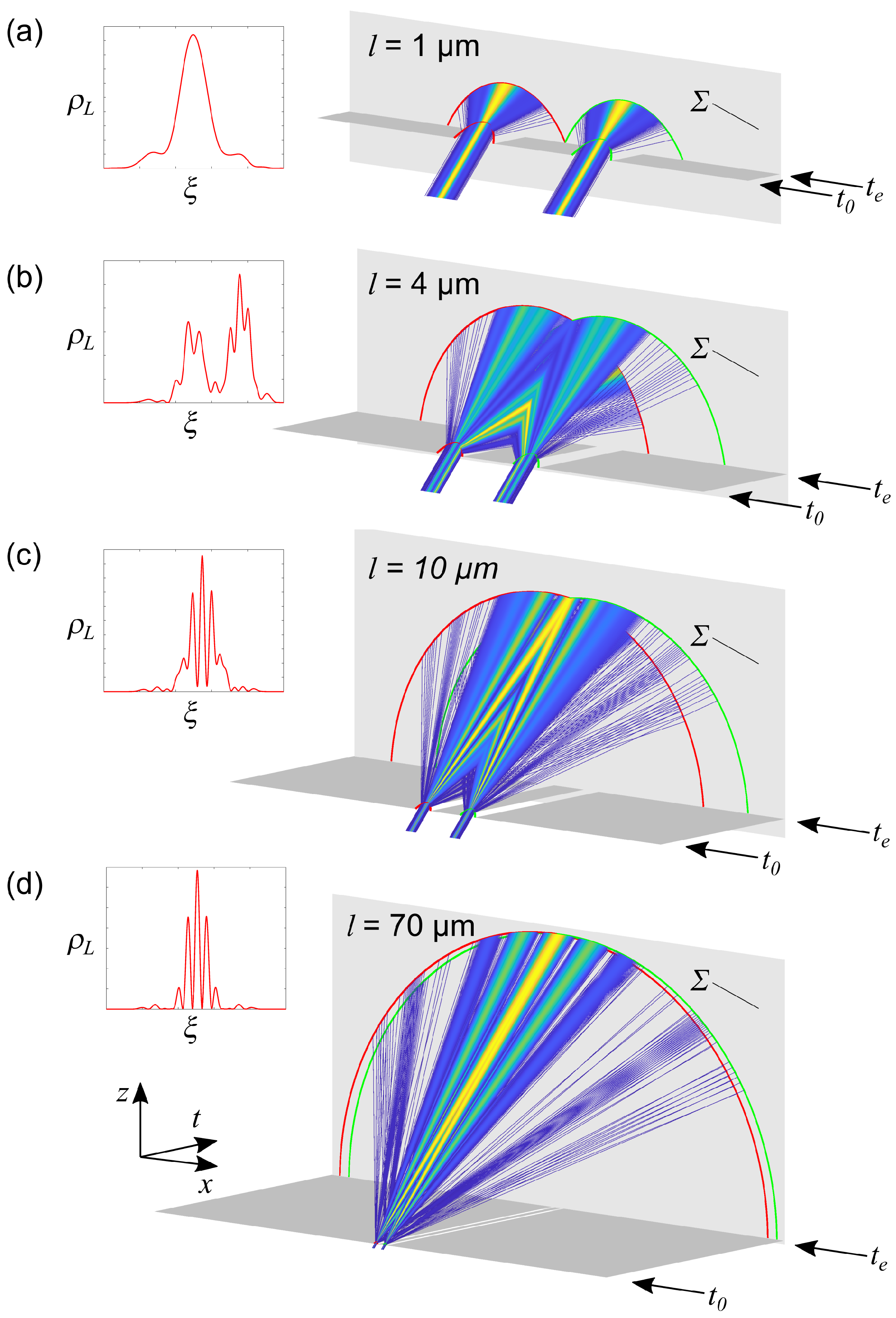If the particle worldlines have a spatial length l beyond the double slit larger than $W/\pi$, then $x_c=0$ is such that the worldlines are radiating outwards from virtual points at the center of the corresponding slit, namely at $(x,z)=(\pm D/2,0)$ (see Figure 3d). If their lengths l are shorter than $W/\pi$, then there are two regions at the left and right side of each slit (see Figure 3c). In these regions, the worldlines have a spatial angle in the $(x,z)$ plane with respect to the z axis that changes smoothly from 0 to $\pm \pi /2$, with the ± sign corresponding to the right or left side of each slit. In all cases, the shape of the disclination line ensures that the different regions before and after the double slit can be connected through piecewise straight paths. It also means that the x position of an incoming path is automatically linked to the spatial angle of the corresponding outgoing path.

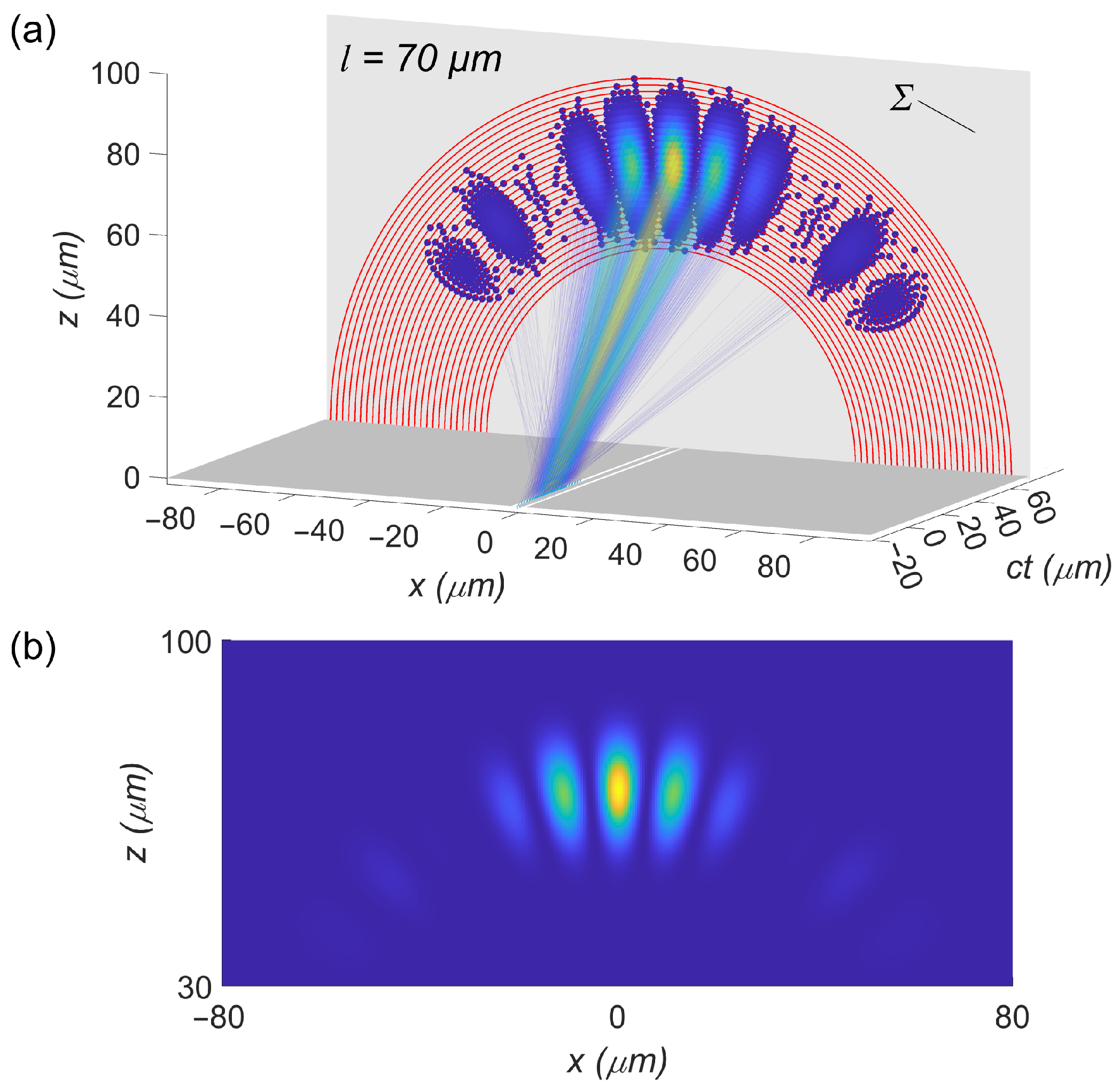
Now, it is verified to which extent the chosen disclination line in Equation (10) is compatible with Equations (1) and (7) (or Equation (9)). In the far field, which occurs for large values of l and sufficiently far from the interaction region with the double slit, each subgroup of particle worldlines passing one of the slits falls in good approximation on a single light cone. In this case, in the rest frame, all orthogonal curves are semicircles with spatial radii $R\left(t\right)=c(t-t_{start})$ increasing as a function of the time coordinate t with respect to the time $t_{start}$ corresponding to the tip of the light cone. Therefore, for all orthogonal curves a similar spatial distribution of worldlines is obtained with Equation (7) (or Equation (9)), except that it is spatially stretched and normalized differently since the spatial length of each orthogonal curve $\pi R\left(t\right)=\pi c(t-t_{start})$ increases proportionally with time t. As a result, the organization of particle worldlines is indeed compatible with straight worldlines, as is preferred from Equation (1). In the near field and close to the double slit, particle worldlines of one subgroup do not exactly follow a single light cone because of the chosen shape of the disclination line. Equation (7) then actually prefers a slight deviation from straight worldlines in the region close to the double slit, such that in a more detailed analysis of this region, more than one disclination line is needed. However, if the geodesic contribution from Equation 1 is dominant in this region, the worldlines may still prefer to be straight up to the disclination line of Equation (10). For simplicity, the latter will be assumed.

Under the above assumptions, a consistent model for particle worldlines is obtained. The regions of parallel incoming and radially outgoing worldlines consist of straight worldlines as desired by Equation (1) and are connected at a single disclination line (Equation (10)). Within each region, the spatial distribution is governed by Equation (7) (and Equation (9)). Since the spatial density distribution of particle worldlines along different orthogonal curves is essentially the same (apart for the radial expansion after the double slit) it suffices to calculate this distribution once for a single slit and for an orthogonal curve with coordinate $\xi$ chosen sufficiently far from the disclination line. A convenient choice is to select an orthogonal curve in the region of the parallel incoming worldlines for one slit. Then, based on the resulting distribution ${\rho }_L\left(\xi \right)$ (for the left slit), the full geometry of the particle worldlines can immediately be calculated using the shape of the disclination line and the basic geometry shown in Figure 3.

3. Results

3.1. Simulation of the Double-Slit Experiment

Based on the 4+1 model of the double-slit experiment developed above, simulations are carried out of the configuration of particle worldlines at different values of the evolution parameter $\tau$. Parameters of the double slit and photon are $W=1$ μm, $D=3$ μm, ${\lambda }_{photon}=500$ nm, $z_S=-1$ m, and ${\sigma }_S=50$ fs. Figure 4a shows a simulation result for the complete wave packet at one specific value of $\tau$ for which the center of the wave packet passes a distance $l=70$ μm beyond the double slit. Simulations are carried out as follows. First, the chosen value of $\tau$ determines the time coordinate $t_e\left(\tau \right)=\beta \tau$ of the hypersurface $\Sigma \left(\tau \right)$. However, rather than specifying $\tau$ and $\beta$, for simplicity the time coordinate $t_e$ itself is chosen directly. Knowing the central emission time $t_S$ of the photon wave packet and the corresponding time of arrival at the double slit $t_0=t_S+\left|z_S\right|/c$, the distance $l=c(t_e\left(\tau \right)-t_0)$ traveled by the center of the wave packet beyond the double slit can be calculated. This distance l is used to indicate the evolution of the photon as a function of $\tau$ (for example $l=70$ μm in Figure 4a). Next, the configuration of particle worldlines is determined for the 27 subgroups with emission times $t_i$ in the interval $[-3.5{\sigma }_S,+3.5{\sigma }_S]$ around the central emission time $t_S$. Outside this interval, the number of emitted worldlines becomes negligible. The red half-circles in Figure 4a indicate these discrete subgroups of particle worldlines that lie in good approximation on single light cones. Only particle worldlines passing the left slit are considered further because the result for the other slit is analogous. For each subgroup, the emission time $t_i$ determines the number of particle worldlines according to a Gaussian distribution around the central emission time $t_S$ and with standard deviation ${\sigma }_S$. In the center of the wave packet this amounts to about 1600 worldlines per slit, while the overall number for the complete wave packet is 15,000 per slit (only a fraction of the worldlines is plotted for clarity). For each subgroup, an orthogonal curve with coordinate $\xi$ is chosen in the region of the incoming particle worldlines that pass through the left slit, as illustrated (for the right slit) in Figure 3a. Since the particle worldlines in this region are parallel to the z direction, this orthogonal curve is a straight line in the x direction. Therefore, the $\xi$ coordinate is identical to the x coordinate, with values between $-D/2-W/2$ and $-D/2+W/2$ for the left slit. For the calculation of the spatial density ${\rho }_L\left(\xi \right)$, a set of incoming worldlines uniformly spaced in the x direction is first considered. Based on the known disclination line (Equation (10)), for each incoming worldline at coordinate $\xi$, there is a known outgoing worldline. At the endpoint of each worldline in the hypersurface $\Sigma \left(\tau \right)$ at $t=t_e$, the quantum measure Q is calculated with Equation (5), which itself relies on Equations (2)–(4). Since each worldline adopts the scalar value Q of its endpoint, the scalar $Q_p\left(\xi \right)$ is found as a function of the $\xi$-coordinate. By integration and normalization of $Q_p\left(\xi \right)$ according to Equation (8), this leads to the desired density distribution ${\rho }_L\left(\xi \right)$ of particle worldlines (for the left slit). Finally, based on ${\rho }_L\left(\xi \right)$ and the known disclination line, the worldlines in the region behind the double slit are fully determined.

In Figure 4a, the end events in the hypersurface $\Sigma \left(\tau \right)$ are plotted as dots with colors representing their spatial density in the $(x,z)$ plane. This density of particle worldlines nicely agrees with the quantum probability distribution represented by Q, as is shown in Figure 4b for comparison. All worldlines are piecewise null geodesics, forming straight lines from the deflection event at the double slit to the end event at the hypersurface $\Sigma \left(\tau \right)$. The parallel bundle of incoming worldlines before the double slit is not shown. Only worldlines passing through the left slit are plotted (the right slit is just mirrored), which illustrates how worldlines from each slit spread out and contribute to the complete probability distribution. Note that this is in contrast to Bohmian mechanics, where particle trajectories from the left slit do not cross over to the right side behind the double slit (see [42,43]).

As the value of $\tau$ increases, the hypersurface $\Sigma \left(\tau \right)$ shifts in the time dimension, and the configuration of particle worldlines changes. This process is illustrated in Figure 5 for only the subgroup of particle worldlines at the center of the wave packet (simulating 10,000 particle worldlines per slit, of which a fraction is shown) and for values of $\tau$ corresponding to l = 1, 4, 10, and 70 μm. The largest readjustment of the spatial orientation of particle worldlines occurs in the near field (Figure 5a–c), while the system settles into a final orientation in the far field (Figure 5d). The density ${\rho }_L$ of particle worldlines for the left slit as a function of the general orthogonal coordinate $\xi$ is plotted in the insets.

3.2. Determinate Outcomes and Particle-Wave Duality

One of the key requirements for a realist interpretation or alternative of quantum mechanics is that it must explain determinate outcomes. In Bohmian mechanics, this is achieved using an additional particle position that follows the probability current with an initial position that is randomly sampled from a known initial distribution. Here, the measurement occurs when one specific particle worldline, that will be referred to as the “photon worldline”, encounters the worldline of a detector. Such detector can for simplicity be represented by just a single worldline, as illustrated in Figure 3a. The photon worldline is special because it is defined to be the only worldline that actually carries momentum. It is assumed that this difference is why only this worldline can interact in a definite way with the detector. In the present model, the photon worldline is randomly selected out of all particle worldlines. It is useful to repeat that this photon worldline is also continuously adjusting itself as $\tau$ increases until the photon is detected. The detection event is established at the value ${\tau }_{detection}$ for which $t_e=\beta {\tau }_{detection}=t_S+l_{detection}/c$, where $l_{detection}$ is the full spatial length of the photon worldline traveled from source to detector. This proportionality between traveled distance (along piecewise straight paths) and the arrival time of the photon is consistent with experimental observations for groups of photons [44].

The measurement of the single photon is governed by the endpoint of the photon worldline. This endpoint describes a virtual trajectory $({\mathit{r}}_{\mathrm{photon}}\left(\tau \right),t_e\left(\tau \right))$ in spacetime as a function of parameter $\tau$. Because of the linear relation $t_e\left(\tau \right)=\beta \tau$, one can also construct trajectories of ${\mathit{r}}_{\mathrm{photon}}$ as a function of $t_e$, similar to Bohmian trajectories. Figure 6 shows these virtual trajectories for the subgroup at the center of the wave packet, where it should be stressed that these virtual trajectories should not be interpreted as particles moving through space as a function of time, but as the endpoints of $\tau$-dynamic worldlines. Figure 6a (close up) and Figure 6c show the virtual trajectories for the left slit only. Figure 6b shows the density distribution of the particle worldlines corresponding to the close up in Figure 6a, again only for contributions from the left slit. Additionally, Figure 6d shows the density plot of particle worldlines for the combination of left and right slit. As expected, this density is in good agreement with the probability measure Q and with the standard result from quantum mechanics.

As a result, the presented model explains the dual particle-wave nature of the photon. The particle aspect emerges when the photon worldline produces a determinate outcome. The wave aspect, observed as interference fringes, originates from the specific way in which the particle worldlines, and in particular the photon worldline, are pushed around as a function of $\tau$.

3.3. Momentum Conservation and Quantum-to-Classical Transition

The measurement problem mentioned in the introduction reveals itself in the double-slit experiment as the difficulty in understanding how the observed determinate outcomes can be reconciled with relativity and momentum conservation. According to standard quantum theory, the photon and the double slit end up in a superposition covering all possible outcomes and this superposition must then finally somehow collapse into a single observed outcome. This collapse is often thought to be instantaneous, resulting in an energy-momentum tensor that is discontinuous and difficult to merge with classical general relativity. Collapse theories struggle with this problem, and in Bohmian mechanics it is not clear how the momentum associated with its wiggling trajectories can be reconciled with general relativity [13,15].

Here, in the 4+1 formalism, in each spacetime corresponding to a value of $\tau$ the photon worldline has only a single deflection event right as it passes through the double slit. Thus, the momentum associated with the straight photon worldline behind the double slit varies as a function of $\tau$. Note that this differs completely from the changing momentum as a function of time for an ordinary particle described by a fixed worldline. Figure 7 shows the photon momentum in the x direction behind the double slit as a function of $\tau$ (expressed in terms of the distance l behind the double slit), normalized to the total incident momentum for a selection of potential photon worldlines in the center of the wave packet (a similar plot can also be made for the z component). To conserve local momentum, an additional worldline must be introduced at this deflection event which carries the recoil momentum of the deflecting photon towards the double slit. Details on how this momentum is further transferred to the double slit are not elaborated here, because it suffices to realize that the transfer of momentum occurs localized at the double slit.

At each value of $\tau$ after the detection event ${\tau }_{detection}$, the photon worldline corresponds to a classical path passing through only one of the slits with a single local momentum exchange and deflecting straight to the detector. To a standard observer evaluating the double-slit experiment, it certainly appears as if a detected photon follows a classical path straight from source to double slit and then straight to the detector. In this model, precisely such a classical path physically emerges at $\tau \ge {\tau }_{detection}$. This means that the quantum-to-classical transition is naturally explained because, in fact, there are only classical worldlines involved. Rather than postponing the momentum collapse to the measurement event (standard quantum theory) or indefinitely (many-worlds interpretation), here the momentum transfer is settled right where it is most logical to occur: at the interaction event between the photon and the double slit. Because the measurement depends on a classical worldline carrying energy and momentum, there is a well-defined energy-stress tensor, as it occurs in classical relativistic mechanics in each spacetime at values of $\tau$ before and after the measurement event. This is the most important result of the presented theory. It offers a major advantage over standard quantum theory, Bohmian mechanics and the many-worlds interpretation, which all suffer to obtain a satisfying energy-stress tensor.

4. Discussion

The single-photon double-slit model presented above demonstrates several interesting features with respect to the problems with measurement, time, and the present mentioned in the introduction.

Firstly, there is no measurement problem. The measurement occurs when the photon worldline interacts locally with a detector worldline. This photon worldline, which carries the photon momentum, is a classical worldline that obeys local momentum conservation in each spacetime corresponding to a value of $\tau$. Therefore, the ontology of $\tau$-dynamic worldlines allows for explanation of the momentum transfer from the photon to the detector and to the double slit in an almost classical way, avoiding the usual problems with collapse and nonlocality in standard quantum theory. From the perspective of an observer performing the double-slit experiment, it certainly appears as if a detected photon followed a classical trajectory from source, via the double slit, to a specific position on the screen in two straight paths since any other trajectory would seemingly require a speed larger than c, which is in conflict with relativity. The present model demonstrates that precisely such a classical trajectory emerges as a function of $\tau$ in the form of a physical photon worldline, and it explains naturally how the photon appears at a specific location on the screen at a time equal to the traveled distance divided by c. Notice that Bohmian mechanics is also used to explain determinate outcomes in the double-slit experiment (see [42,43]). However, Bohmian mechanics struggles to assign a well-behaved energy-stress tensor to its wiggling Bohmian trajectories embedded in ordinary spacetime and is explicitly nonlocal, which is problematic for integration with relativity. In comparison, the presented model is fundamentally local (each spacetime at a value of $\tau$ is based on classical, locally interacting worldlines) and has a well-defined classical energy-stress tensor in each spacetime at a value $\tau$. In addition, it offers a more intuitive single-world description of reality compared to the many-worlds interpretation.

Secondly, there is no problem of time. A single framework is obtained which combines standard four-dimensional spacetime with the evolution parameter $\tau$. There is a close relationship between the evolution parameter $\tau$ and the coordinate time t through the time coordinate $t_e\left(\tau \right)=\beta \tau$ of the hypersurface $\Sigma \left(\tau \right)$. On the one hand, as $\tau$ increases the time coordinate t of observed the events will also increase, which is compatible with the idea of time t as an evolution parameter in quantum theory. On the other hand, observed events are compatible with the view of time t as a coordinate in 4D spacetime. Since the $\tau$-dynamics before measurement cannot be observed directly, this second form of time $\tau$ is well hidden from our observations. Namely, an observer can only collect four-dimensional measurement events that fit nicely in an ordinary (static) spacetime.

Thirdly, even though the concept of the “present” (or the “now”) is central in our everyday experience, this concept has no place in general relativity, our best theory of space and time (see [7,8,9]). General relativity cannot explain why any specific event in spacetime would be special to us, something which also worried Einstein [45]. Especially now that large problems to unify quantum mechanics with general relativity point towards problems with time, it seems reasonable to take the physical reality of the present seriously. In the presented model, the endpoints of all worldlines carry physical importance because the quantum amplitudes Q are sampled there. These worldline endpoints form a physically preferred hypersurface $\Sigma \left(\tau \right)$ that may well explain the present. What we experience as the flow of time then emerges from the physical shifting of this hypersurface in the positive time dimension as a function of $\tau$. It is for this reason that an external parameter $\tau$ was chosen in the presented 4+1 formalism, rather than an extra time dimension.

Even though the presented model only describes the double-slit experiment and does not provide a complete alternative to quantum mechanics, some further implications can be briefly mentioned. One implication is that with the large freedom to readjust classical worldlines as a function of the evolution parameter $\tau$, in principle any phenomenon can be reproduced that empirically satisfies local conservation of momentum, which in fact includes all quantum phenomena. Nonlocal quantum effects, as observed for example in EPR-type experiments, can be understood from interactions running along worldlines as a function of $\tau$, backwards in the time dimension to a common source, following the original idea of Costa de Beauregard [33,36,46]. In this sense, the presented framework offers an improvement over recent classical analogs of quantum mechanics based on bouncing liquid droplets [47]. Another implication is that considering that classical, locally interacting worldlines in each spacetime at a value of $\tau$ are perfectly compatible with general relativity, this 4+1 framework of $\tau$-dynamic worldlines may provide an interesting ontology to unify quantum theory with general relativity. In this framework, the expectation is that, for a massive particle put in a spatial quantum superposition, at each value of $\tau$ there is in fact only a single state from the superposition that gravitates. In other words, gravity acts classically rather than quantum mechanically, which is relevant in the context of planned experiments to test whether gravity is quantized or not (see, e.g., [48]). It is also relevant to mention that imaginary numbers are completely avoided in the presented double-slit model. There is a whole body of literature on whether complex numbers are essential to quantum mechanics or not. While the standard formulation of quantum mechanics seems to require complex numbers in certain experiments [49], this does not rule out that other theoretical formulations reproducing the same empirical results as quantum mechanics may work fine without complex numbers. Complex numbers, together with the the multi-dimensionality of Hilbert space, are in fact problematic for merging quantum mechanics with general relativity [3,33]. The present framework of readjusting worldlines may offer a way to avoid complex numbers and the multi-dimensionality of Hilbert space, and therefore to maximize compatibility with classical general relativity.

5. Conclusions

Motivated by several problems to merge quantum theory with general relativity, in this work standard four-dimensional spacetime is supplemented with a second form of time, $\tau$. On the one hand, the resulting 4+1 framework relies entirely on classical worldlines in each spacetime associated with a value of $\tau$. This means that worldlines obey local momentum conservation and produce a classical energy-stress tensor. On the other hand, there is a large flexibility for the readjustment of worldlines as a function of the second time $\tau$, allowing for the reproduction of phenomena that satisfy local conservation of momentum, including quantum phenomena. Within this framework, a model for the single-photon double-slit experiment is developed. The important difference with other interpretations of the double-slit experiment is that this model shows how determinate outcomes are produced and how momentum is transferred with a satisfying energy-stress tensor, avoiding collapse-related discontinuities and other problems. This is an improvement over standard quantum theory and interpretations such as Bohmian mechanics, which all struggle to obtain a satisfying energy-momentum tensor. The measurement problem and the problem of time evaporate in the presented model, and because the theory relies on a preferred hypersurface $\Sigma \left(\tau \right)$, a natural explanation for our experience of the present is obtained. Since the presented framework can reproduce an essential quantum phenomenon while remaining compatible with classical relativistic mechanics, it shows an interesting path for unifying quantum mechanics with classical general relativity.

References

1. Zurek, W.H. Decoherence, einselection, and the quantum origins of the classical. Rev. Mod. Phys. 2003, 75, 715–775. [Google Scholar] [CrossRef]
2. Bassi, A.; Lochan, K.; Satin, S.; Singh, T.P.; Ulbricht, H. Models of wave-function collapse, underlying theories, and experimental tests. Rev. Mod. Phys. 2013, 85, 471–527. [Google Scholar] [CrossRef]
3. Schlosshauer, M. Decoherence, the measurement problem, and interpretations of quantum mechanics. Rev. Mod. Phys. 2005, 76, 1267–1305. [Google Scholar] [CrossRef]
4. Kiefer, C. Conceptual Problems in Quantum Gravity and Quantum Cosmology. ISRN Math. Phys. 2013, 2013, 1–17. [Google Scholar] [CrossRef]
5. Carlip, S. Quantum gravity: A progress report. Rep. Prog. Phys. 2001, 64, 885–942. [Google Scholar] [CrossRef]
6. Isham, C.J. Canonical quantum gravity and the problem of time. NATO Sci. Ser. C 1993, 409, 157–287. [Google Scholar]
7. Chamcham, K.; Silk, J.; Barrow, J.D.; Saunders, S. (Eds.) The Philosophy of Cosmology; Cambridge University Press: Cambridge, UK, 2017. [Google Scholar]
8. Dowker, F. The birth of spacetime atoms as the passage of time. Ann. N. Y. Acad. Sci. 2014, 1326, 18–25. [Google Scholar] [CrossRef]
9. Horwitz, L.P.; Arshansky, R.I.; Elitzur, A.C. On the two aspects of time: The distinction and its implications. Found. Phys. 1988, 18, 1159–1193. [Google Scholar] [CrossRef]
10. Bohm, D. A Suggested Interpretation of the Quantum Theory in Terms of “Hidden” Variables. I. Phys. Rev. 1952, 85, 166–179. [Google Scholar] [CrossRef]
11. Bohm, D. A Suggested Interpretation of the Quantum Theory in Terms of “Hidden” Variables. II. Phys. Rev. 1952, 85, 180–193. [Google Scholar] [CrossRef]
12. Everett, H. “Relative State” Formulation of Quantum Mechanics. Rev. Mod. Phys. 1957, 29, 454–462. [Google Scholar] [CrossRef] [Green Version]
13. Maudlin, T.; Okon, E.; Sudarsky, D. On the status of conservation laws in physics: Implications for semiclassical gravity. Stud. Hist. Philos. Sci. Part B Stud. Hist. Philos. Mod. Phys. 2020, 69, 67–81. [Google Scholar] [CrossRef]
14. Hall, M.J.W.; Reginatto, M. Interacting classical and quantum ensembles. Phys. Rev. A 2005, 72. [Google Scholar] [CrossRef]
15. Struyve, W. Semi-classical approximations based on Bohmian mechanics. Int. J. Mod. Phys. A 2020, 35, 2050070. [Google Scholar] [CrossRef]
16. Bell, J.S. On the Einstein Podolsky Rosen paradox. Physics 1964, 1, 195–200. [Google Scholar] [CrossRef]
17. Bell, J.S. On the Problem of Hidden Variables in Quantum Mechanics. Rev. Mod. Phys. 1966, 38, 447–452. [Google Scholar] [CrossRef]
18. Kochen, S.; Specker, E. The Problem of Hidden Variables in Quantum Mechanics. Indiana Univ. Math. J. 1967, 17, 59–87. [Google Scholar] [CrossRef]
19. Leggett, A.J. Nonlocal Hidden-Variable Theories and Quantum Mechanics: An Incompatibility Theorem. Found. Phys. 2003, 33, 1469–1493. [Google Scholar] [CrossRef]
20. Gröblacher, S.; Paterek, T.; Kaltenbaek, R.; Brukner, Č.; Żukowski, M.; Aspelmeyer, M.; Zeilinger, A. An experimental test of non-local realism. Nature 2007, 446, 871–875. [Google Scholar] [CrossRef]
21. Bancal, J.D.; Pironio, S.; Acín, A.; Liang, Y.C.; Scarani, V.; Gisin, N. Quantum non-locality based on finite-speed causal influences leads to superluminal signalling. Nat. Phys. 2012, 8, 867–870. [Google Scholar] [CrossRef]
22. Salart, D.; Baas, A.; Branciard, C.; Gisin, N.; Zbinden, H. Testing the speed of ‘spooky action at a distance’. Nature 2008, 454, 861–864. [Google Scholar] [CrossRef] [PubMed] [Green Version]
23. Gisin, N. Impossibility of covariant deterministic nonlocal hidden-variable extensions of quantum theory. Phys. Rev. A 2011, 83, 020102. [Google Scholar] [CrossRef]
24. Drezet, A. Lorentz-Invariant, Retrocausal, and Deterministic Hidden Variables. Found. Phys. 2019, 49, 1166–1199. [Google Scholar] [CrossRef]
25. Genovese, M.; Gramegna, M. Quantum Correlations and Quantum Non-Locality: A Review and a Few New Ideas. Appl. Sci. 2019, 9, 5406. [Google Scholar] [CrossRef]
26. Ma, X.S.; Kofler, J.; Qarry, A.; Tetik, N.; Scheidl, T.; Ursin, R.; Ramelow, S.; Herbst, T.; Ratschbacher, L.; Fedrizzi, A.; et al. Quantum erasure with causally disconnected choice. Proc. Natl. Acad. Sci. USA 2013, 110, 1221–1226. [Google Scholar] [CrossRef]
27. Broad, C.D. Religion, Philosophy and Psychical Research; Harcourt, Brace: New York, NY, USA, 1953. [Google Scholar]
28. Ellis, G.F.R.; Rothman, T. Time and Spacetime: The Crystallizing Block Universe. Int. J. Theor. Phys. 2010, 49, 988–1003. [Google Scholar] [CrossRef]
29. Stueckelberg, E.C.G. Remarque à propos de la création de paires de particules en théorie de relativité. Helv. Phys. Acta 1941, 14, 588–594. [Google Scholar]
30. Horwitz, L.P.; Piron, C. Relativistic dynamics. Helv. Phys. Acta 1973, 48, 316–326. [Google Scholar]
31. Land, M. Weak Gravitation in the 4+1 Formalism. Universe 2022, 8, 185. [Google Scholar] [CrossRef]
32. Land, M. A 4+1 Formalism for the Evolving Stueckelberg-Horwitz-Piron Metric. Symmetry 2020, 12, 1721. [Google Scholar] [CrossRef]
33. Wharton, K.; Argaman, N. Colloquium: Bell’s theorem and locally mediated reformulations of quantum mechanics. Rev. Mod. Phys. 2020, 92, 021002. [Google Scholar] [CrossRef]
34. Brans, C.H. Bell’s theorem does not eliminate fully causal hidden variables. Int. J. Theor. Phys. 1988, 27, 219–226. [Google Scholar] [CrossRef]
35. Hall, M.J.W. Local Deterministic Model of Singlet State Correlations Based on Relaxing Measurement Independence. Phys. Rev. Lett. 2010, 105, 250404. [Google Scholar] [CrossRef] [Green Version]
36. Price, H.; Wharton, K. Disentangling the Quantum World. Entropy 2015, 17, 7752–7767. [Google Scholar] [CrossRef]
37. Kastner, R.E. Is there really “retrocausation” in time-symmetric approaches to quantum mechanics? AIP Conf. Proc. 2017, 1841, 020002. [Google Scholar]
38. Feynman, R.P. The Character of Physical Law; MIT Press: Cambridge, MA, USA, 1965. [Google Scholar]
39. Kenmoku, M.; Kume, K. Young’s Double Slit Experiment in Quantum Field Theory. arXiv 2011, arXiv:1103.0100. [Google Scholar]
40. Kaloyerou, P. The casual interpretation of the electromagnetic field. Phys. Rep. 1994, 244, 287–358. [Google Scholar] [CrossRef]
41. Smith, B.J.; Raymer, M.G. Photon wave functions, wave-packet quantization of light, and coherence theory. New J. Phys. 2007, 9, 414. [Google Scholar] [CrossRef]
42. Philippidis, C.; Dewdney, C.; Hiley, B.J. Quantum interference and the quantum potential. Il Nuovo C. B Ser. 11 1979, 52, 15–28. [Google Scholar] [CrossRef]
43. Xiao, Y.; Wiseman, H.M.; Xu, J.S.; Kedem, Y.; Li, C.F.; Guo, G.C. Observing momentum disturbance in double-slit “which-way” measurements. Sci. Adv. 2019, 5, eaav9547. [Google Scholar] [CrossRef]
44. Garcia, N.; Saveliev, I.G.; Sharonov, M. Time-resolved diffraction and interference: Young’s interference with photons of different energy as revealed by time resolution. Philos. Trans. R. Soc. Lond. Ser. A Math. Phys. Eng. Sci. 2002, 360, 1039–1059. [Google Scholar] [CrossRef]
45. Carnap, R. Carnap’s Intellectual Biography in The Philosophy of Rudolf Carnap; Open Court.: La Salle, IL, USA, 1963. [Google Scholar]
46. Costa de Beauregard, O. Méchanique quantique. Comptes Rendus Académie Des Sci. 1953, 236, 1632–1634. [Google Scholar]
47. Couder, Y.; Fort, E. Single-Particle Diffraction and Interference at a Macroscopic Scale. Phys. Rev. Lett. 2006, 97, 154101. [Google Scholar] [CrossRef]
48. Carlesso, M.; Bassi, A.; Paternostro, M.; Ulbricht, H. Testing the gravitational field generated by a quantum superposition. New J. Phys. 2019, 21, 093052. [Google Scholar] [CrossRef]
49. Renou, M.O.; Trillo, D.; Weilenmann, M.; Le, T.P.; Tavakoli, A.; Gisin, N.; Acín, A.; Navascués, M. Quantum theory based on real numbers can be experimentally falsified. Nature 2021, 600, 625–629. [Google Scholar] [CrossRef]
Figure 1. (a) Schematic illustration of the 4+1 formalism (only two spatial dimensions are shown). At each value of the evolution parameter τ , there is a corresponding 4D spacetime that satisfies the Einstein field equations. The hypersurface Σ ( τ ) is associated with the present, shifting physically in the positive time dimension as τ increases. For increasing values of τ , there is a growing region (yellow) in the past of the hypersurface Σ ( τ ) that is largely crystallized into a rigid network of worldlines. In the future region (white), worldlines are not yet fully formed but this region physically exists. In the interface region (blue) near the hypersurface Σ ( τ ) , particle worldlines still have a large freedom to readjust as a function of τ , which is relevant for explaining quantum phenomena. (b) According to a standard observer who collects 4D measurement events, a classical spacetime emerges that is compatible with classical general relativity.
Universe 08 00511 g001
Figure 2. Schematic of the geometry of a wave worldline in the double-slit experiment. A single path i is shown that originates from the emission event ( 0 , 0 , z S , t i ) at the source and passes through the double slit in the deflection event ( x i , 0 , 0 , t D S , i ) . The hypersurface Σ ( τ ) is indicated, which contains the endpoint ( x , 0 , z , t e ( τ ) ) of the worldline. Additionally, the double-slit aperture, the source worldline (red), and a screen with a detector worldline (purple) are indicated.
Universe 08 00511 g002
Figure 3. (a) Illustration of a selection of particle worldlines (blue lines) before and after the double slit. The hypersurface Σ ( τ ) is shown containing the worldline endpoints. The quantum measure Q is indicated at the endpoint ( x , 0 , z , t e ( τ ) ) of a particular worldline and Q p ( x μ ) , which takes the same scalar value as Q ( x , 0 , z , t e ( τ ) ) , is indicated at the event x μ along the same worldline. Additionally, the deflection event ( x D S , i , 0 , z D S , i , t D S , i ) at the disclination line is marked. Two examples of curves orthogonal to the particle worldlines are shown, labeled with coordinate ξ . Furthermore, a screen and a detector worldline (purple) are indicated. (b) Schematic of the double-slit geometry in the ( x , z ) plane, showing the width W and separation D of the slits. The configuration of worldlines of the particle network at the left slit is illustrated in (c) for 0 < l W / π and in (d) for l > W / π . The center of the radial pattern of worldlines x c (red dot) and the disclination line (blue) are indicated.
Universe 08 00511 g003
Figure 4. Simulation of the double-slit experiment in the 4+1 formalism when the center of the single-photon wave packet has passed l = 70 μm beyond the double slit. (a) The configuration of particle worldlines and their end events in the hypersurface Σ ( τ ) (dots), with colors representing the local density. Only worldlines passing through the left slit are shown (right slit is simply mirrored). Red half-circles indicate subgroups of worldlines that are emitted at different times by the source. The hypersurface Σ ( τ ) (light gray) is shown that collects the endpoints of all worldlines. (b) The quantum measure Q ( x , z ) in Σ ( τ ) , which is proportional to the quantum probability distribution.
Universe 08 00511 g004
Figure 5. Simulation of the double-slit experiment in the 4+1 formalism at four values of τ corresponding to l = 1 μ m (a), 4 μ m (b), 10 μ m (c) and 70 μ m (d), illustrating the transition from near to far field. The worldlines behind the double slit are null geodesics that readjust as a function of τ . Only one subgroup of particle worldlines at the center of the Gaussian wave packet is shown. The inset shows the density distribution ρ L of particle worldlines from the left slit as a function of the orthogonal coordinate ξ . The hypersurface Σ (light gray) is shown that collects the endpoints of all worldlines. The double-slit aperture is represented by the dark-gray surfaces. The worldlines pass through the double-slit at time t 0 and end at Σ ( τ ) at time t e .
Universe 08 00511 g005
Figure 6. In (a) and (c), virtual trajectories in the ( x , z ) plane are shown that are determined as the spatial trace formed by the endpoints of particle worldlines as a function of τ . Only particle worldlines passing through the left slit are plotted (right slit is simply mirrored). In (a), a close-up is shown of the near field, illustrating that part of the particle worldlines originating from the left slit cross over to the region near the right slit before fanning out over all interference orders in the far field, shown in (c). In (b) the density of particle worldlines corresponding to (a) is plotted. In (d), the density distribution of particle worldlines with contributions from both the left and the right slit is shown, which accurately reproduces the prediction of quantum mechanics in the far field.
Universe 08 00511 g006
Figure 7. The momentum p x in the x direction, normalized to the incident momentum, is shown as a function of the distance l traveled behind the double slit (which increases proportionally with τ ), for different photon worldlines. As l increases, the photon worldline readjusts such that also the momentum changes. To ensure local momentum conservation at the double-slit interaction event, the momentum recoil of the double slit is the opposite of the photon momentum change. It should be stressed that this momentum is associated with the complete worldline after the double slit as a function of τ , which differs from how ordinary momentum changes as a function of time for a standard particle worldline.
Universe 08 00511 g007
Publisher’s Note: MDPI stays neutral with regard to jurisdictional claims in published maps and institutional affiliations.