Article

Simulation of the Isotropic Ultra-High Energy Photon Flux in the Solar Magnetic Field

by
Bożena Poncyljusz
1,*,
Tomasz Bulik
1,
Niraj Dhital
2,
Oleksandr Sushchov
3,
Sławomir Stuglik
3,
Piotr Homola
3,
David Alvarez-Castillo
3,
Marcin Piekarczyk
4,
Tadeusz Wibig
5,
Jaroslaw Stasielak
3,
Péter Kovács
6,
Katarzyna Smelcerz
7,
Maria Dolores Rodriguez Frias
8,
Michał Niedźwiecki
9,
Justyna Miszczyk
3,
Tomasz Sośnicki
10,
Łukasz Bibrzycki
4,
Arman Tursunov
11,
Luis Del Peral
8 and
Krzysztof Rzecki
10
1
Faculty of Physics, University of Warsaw, 02-093 Warsaw, Poland
2
Central Department of Physics, Tribhuvan University, Kirtipur 44613, Nepal
3
Department of Cosmic Ray Research, Institute of Nuclear Physics Polish Academy of Sciences, Walerego Eljasza Radzikowskiego 152, 31-342 Kraków, Poland
4
Institute of Computer Science, Pedagogical University of Krakow, Podchorążych 2, 30-084 Kraków, Poland
5
Faculty of Physics and Applied Informatics, University of Lodz, Pomorska 149/153, 90-236 Lodz, Poland
6
Wigner Research Centre for Physics, Konkoly-Thege Miklós út 29-33, H-1121 Budapest, Hungary
7
Faculty of Computer Science and Telecommunications, Cracow University of Technology, Warszawska 24, 31-155 Kraków, Poland
8
Department of Physics and Mathematics, University of Alcalá, Ctra. Madrid-Barcelona, Km. 33, 7, E-28871 Madrid, Spain
9
Department of Computer Science, Cracow University of Technology, ul. Warszawska 24, 31-155 Kraków, Poland
10
Department of Biocybernetics and Biomedical Engineering, AGH University of Science and Technology, 30 Mickiewicza Ave., 30-059 Kraków, Poland
11
Institute of Physics, Silesian University in Opava, Bezručovo nám 13, CZ-74601 Opava, Czech Republic
*
Author to whom correspondence should be addressed.
Universe 2022, 8(10), 498; https://doi.org/10.3390/universe8100498
Submission received: 17 May 2022 / Revised: 12 July 2022 / Accepted: 19 September 2022 / Published: 22 September 2022
(This article belongs to the Special Issue Ultra High Energy Photons)

Abstract

:
Both the lack of observation of ultra-high energy (UHE) photons and the limitations of the state-of-the-art methodology being applied for their identification motivate studies on alternative approaches to the relevant simulations and the related observational strategies. One such new approach is proposed in this report and it concerns new observables allowing indirect identification of UHE photons through cosmic ray phenomena composed of many spatially correlated extensive air showers or primary cosmic rays observed at one time. The study is based on simulations of interactions of UHE photons with the magnetic field of the Sun using the PRESHOWER program with some essential modifications. One of the expected results of such interactions is a generation of cosmic ray ensembles (CREs) in the form of very thin and very elongated cascades of secondary photons of energies spanning the whole cosmic ray energy spectrum. Upon entering the Earth’s atmosphere, these cascades or their parts may generate uniquely characteristic walls of spatially correlated extensive air showers, and the effect is expected also in cases when primary UHE photons are not directed towards the Earth. Particle distributions in these multi-primary UHE photon footprints are expected to have thicknesses of the order of meters and elongations reaching even hundreds of millions of kilometers, making them potentially observable with a global, multi-experiment approach, including re-exploring of the historical data, with the expected event rate exceeding the capabilities of even very large cosmic ray observatories. In this report, we introduce for the first time the methods allowing for simulating the isotropic flux of UHE photons in the Sun’s vicinity. Presented methods were verified and optimised in such a way that they would successfully model the cumulative spatial distribution of secondary photons at the top of the atmosphere. The preliminary results of simulations for the UHE photon flux of energy 100 EeV demonstrate the possibility of simulating potentially observable quantities related to CRE induced by UHE photons: densities, energy spectra and geographical orientations of secondary particles at the top of the Earth’s atmosphere. A measurement of at least one of these quantities would be equivalent to a confirmation of the existence of UHE photons, which would give an insight into fundamental physics processes at unprecedentedly high energies, far beyond the reach of man-made accelerators. On the other hand, a lack of such an observation would allow for further constraining of these fundamental processes with the physically new upper limits on UHE photon fluxes after careful analysis of the technical observation ability. The novel advantage of such an approach would lay in the purely electrodynamical character of the underlying simulations which are fully independent on extrapolations of hadronic interaction models by many orders of magnitude. Such extrapolations are necessary in the UHE photon identification methods based on the analyses of properties of individual extensive air showers presently used to determine the UHE photon upper limits.

1. Introduction

The nature of the cosmic rays of the highest energies is one of the unsolved problems in physics. Their sources and mechanisms of acceleration remain unknown to us, as they are the subject of ongoing research (see, e.g., Ref. [1] and the references therein). Therefore, a detailed analysis of physical phenomena at the highest energy regime may improve our understanding of the universe and enable us to probe modern physical theories. As far as we understand the interactions of subatomic particles described by the Standard Model, there should be the cut-off of the cosmic ray energy spectrum, due to the interactions of cosmic radiation components with cosmic microwave background radiation. At cosmic ray energies of about 5–6 × 10 19 eV, the collisions of protons in the cosmic ray flux with cosmic microwave background photons may cause the production of the short-lived particle Δ + , which decays into a nucleon with energy lower than the initial proton energy. This phenomenon is called the Greisen–Zatsepin–Kuzmin (GZK) limit (see [2,3]). In turn, heavier nuclei of cosmic radiation at energies of about 10 20 eV may undergo photodisintegration and in this way also lower their energy. Therefore, the maximum distance from the source for the possible observation of the highest energy cosmic rays should be limited.
Recent experimental data [4] indicate that the cosmic ray energy spectrum is suppressed, but it is impossible to determine whether the observations are consistent with the mentioned theory. On the other hand, the nature of detected cosmic radiation particles with energies exceeding 10 20 eV is unknown, as there are no potential sources of such particles in the Earth’s vicinity. Thus, investigation of ultra-high energy cosmic rays is significant.
The problem of the highest energy cosmic rays gave rise to new theoretical models and predictions (see, e.g., Ref. [1] and the references therein) that can be justified or falsified only by detailed analysis of processes at the ultra-high energy regime. One of these predictions is the existence of super heavy dark matter, the decay or annihilation of which may lead to the production of ultra-high energy cosmic ray flux composed mainly of photons (see Refs. [5,6,7,8]). Hence, the study of ultra-high energy photons can be considered as an indirect search for heavy dark matter particles. Similarly, the rest of the new physical theories predict ultra-high energy (UHE) photon creation. However, the expected UHE photon flux is much higher than the observed one. A possible explanation for lowering the UHE photon flux is the cosmic ray ensembles (CREs) phenomenon. Providing that a UHE photon, namely the photon of energy greater than 10 18 eV, is cascading already in space, then a group of secondary cosmic rays might reach the top of the atmosphere instead of an individual particle. Thus, instead of only one extensive air shower (EAS) created in the atmosphere, a group of EASs is generated. This correlation may involve arrival time relations and/or spatial distributions to provide a characteristic signature, although a detection of this phenomenon might require an extended detector array, even about the size of the Earth, as proposed by the Cosmic-Ray Extremely Distributed Observatory (CREDO) [1]. The project aims at analysing data from professional observatories, educational cosmic ray facilities, and also from the smartphones with the CREDO Detector [9,10] mobile application, where a CMOS camera is used as a particle detector. For proper collected data interpretation dedicated to identification of CRE, the process of UHE photon cascading, formation of correlated air showers, and detector response need to be correctly modelled. This is the reason why, among other investigations, the CREDO project probes the scenario of UHE photon cascading in the solar magnetic field [11]. The specific methods dedicated to utilising this phenomenon for planning novel indirect UHE photon searches are presented in this article.
Previous studies of the CRE effect [1,11] show that it is possible to observe some photons from cascades generated by the primary UHE photons also in cases where they are not aimed at the Earth. Here, we use the PRESHOWER program [12,13] with modifications to include such cases in the simulations for the first time, and deliver complete distributions of CRE photons at the top of the atmosphere which point to relevant observational strategies based on the properties of these distributions.

2. Model of Ultra-High Energy Photon Interaction

We modelled the Sun’s vicinity by a surrounding sphere with radius 6 R . It was also assumed that UHE photon flux reaching the starting sphere is isotropic. However, in the case of the UHE photon direction, only photons that come from outside of the sphere are considered to avoid the case duplication. Limits on the UHE photons are applied in accordance with [14]. Then, the cascading of the UHE photon in the solar magnetic field is considered.
Physical processes that are responsible for cascading the UHE photon in space are magnetic pair production, the bending of the charged particle trajectory, and synchrotron photon emission. In the considered case, a primary UHE photon may convert to a positron and electron in a sufficiently strong magnetic field. Then, trajectories of the created pair bend due to the presence of a magnetic field. Hence, the positron and the electron emit synchrotron photons that may be observable as photons cascade on the top of the atmosphere. The following mathematical description of the UHE photon cascading is based on Ref. [12] and the references therein. The mathematical formulations of quantum mechanics of magnetic pair production used in this work were taken from [15,16]. On the basis of [15], the number of pairs created by n p h o t o n s photons in transverse magnetic field B is described by the following expression
n p a i r s = n p h o t o n s 1 exp ( α ( χ ) d l ) ,
where d l is the photon path length and α ( χ ) is the attenuation coefficient that depends on parameter
χ = 1 2 h ν m e c 2 B B c r ,
where h ν is the photon energy, m e is the electron mass, and B c r = 4.414 × 10 13 G is the critical magnetic field strength. The attenuation coefficient depends on the probability transition for magnetic pair production. Using the first-order perturbation method and assuming that B B c r , the approximated formula for α ( χ ) may be expressed as
α ( χ ) = 1 2 α Q E D ¯ λ c B B c r T ( χ ) ,
where α Q E D is the fine-structure constant, ¯ λ c is the reduced Compton wavelength, and an auxiliary function T ( χ ) is approximated by
T ( χ ) 0.16 χ K 1 / 3 2 2 3 χ
whereas the K 1 / 3 2 3 χ in the expression (2) is the modified Bessel function.
According to Equation (1), the probability of conversion within an infinitesimal distance d l is
p c o n v = 1 exp ( α ( χ ) d l ) α ( χ ) d l
and for larger distance L it should be calculated as
P c o n v = 1 exp 0 L α ( χ ) d l .
The conversion rate is negligible unless the condition χ = 1 2 h ν m e c 2 B B c r 0.1 is satisfied. Thus, the magnetic pair production has not been observed so far.
The parameter χ also determines the shape of the pair-member energy distribution, which is given by the expression
d n d ϵ α Q E D ¯ λ c B B c r 3 9 π χ [ 2 + ϵ ( 1 ϵ ) ] ϵ ( 1 ϵ ) K 2 / 3 1 3 χ ϵ ( 1 ϵ ) ,
where ϵ is a fraction of the primary photon energy carried by the pair-member. The derivation of this formula is presented in detail in [16]. The radial acceleration of electron and positron in the solar magnetic field is calculated using
d v ^ ( t ) d t = q c 2 E v ^ × B ,
where v ^ is a velocity versor, q is particle charge, E is particle kinetic energy and B is an external magnetic field. For a short time interval Δ t , altered particle direction v ^ ( t + Δ t ) may be approximated with the Taylor series expansion
v ^ ( t + Δ t ) v ^ ( t ) + d v ^ ( t ) d t Δ t
and in this case
v ^ ( t + Δ t ) v ^ ( t ) + q c 2 E ( v ^ × B ) Δ t .
In the PRESHOWER simulator, an appropriate time interval Δ t is chosen according to the particle energy and the magnetic field variability. During the first half of the Δ t period, the particle propagates in the previous direction. Then the particle direction is recalculated in accordance with (5) and in the second half of the Δ t the particle is moving in an altered direction. In the end, the particle direction is recalculated once again.
The energy distribution of the emitted synchrotron radiation for an electron at an ultra-relativistic regime, according to [17], is expressed by
f ( y ) = 9 3 8 π y ( 1 + ξ y ) 3 y K 5 / 3 ( z ) d z + ( ξ y ) 2 1 + ξ y K 2 / 3 ( y ) ,
with the parametrisation ξ = 3 2 B B c r E m e c 2 , where E is the electron/positron energy, and
y ( h ν ) = h ν ξ ( E h ν ) ,
where h ν is the emitted photon energy. In turn, the energy emitted by the electron or the positron within the path length d l is equal to
W d l = P d l c = 2 3 r 0 2 c ( m e c 2 ) 2 E 2 | B | 2 d l c ,
where P is the radiation power and r 0 is the classical electron radius. Therefore, one can obtain that the probability of emission of a synchrotron photon within infinitesimal path length d l is
P b r e m ( B , E , h ν , d l ) = d l 0 E I ( B , E , h ν ) d ( h ν ) h ν ,
where
I ( B , E , h ν ) = h ν d N d ( h ν ) d l = f ( y ) W d l d l d y d ( h ν )
and d N is the number of photons with energy [ h ν , h ν + d ( h ν ) ] , emitted within the path length d l . According to [18], at an ultra-relativistic regime, synchrotron photons are emitted in a half opening angle
θ 1 γ
around charge particle direction, where γ 
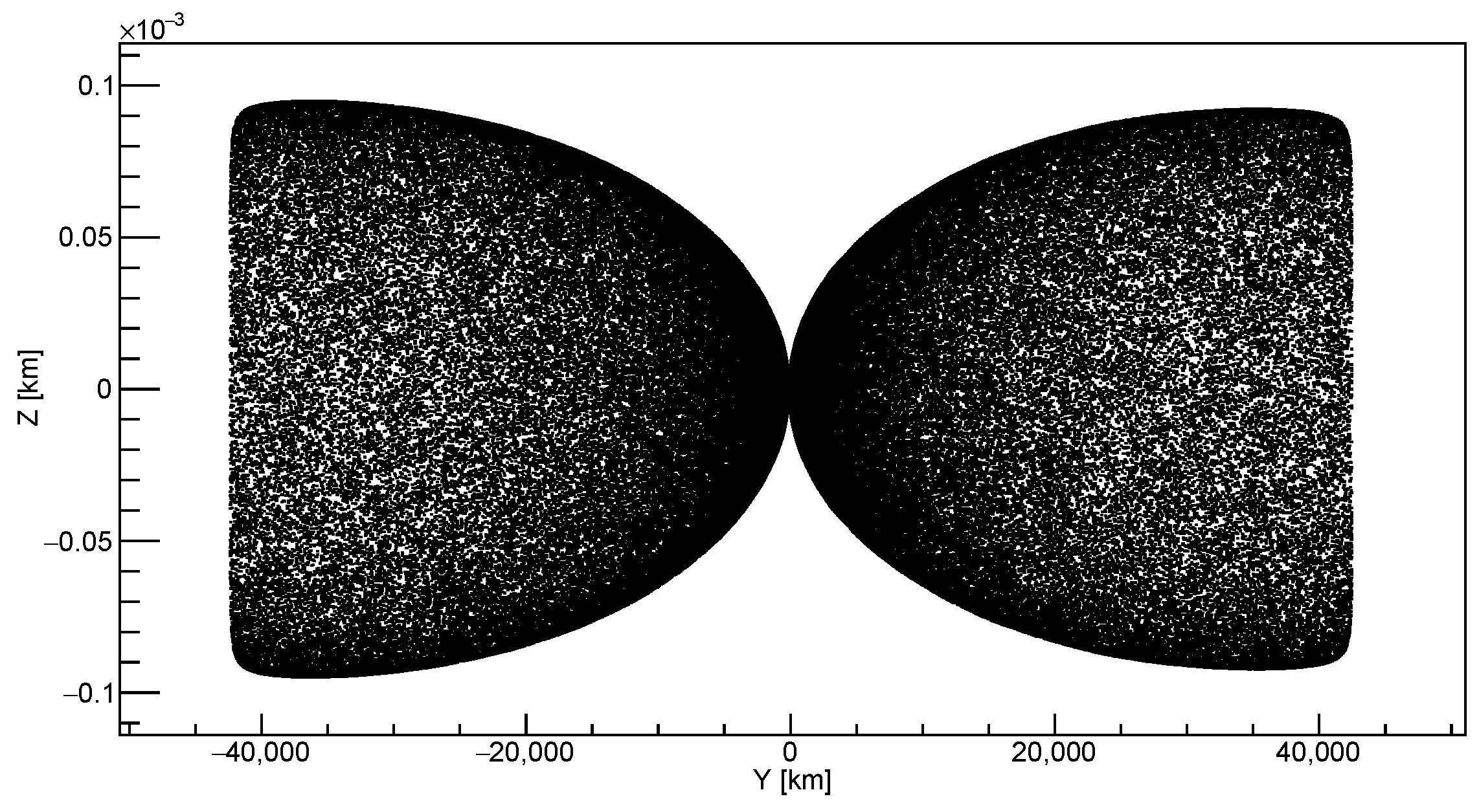
is the Lorentz factor. The azimuthal angle of emitted photon direction is random, consistent with uniform distribution. Therefore, at the ultra-relativistic regime, the direction of the emitted synchrotron photon is nearly tangential to the electron or positron trajectory. In this way, synchrotron photons may reproduce the projection of a pair-member trajectory onto the atmosphere plane. For that reason the spatial distribution of secondary photons on the top of the atmosphere is expected to be a very thin curve.
The efficiency of the simulation method presented in this article is independent of the Sun magnetic field model. Here, for simplicity, we use a dipole approximation with a magnetic dipole moment equal to 6.87 × 10 32 G cm 3 , but any other could also be used, e.g., DQCS [19], as was done in Ref. [11].

3. Materials and Methods

In order to model the UHE photon cascading in the solar magnetic field, the PRESHOWER program is used in this work. In this program, interactions are modelled by Monte Carlo simulations. However, the program had to be modified to enable the time cumulative distribution of secondary photons on the top of the atmosphere. The detailed description of the PRESHOWER program is presented in [13]. Unfortunately, the article refers to the simulator of the UHE photon interaction with the geomagnetic field, so the simulator version applied in this work is different. However, this section and the indicated article provide sufficient knowledge to understand research methods.
The PRESHOWER simulator generates sample data for determined initial conditions. Simulation parameters that could be changed were the primary photon energy, the impact parameter, and the heliocentric latitude of the primary photon trajectory. Therefore, only two coordinates of the simulation starting point could be adjusted. What is more, the primary photon direction was completely determined after the choice of parameters. For these reasons, it was necessary to update the PRESHOWER simulator, with the purpose of applying the more realistic model. The introduced modifications and program functioning are described in the following sections.
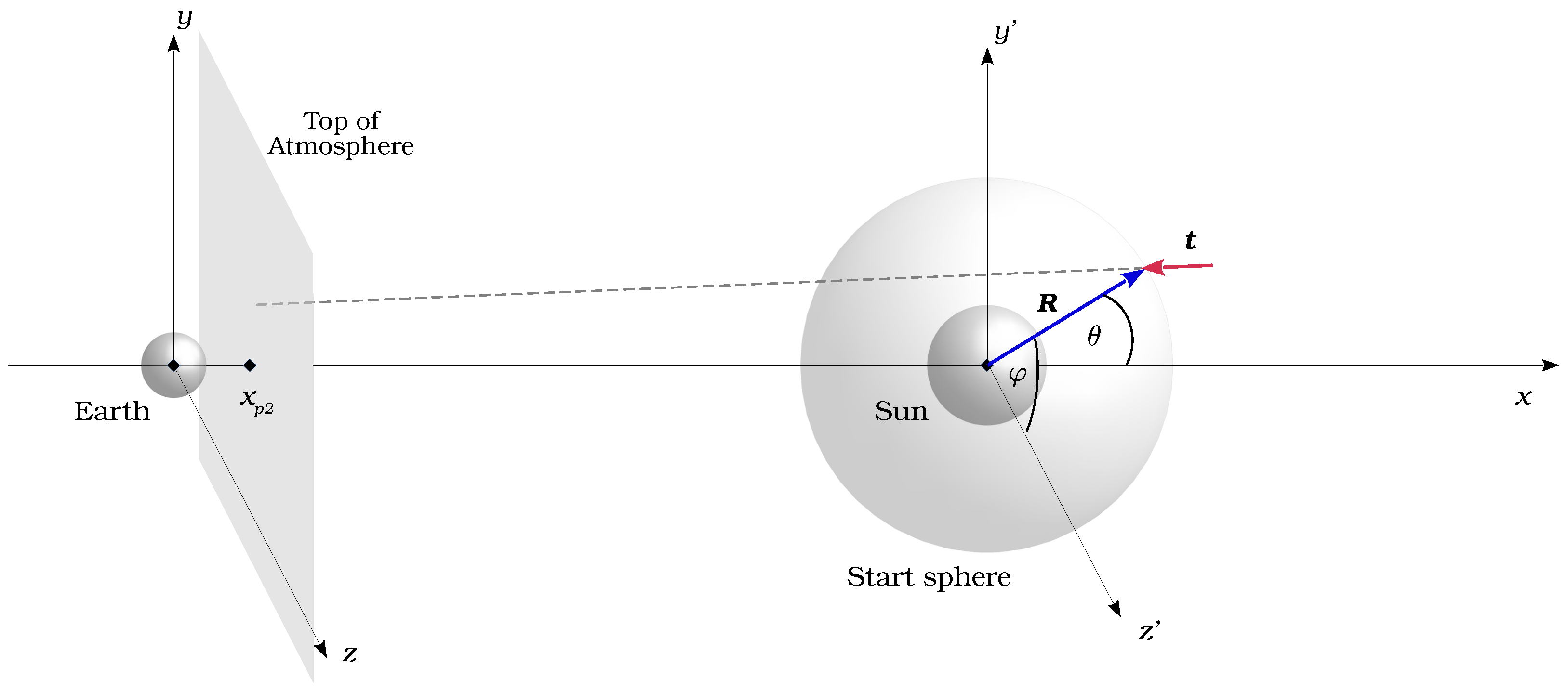
The coordinate system used in the simulator is shown in Figure 1. The applied coordinate system is similar to the heliocentric ecliptic coordinate system, but in contrast to this system, the Earth’s motion is not simulated. Therefore, the x axis is determined by the centre of the Earth and the centre of the Sun. The Earth’s centre is also the coordinate system origin. The x y plane contains the ecliptic. In fact, the simulator neglects the Earth and its atmosphere curvature. The atmosphere flat is modelled by a plane with equation x = 112.83 km. In the scheme, simulation parameters–the impact parameter and the heliocentric latitude of the primary photon trajectory—are indicated. The impact parameter in this model is the distance between the primary photon trajectory and the Sun’s centre, whereas the heliocentric latitude is defined as the angular distance between the ecliptic and a simulation starting point in the heliocentric coordinate system. In this way, the simulation starting point is completely determined because the x coordinate of the starting point is a constant value for all simulations equals to 156.9 × 10 6 km, which is implemented in the code and cannot be adjusted.
Moreover, the primary photon is always aimed at the centre of the atmosphere plane. Therefore, it is assigned after a simulation parameter choice. In this case, the heliocentric latitude remains unchangeable throughout the primary photon propagation.
For proper functioning of the program, many functions with different destinations need to be applied, among others, the CERN routine DBSKA for calculating the modified Bessel functions. The most important function of the simulator performs a loop on particles and simulates physical processes involving them and propagates them. The loop includes only the primary UHE photon and possibly the primary pair, because secondary photons’ directions are not altered and they do not need to be propagated step-wise. Thus, their position at the top of the atmosphere is calculated just after their generation and potential secondary photon cascading is neglected.
The function calculates a simulation starting point for given input parameters. Then, it propagates the UHE photon and simulates its conversion gradually. In each step, the probability for conversion is computed according to Formula (3).
For a stochastic sampling of the probability for the process occurrence, the long period pseudo-random number generator is used. Generated numbers are consistent with the uniform distribution. Therefore, thanks to imposing the condition that the process occurs if the generated number is less than the calculated probability, the simulation reflects the probability distribution for the considered process. When the electron-positron pair is created, the fractional energy is simulated similarly to the conversion probability, with respect to its probability distribution (4).
Then, the electron and positron are propagated step-wise according to Formula (5). The distance Δ s chosen in each step, which refers to the time interval Δ t , depends on the magnetic field strength for the particle location in space and the current particle energy. Secondary photon emission is simulated by analogy with the primary photon conversion. The probability for this process is computed on the basis of Formula (6). The approximation (7) is adopted as the angle of synchrotron photon deflection from the electron or positron trajectory. In turn, the angle of photon direction in the plane horizontal to the emitting particle trajectory is sampled from the uniform distribution. The simulation ends when the primary photon or the created particles reach the top of the atmosphere. All obtained particle data are stored in a matrix, which has a fixed size. Therefore, the maximum number of particles generated in the simulation is limited.
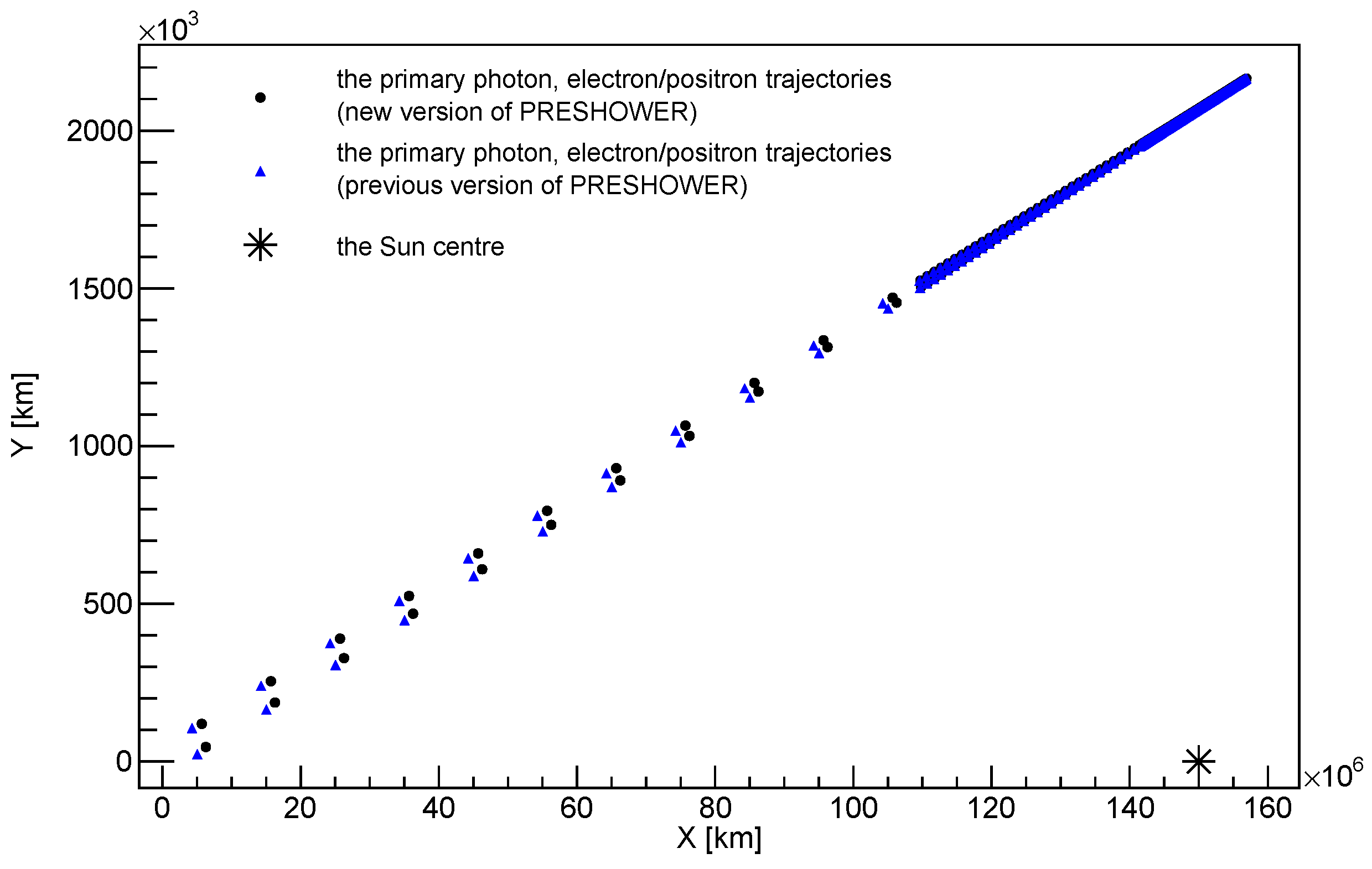
On the basis of the simulation results, the spatial distribution of secondary photons at the top of the atmosphere may be analysed in detail in the case of the UHE photon aimed at the top of the atmosphere. The influence of simulation input parameters on the distribution of secondary photons at the top of the atmosphere was the subject of a previous study [11].
Previous results indicated that it is justified to consider a more realistic case, in which UHE photons reaching the Sun’s vicinity from every direction are modelled. Furthermore, it was assumed that the UHE photon flux is isotropic. Nevertheless, this approach required substantial changes in the program’s functioning.
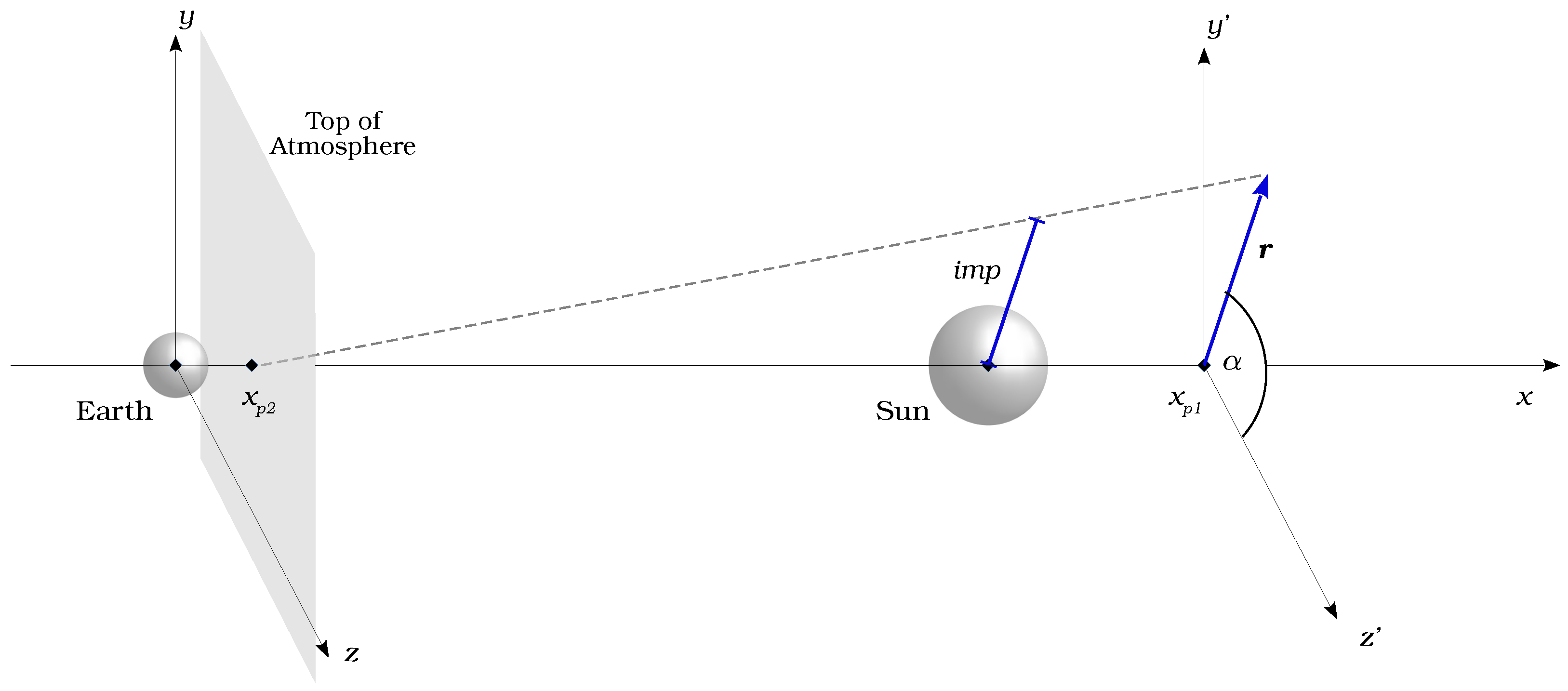
The most crucial modification concerned the arbitrary direction of the UHE photon, which implies the need for new simulation parameters and a new method of calculating the simulation starting point. On the basis of assumptions made about the UHE photon flux, it was found that the most suitable for simulations is the heliocentric coordinate system. Figure 2 illustrates the modified coordinate system. It is worth mentioning that the inclination angle θ in the coordinate system is defined as an angle between the x axis and the position vector.
In the new version of PRESHOWER, simulation starting points should be isotropically distributed at the sphere surface. Therefore, the radius of this starting sphere was chosen as the simulation parameter, whereas the position on the starting sphere is generated in such a way that every solid angle is equally probable. This condition may be described as
d N d Ω = const C ,
where d N is the number of UHE photons at the starting sphere in the solid angle d Ω . Therefore, the probability of generating the primary photon at the position with the azimuthal angle from interval [ φ , φ + d φ ] should be equal to
P φ = 1 N Ω 0 d N d Ω d Ω = 1 N 0 π sin θ d θ φ φ + d φ C d φ = C N d φ ,
where N is the total number of UHE photons reaching the starting sphere. The probability density function of the azimuthal angles is constant
f ( φ ) = d P φ d φ = C N = const
and the variable is described by the uniform distribution. Similarly, one may obtain that
f ( cos θ ) = const
and cos θ is uniformly distributed. Therefore, in the applied function φ and cos θ are randomly generated from uniform distribution and then the simulation starting point is calculated using the standard transformation between spherical coordinates and Cartesian coordinates. In the transformation, the redefinitions of the θ angle and the Sun’s position are included. The isotropic primary photon direction is modelled analogically. Nevertheless, the transformations from ( θ ˜ , φ ˜ ) coordinates to coordinates used in the simulation are more complex. Due to the fact that ( θ ˜ , φ ˜ ) are defined in the local coordinate system related to the position on the starting sphere, generated angles are firstly transformed to the local Cartesian system
e ^ x ˜ = sin θ cos φ , e ^ y ˜ = sin θ sin φ , e ^ z ˜ = cos θ .
The minus sign results from considering primary photons coming from the outside of the starting sphere. The local versors may be identified as spherical versors
e ^ z ˜ = e ^ r , e ^ x ˜ = e ^ θ , e ^ y ˜ = e ^ ϕ
related to the position on the starting sphere ( θ S , φ S ) . Therefore, they are expressed in coordinates used in the simulator (Figure 1) using formulas
e ^ x = e ^ z ˜ cos θ S e ^ x ˜ sin θ S e ^ y = e ^ z ˜ sin θ S cos φ S e ^ y ˜ sin φ S + e ^ x ˜ cos θ S cos φ S e ^ z = e ^ y ˜ cos φ S + e ^ x ˜ cos θ S sin φ S + e ^ z ˜ sin θ S sin φ S .
Additionally, the drawn value cos θ ˜ belongs to the interval [ 0 , 1 ] since we consider only the range of polar angles [ 0 , π / 2 ] , which responds to directions beneath the sphere surface.
The generalisation of the program for an arbitrary primary photon direction required also changes in the simulation end condition. The previous condition may be effectively applied only to primary photons aimed at the atmosphere plane. Thus, assuming the plane is infinite, the previous condition is placed on photons with the negative component of the direction versor. In other cases, the simulation end condition is the distance to the Sun’s centre larger than 7 R . What is more, the propagation of the primary photon, electron, or positron is aborted in case the particle lands on the Sun. In turn, secondary photons aimed at the Sun are not even included in the particle table. In the previous version of the program, these additional conditions were not needed, because of the specific determination of the primary photon direction. This approach enables considering also the potential special cases of the UHE photon cascading. For instance, it takes into account the primary photons not aimed at the Earth that may generate observable secondary photons after conversion thanks to the change of electron or positron direction in the magnetic field.

4. Results

Introduced amendments allowed simulation of the cumulative distribution of secondary photons at the top of the atmosphere. However, the new version of the simulator needed to be verified in detail beforehand. Therefore, both the validation of the simulator and the preliminary analysis of the results are described in the following sections.

4.1. Verification of the PRESHOWER Functioning

It was significant to analyse simulation results firstly with respect to the correctness. This verification was performed both for appended functions and for the simulation as a whole. In the case of added functions, we visualised their results separately and compared them with expected outcomes. For this purpose, we analysed the distribution of solid angles generated without performing complete simulations and then visualised calculated positions at the sphere and directions. On the basis of 100,000 generated cos θ and φ values, it was found that the distribution of solid angles is flat. Similarly, the visualisations of position and direction distributions were in line with our expectations. With the purpose of verifying the whole program and the interoperability of its functions, it was necessary to compare results from the present version of the PRESHOWER with those from the previous version. However, this comparison should concern an identical physical event. Therefore, the simulation starting point, the primary photon direction, and the energy must be the same in both used simulator versions. We considered the case when the primary photon with energy 100 EeV aimed at the Earth propagates in the Sun’s vicinity with the impact parameter 3 R and the heliocentric latitude 0 . This responds to the following parameters in the current PRESHOWER version: the simulation starting point ( R , θ S , ϕ S ) = ( 10.44 R , 0.29 , 0 ) , where R is the starting sphere radius, and the primary photon direction ( θ ˜ , ϕ ˜ ) = ( 0.28 , π ) . In this simple case, the primary photon, electron, and positron are propagating only in the x y plane. Their movement modelled by both simulations is illustrated in Figure 3. The graph shows particle positions for each thousandth step of the simulation.
It was found that the propagation of particles is similar in both cases. Minor differences such as distances between the next steps are caused by a different conversion point. This, in turn, results from the stochastic nature of physical processes. Furthermore, the distribution of secondary photons at the top of the atmosphere is presented in Figure 4. The generated distribution has a line-like shape and a size 8.48 × 10 4 km, which is a reasonable outcome. In accordance with previous results [11], the distribution size for chosen input parameters should be approximately 10 5 km.
Therefore, obtained results are correct and it was concluded that the simulator properly models UHE photon cascading.

4.2. Optimisation of the Simulation

The inclusion of more cases in the simulation, unfortunately, extended the computation time. It was found that the simulator needs to be optimised. Due to this fact, we reduced the cases included by the program and adjusted its parameters.

4.2.1. Reducing Considered Cases

The first simulations showed that only a few of them gave rise to observable effects on the Earth. Thus, most of the calculation time was used for cases that are not the subject of this study. With the purpose of effective use of computer resources, we refrained from modelling the special cases of the UHE photon cascading. Additional conditions were placed on the primary photon direction and its arrival point at the top of the atmosphere. Only primary photons moving towards the negative x axis are simulated. In turn, the primary photon arrival point is usually related to the centre of secondary photons distribution. In this way, limiting its distance from the x axis (Figure 2) increases the probability of the observation on the Earth. The limit on the distance between the point at the top of the Earth’s atmosphere where the UHE photon would have landed if no conversion had occurred, and the x axis connecting the Earth’s and the Sun’s centres is hereinafter referred to as the arrival point limit. Conditions are checked at the beginning of the program and further procedures are performed only for primary photons that fulfil limits. What is more, the number of secondary photons saved to the outfiles was limited to particles that are not further than 6500 km from the x axis at the top of the atmosphere.

4.2.2. Adjustment of Simulation Parameters

The implemented limit on the centre of the secondary photons spatial distribution and the starting sphere radius—the simulation input parameter—should also be adjusted for the optimisation of the simulation. The limit on the primary photon arrival point has an influence on the ratio of events observable on the Earth to all simulations that fulfilled the condition. The number of simulations giving observable effects increases with the decrease in the distance from the x axis to the centre of the secondary photons signature. On the other hand, the limit obviously affects the fraction of simulations that fulfil the condition and in this way the computation time. The strengthening of the limit on the primary photon arrival point results in a decline in the ratio of simulation fulfilling the condition for all running simulations and considerably prolongs the calculation time. These relations are shown in Figure 5 and Figure 6.
On the basis of the obtained data, we calculated the ratio of events observable on the Earth to all running simulations, which is illustrated in Figure 7. It was observed that the fraction of detectable events is greater for the relaxation of the condition. However, the statistics for this range are based on few entries, so it may be burdened with high risk.
Figure 5 shows that the number of simulations fulfilling the condition depends weakly on the starting sphere radius. Thus, the fraction of simulations observed on the Earth was calculated only for the starting sphere radius 6 R (Figure 6). In order to consider the largest number of events observable on the Earth in a relatively short time, the arrival point limit was set at 10 4 km. The number of CRE effects in all effects detectable on the Earth, in turn, is dependent on the starting sphere radius. Due to the fact that the starting sphere radius has an influence on impact parameters of primary photons, it also affects the probability of their conversion. On the other hand, the decrease in the starting sphere radius may also eliminate some cases that can give observable effects at the top of the atmosphere. Therefore the starting sphere radius 6 R was chosen as an optimum value for the simulation parameter. The resulting preliminary cumulative distribution of secondary photons at the top of the atmosphere is shown in Figure 8. The results were obtained only for the primary photons of energy 100 EeV. However, the presented method may be applied to the whole energy spectrum of UHE photons.
We enlarged the considered observable area to take into account the cross section of the Earth and the surrounding atmosphere. The distribution includes 324 CRE effect signatures, which corresponds to one year of observation taking into account present limits on the UHE photon flux [14]. However, the presented distribution does not include cases reduced due to the calculation time and technical limitations of detectors. Hence, the number of predicted CRE effect signatures per year may be fraught with great uncertainty. Observed line-like signatures are parts of large cascades with centres beyond the Earth’s cross-section. Due to the fact that cascades are produced by UHE photons in the vicinity of the Sun, many secondary photons have directions contained in the solid angle determined by the Sun. Therefore, CRE effect cascades should distinguish themselves from the rest of the observations since secondary photons may reach higher energies than photons emitted by the Sun. The anomaly in the very-high-energy photon flux was already observed (see [20,21]). However, the UHE photon cascading was not taken into account as a possible source to date. Therefore, it is significant to analyse the cumulative distribution of secondary photons with regard to unique features that could help to classify them. The possible anisotropy may be observed in the distribution of the orientation of signatures at the top of the atmosphere. The horizontal or nearly horizontal orientation could be more frequent. It would also be theoretically motivated since signatures oriented in this way are generated by UHE photons that have a heliocentric latitude around 0 or 90 at the conversion point [1]. Simultaneously, the conversion occurs more often for the heliocentric latitude 90 [11]. In order to describe the orientation of signatures, the rotation angle parameter was introduced. It is given by the equation
α = arctan z 1 z 2 y 1 y 2 ,
where points ( y 1 , z 1 ) and ( y 2 , z 2 ) are related to secondary photons that are the farthest, but still located in the observable area. The rotation angle is in the range of ( π / 2 , π / 2 ) . The obtained distribution is shown in Figure 9.

5. Discussion

The previous study ([1,11]) showed that the UHE photon interaction with the solar magnetic field may result in the extremely extended, line-like shaped cascade of secondary photons reaching the top of the Earth’s atmosphere. Owing to the unique signature, the footprint of secondary photons at the top of the atmosphere should be possible to observe and classify. Due to the expected wide spatial span of these cascades, it should be possible to observe not only secondary photons produced by primary UHE photons aimed at the Earth, but also the tails of the secondary photons produced by primary UHE photons directed far from the Earth. In this article, we presented a successful method for modelling the interactions of the isotropic UHE photon flux with the solar magnetic field in order to obtain for the first time particle distributions containing secondary photons from both central and peripheral parts of the CRE cascades. The method is based on using the PRESHOWER program appropriately modified and optimised. We verified the functioning of the simulator and checked that obtained results are perfectly consistent with the previous analyses [11]. In order to investigate the cumulative distribution of secondary photons at the top of the atmosphere, we discussed the impact of simulation parameters on the modelled physical phenomena and found optimal values for these parameters. The results obtained in this way indicate that secondary photons produced by the UHE photons not aimed at the Earth contribute significantly to the cumulative distribution of secondary photons at the top of the atmosphere and to the distributions of CRE footprint orientations which might serve as a valuable observational hint. In relation to the methods described here, it is important to note that recent observations ([20,21]) demonstrate yet unexplained gamma-ray emission from the solar disk. In light of the simulations of CRE resulting from the interactions of UHE photons nearby the Sun, one might speculate that these observations may be a signature of the CRE effect, which motivates a dedicated analysis in this direction. We conclude that it is justified and indispensable to simulate the flux of UHE photons cascading in the Sun’s vicinity without neglecting the tails of the resultant CRE distributions, and that the presented method enables us to search for potentially observable signatures of the CRE effect, and hence offer a novel perspective for an indirect search for UHE photons. We proposed that one such signature might be seen in a distribution of the spatial orientations of the CRE cascades at the top of the atmosphere. What is more, the prepared method also allows us to estimate the flux of CRE cascades per year and quantise its increase, which could be directly compared to the anomalous gamma-ray emission from the solar disk. A quantitative evaluation of the appropriateness of proposed observables for the CRE and UHE photon searches would require a separate study, which has already been planned. Furthermore, a modified PRESHOWER program may be used along with standard simulators of the cosmic rays’ propagation to model the UHE photon conversion in the vicinity of other distant astrophysical objects. Therefore, it may also provide a new method for investigating the CRE cascades of galactic or extragalactic origin.

Author Contributions

Conceptualisation, B.P., T.B., N.D., P.H., D.A.-C.; investigation, B.P., T.B., N.D., P.H.; methodology, B.P., T.B., N.D., P.H.; software, B.P., N.D., P.H.; theoretical studies, B.P., T.B., D.A.-C.; writing—original draft preparation, B.P., T.B., N.D., P.H.; writing—review and editing, B.P., T.B., N.D., O.S., S.S., P.H., M.P., T.W., J.S., P.K., K.S., M.D.R.F., M.N., J.M., T.S., Ł.B., A.T., L.D.P., K.R.; All authors have read and agreed to the published version of the manuscript.

Funding

This research received no external funding.

Institutional Review Board Statement

Not applicable.

Informed Consent Statement

Not applicable.

Data Availability Statement

The data presented in this study are results of the simulations and are reproducible. The simulator code is available on request from the corresponding author. The simulator code is not publicly available due to its storage on ACC Cyfronet AGH-UST servers.

Acknowledgments

This research was supported in part by PLGrid Infrastructure.

Conflicts of Interest

The authors declare no conflict of interest.

Abbreviations

The following abbreviations are used in this manuscript:
UHEUltra-High Energy
CRECosmic Ray Ensembles
EASExtensive Air Shower
CREDOCosmic-Ray Extremely Distributed Observatory

References

  1. Homola, P.; Beznosko, D.; Bhatta, G.; Bibrzycki, Ł.; Borczyńska, M.; Bratek, Ł.; Budnev, N.; Burakowski, D.; Alvarez-Castillo, D.E.; Almeida Cheminant, K.; et al. Cosmic-Ray Extremely Distributed Observatory. Symmetry 2020, 12, 1835. [Google Scholar] [CrossRef]
  2. Greisen, K. End to the cosmic ray spectrum? Phys. Rev. Lett. 1966, 16, 748. [Google Scholar] [CrossRef]
  3. Zatsepin, G.T.; Kuzmin, V.A. Upper limit of the spectrum of cosmic rays. JETP Lett. 1966, 4, 78. [Google Scholar]
  4. Yao, W.M.; Amsler, C.; Asner, D.; Barnett, R.M.; Beringer, J.; Burchat, P.R.; Carone, C.D.; Caso, C.; Dahl, O.; D’Ambrosio, G.; et al. Review of Particle Physics. J. Phys. G Nucl. Part. Phys. 2020, 33, 083C01. [Google Scholar] [CrossRef]
  5. Kuzmin, V.; Rubakov, V. Ultrahigh-energy cosmic rays: A window on postinflationary reheating epoch of the Universe? Phys. At. Nucl. 1998, 61, 1028–1030. [Google Scholar]
  6. Birkel, M.; Sarkar, S. Extremely high energy cosmic rays from relic particle decays. Astropart. Phys. 1998, 9, 297–309. [Google Scholar] [CrossRef]
  7. Frampton, P.H.; Keszthelyi, B.; Ng, Y.J. Longevity and Highest-Energy Cosmic Rays. Int. J. Mod. Phys. D 1999, 8, 117–122. [Google Scholar] [CrossRef]
  8. Blasi, P.; Dick, R.; Kolb, E.W. Ultra-high energy cosmic rays from annihilation of superheavy dark matter. Astropart. Phys. 2002, 18, 57–66. [Google Scholar] [CrossRef]
  9. CREDO Detector. Available online: https://credo.science/#/detector/tutorial (accessed on 16 May 2022).
  10. Bibrzycki, Ł.; Burakowski, D.; Homola, P.; Piekarczyk, M.; Niedźwiecki, M.; Rzecki, K.; Stuglik, S.; Tursunov, A.; Hnatyk, B.; Castillo, D.E.A.; et al. Towards A Global Cosmic Ray Sensor Network: CREDO Detector as the First Open-Source Mobile Application Enabling Detection of Penetrating Radiation. Symmetry 2020, 12, 1802. [Google Scholar] [CrossRef]
  11. Dhital, N.; Homola, P.; Alvarez-Castillo, D.; Góra, D.; Wilczyński, H.; Almeida Cheminant, K.; Poncyljusz, B.; Mędrala, J.; Opiła, G. Cosmic ray ensembles as signatures of ultra-high energy photons interacting with the solar magnetic field. J. Cosmol. Astropart. Phys. 2022, 2022, 038. [Google Scholar] [CrossRef]
  12. Homola, P.; Góra, D.; Heck, D.; Klages, H.; Pękala, J.; Risse, M.; Wilczyńska, B.; Wilczyński, H. Simulation of ultra-high energy photon propagation in the geomagnetic field. Comput. Phys. Commun. 2005, 173, 71–90. [Google Scholar] [CrossRef]
  13. Homola, P.; Engel, R.; Pysz, A.; Wilczyński, H. Simulation of ultra-high energy photon propagation with PRESHOWER 2.0. Comput. Phys. Commun. 2013, 184, 1468–1475. [Google Scholar] [CrossRef]
  14. Rautenberg, J. Limits on ultra-high energy photons with the Pierre Auger Observatory. In Proceedings of the 36th International Cosmic Ray Conference (ICRC2019), Madison, WI, USA, 24 July–1 August 2019; p. 398. [Google Scholar] [CrossRef]
  15. Erber, T. High-Energy Electromagnetic Conversion Processes in Intense Magnetic Fields. Rev. Mod. Phys. 1966, 38, 626–659. [Google Scholar] [CrossRef]
  16. Daugherty, J.; Harding, A. Pair production in superstrong magnetic fields. ApJ 1983, 273, 761–773. [Google Scholar] [CrossRef]
  17. Sokolov, A.; Ternov, I.; Kilmister, C.; Chomet, S. Radiation from Relativistic Electrons; AIP Translation Series; AIP: New York, NY, USA, 1986. [Google Scholar]
  18. Wiedemann, H. Synchrotron Radiation. In Advanced Texts in Physics; Springer: Berlin, Germany, 2003. [Google Scholar]
  19. Banaszkiewicz, M.; Axford, W.; Mckenzie, J. An analytic solar magnetic field model. Astron. Astrophys. 1998, 337, 940–944. [Google Scholar]
  20. Albert, A.; Alfaro, R.; Alvarez, C.; Arceo, R.; Arteaga-Velázquez, J.C.; Rojas, D.A.; Solares, H.A.; Belmont-Moreno, E.; BenZvi, S.Y.; Brisbois, C.; et al. First HAWC observations of the Sun constrain steady TeV gamma-ray emission. Phys. Rev. D 2018, 98, 123011. [Google Scholar] [CrossRef]
  21. Rainó, S.; Giglietto, N.; Moskalenko, I.; Orlando, E.; Strong, A. Fermi Large Area Telescope Observations of the gamma-ray emission from the Quiescent Sun. Nucl. Part. Phys. Proc. 2017, 291–293, 36–39. [Google Scholar] [CrossRef]
Figure 1. The coordinate system used in the previous version of the PRESHOWER simulator. The dashed line shows the primary photon trajectory, x p 1 —the fixed x coordinate of the simulation starting point; the distance between x p 1 and the Sun’s centre is 10 R . The i m p (blue line) is the impact parameter (the input simulation parameter) and the blue vector r , which lies in the y z plane, points at the simulation starting point. The angle α between the r and the z axis is the heliocentric latitude (the simulation input parameter), while the vector length | r | = r _ a t _ b e g i n n i n g is a parameter calculated during the simulation. The x p 2 point determines the top of the atmosphere plane x = x p 2 and it is the arrival point of the primary photon.
Universe 08 00498 g001
Figure 2. The coordinate system used in the modified version of the PRESHOWER simulator. The dashed line shows the primary photon trajectory. The purple vector t is the primary photon direction, which is randomly generated. The blue vector R indicates the simulation starting point; its length R is the simulation input parameter, whereas the polar angle θ between the vector R and the x axis and the azimuthal angle φ in the y z plane is randomly generated. The x p 2 point determines the top of the atmosphere plane x = x p 2 , but it is no longer the primary photon arrival point.
Universe 08 00498 g002
Figure 3. Comparison of particle (the primary photon and the positron–electron pair) propagation in the previous and modified version of PRESHOWER, for the exemplary simulation with the primary photon energy 100 EeV.
Universe 08 00498 g003
Figure 4. The spatial distribution of secondary photons at the top of the atmosphere produced in the exemplary simulation from Figure 3. Note the difference in the scales along the y and z axes.
Universe 08 00498 g004
Figure 5. The graph of the number of simulations that fulfilled the arrival point limit in 10 10 simulations, executed for each limit, as a function of the arrival point limit, for different starting sphere radiuses: 5 R , 6 R , and 7 R .
Universe 08 00498 g005
Figure 6. The graph of the fraction of simulations, for which at least some secondary photons reached the Earth’s atmosphere, in all simulations that fulfilled the arrival point limit.
Universe 08 00498 g006
Figure 7. The calculated number of simulations giving observable effects in all executed simulations ( 10 10 ) as a function of the arrival point limit, on the basis of Figure 5 and Figure 6.
Universe 08 00498 g007
Figure 8. The cumulative spatial distribution of secondary photons at the top of the atmosphere, for the primary photon energy 100 EeV, based on 324 observable secondary photon cascades, which corresponds to one year of observation.
Universe 08 00498 g008
Figure 9. The distribution of the orientation of CRE signatures at the top of the atmosphere, for the primary photon energy 100 EeV, based on 324 CRE signatures. Histograms are normalised and divided into 100 bins.
Universe 08 00498 g009
Publisher’s Note: MDPI stays neutral with regard to jurisdictional claims in published maps and institutional affiliations.

