Abstract
As an important index of solar activity, the 10.7-cm solar radio flux (F10.7) can indicate changes in the solar EUV radiation, which plays an important role in the relationship between the Sun and the Earth. Therefore, it is valuable to study and forecast F10.7. In this study, the long short-term memory (LSTM) method in machine learning is used to predict the daily value of F10.7. The F10.7 series from 1947 to 2019 are used. Among them, the data during 1947–1995 are adopted as the training dataset, and the data during 1996–2019 (solar cycles 23 and 24) are adopted as the test dataset. The fourfold cross validation method is used to group the training set for multiple validations. We find that the root mean square error (RMSE) of the prediction results is only 6.20~6.35 sfu, and the correlation coefficient (R) is as high as 0.9883~0.9889. The overall prediction accuracy of the LSTM method is equivalent to those of the widely used autoregressive (AR) and backpropagation neural network (BP) models. Especially for 2-day and 3-day forecasts, the LSTM model is slightly better. All this demonstrates the potentiality of the LSTM method in the real-time forecasting of F10.7 in future.
1. Introduction
The term “space weather” appeared in the early 1980s and became popular in the 1990s. Space weather, as defined by Wright et al. [1], refers to the comprehensive situation of changing material conditions on the surface of the Sun, the Sun–Earth space, the Earth’s magnetic field, and the upper atmosphere that can affect the performance and reliability of the space-based and ground-based technology system and endanger human health and life. To be brief, space weather refers to how solar activity has an unwanted impact on technical systems and human activities, both in near-Earth space and on the ground. Space weather events will also cause threats and harm to human life, such as communications, navigation and positioning systems, aerospace safety, and so on. Therefore, it is necessary to carry out space weather research, including global space weather monitoring and forecasting, which is one of the guarantees for the safe operation of important national infrastructure and is closely related to us.
Solar activity controls the changes in the solar–terrestrial space environment and the space environment near the Earth, and it is the source of various geophysical phenomena and space environmental effects. Therefore, predicting the level of solar activity is an important part of space environmental forecasting. Great progress has been made in solar activity forecasting during the past few decades (see Daglis et al. [2]).
The solar radio flux of 10.7 cm (2800 MHz), commonly known as the F10.7 index, is a good indicator of solar activity. It is one of the solar indices with the longest observational record. F10.7 is closely related to the number of sunspots and some ultraviolet (UV) and visible solar irradiance records [3,4]. Since 1947, F10.7 has been measured in Canada, first at Ottawa, Ontario and then at the Penticton Radio Observatory in British Columbia, Canada (COVINGTON 1947). Unlike other solar indices, F10.7 radio flux can be easily and reliably measured from the Earth’s surface in all weather conditions. In addition, the orbit prediction of low Earth orbit satellites usually uses the upper atmosphere density model, which requires the input of future F10.7 [5,6,7]. Therefore, the accurate prediction of F10.7 is particularly important.
The radio emission of F10.7 comes from the high chromosphere and the low corona. It has a strong correlation with the existence of active regions and the occurrence of flares [8]. Therefore, some studies use the empirical prediction model based on the main solar characteristics to predict F10.7. For example, Wen et al. [9] used the physical parameters of the solar active regions to predict F10.7. Henney et al. [10] predicted F10.7 using advanced predictions of the global solar magnetic field generated by the flux transport model. Liu et al. [11] used two models established by Yeates et al. [12] and Worden and Harvey [13] to predict the short-term variations of F10.7 from 2003 to 2014. Ye et al. [14] proposed a forecast formula of F10.7 based on the classification of the area of the solar active region and correlations between the area of the solar active region and F10.7.
Miao et al. [15] used the method of “similar cycle” to forecast the mean value of solar F10.7 in the 23th solar cycle. Compared with the forecast result deduced indirectly from the sunspot number, the direct result obtained by the method of “similar cycle” was closer to the smoothed value of the monthly data of F10.7. Zhong et al. [16] used the singular spectrum analysis method to make a 27-day forecast of F10.7, and their results showed that this method predicts the periodic changes of the F10.7 index better in terms of the solar minimum. Liu et al. [17] used the autoregressive method for time series modeling to study the medium-term forecast of the solar 10.7-cm radio flux. When solar activity is weak and F10.7 shows an obvious 27-day periodic tendency, the prediction accuracy of this method is high. However, the prediction accuracy becomes low when the solar active region appears or disappears. Based on the principle of the short-period oscillation of solar radiation, Wang et al. [18] used the historical radiation index data of 135 days to forecast F10.7 in 54 days. This method was slightly better than the method of the Space Weather Prediction Center in America, and the RMSE decreased by about 19% for the short-term forecast of 7 days. Lei et al. [19] proposed an empirical method to predict the F10.7 of 27 days based on EUV images. They defined the contribution index (PSR) of solar corona to F10.7 according to the intensity of the solar extreme ultraviolet image. Compared with the prediction result of the 54-order autoregressive model in 2012–2013, this method has obvious advantages in the prediction of F10.7 during the next 3–27 days.
Machine learning is a subfield of computer science which presents an automatic learning ability without explicit programming [20]. It evolved from the research of pattern recognition and computational learning theory in artificial intelligence. Machine learning is a method that first trains a model by data and then predicts future data by the trained model. In the past 10 years, machine learning has been a concern in a wide range of fields with the development of computer hardware. It is particularly suitable for big data and multi-dimensional data processing. It has also been used more and more in space weather research, especially for the prediction of spatial environmental parameters such as F10.7. Huang et al. [21] used the support vector regression method to forecast F10.7 several days in advance. Warren et al. [22] proposed a simple linear prediction model of F10.7, and Wang et al. [23] proposed a linear multi-step F10.7 forecasting model based on task correlation and heteroscedasticity.
The neural network is an important example of machine learning technology. More and more scholars apply it to the forecasting of F10.7. For instance, Chatterjee [24] used a multi-layer feedforward neural network to predict F10.7 in 1993 (the minimum of the 22th solar cycle), which was more accurate for the prediction of 1 day in advance. The results showed that the correlation coefficient between the predicted and observed values (1 day in advance) was 0.93. Xiao et al. [25] used the backpropagation neural network technique to predict the daily F10.7. Their results showed that this method is superior to other forecasting methods such as support vector regression in short-term predictions. Wang [26] proposed a multi-layer prediction model of a typical neural network to predict F10.7. Luo et al. [27] proposed a method that combined a backpropagation neural network and empirical mode decomposition to predict the daily value of F10.7 1–27 days in advance.
A neural network is a method to implement machine learning tasks. In general, neural networks can be divided into two kinds: the feedforward neural network and the feedback neural network. Neurons in the feedback neural network can not only receive signals from other neurons but also receive their own feedback signals. Compared with the feedforward neural network, the neurons in the feedback neural network have a memory function and have different states at different times. Information propagation in the feedback neural network can be one-way or two-way. A recurrent neural network (RNN) is a kind of feedback neural network which is one of the most popular data-driven methods in forecasting of time series. Although RNNs can understand short-term dependencies, they have encountered problems in capturing long-term dependencies due to the problem of gradual disappearance. The long short-term memory (LSTM) method is a machine learning algorithm suitable for processing time series data which uses storage units and thresholds to capture long-term dependencies. Recently, it has shown good performance in various fields related to big data. Based on the LSTM method, Yang et al. [28] and Luo et al. [29] conducted a mid-term forecast of the F10.7 index for the next 27 days.
Different from Yang, this paper aims at a short-term forecast of the F10.7 index. Yang et al. [28] spent a lot of time to determine the setting of parameters in their model. They trained the data as a whole, and the corresponding training set and test set were not separated. Furthermore, their model ignored the local volatility of the data during a certain period of time. This paper will combine experience with theory to quickly determine the selection of parameters. In addition, we will separate the training set from the test set and ensure that the training set has enough data to train the model. Here, the test set consists of unknown data for the mode, and will be used to evaluate the generalization ability of the model. We will also consider some detailed skills to improve the accuracy of the prediction. This paper is organized as follows. The data and the LSTM model are briefly described in Section 2. The results are presented in Section 3, followed by discussion, conclusions, and future work of Section 4.
2. Data and Methods
The daily flux of F10.7 is the radio emission from the sun at the wavelength of 10.7 cm recorded daily. The units are solar flux units (). The 10.7 cm daily solar flux data were obtained from CelesTrak (https://celestrak.com/SpaceData/SpaceWx-format.php) (accessed on 23 November 2020). The database available here comprised three values: the observed, adjusted, and Series D values (absolute values).
The observed flux values were measured by a solar radio telescope, which are controlled by the solar activity level and the Sun–Earth distance. This is mainly used to study the radio short-wave communication, the magnetic storm phenomenon, the upper atmosphere temperature, and so on [3]. The flux was measured three times per day. The measurement times were 5:00 p.m. UT, 8:00 p.m. UT (local noon), and 11:00 p.m. UT from March to October. As the measuring equipment was located in the valley and relatively high-latitude regions, it was impossible to maintain these times for the rest of the year. Therefore, the times of the flux measurements were changed to 6:00 p.m. UT, 8:00 p.m. UT (local noon), and 10:00 p.m. UT from November to February so that the sun was high enough above the horizon for good measurements.
Since the distance between the Sun and the Earth keeps changing, additional values were therefore generated to correct for changes in the Sun–Earth distance. This is called the adjusted flux (the value at 1AU). Astronomers try to match the data of the solar flux density at different frequencies with a frequency spectrum. Given a scale factor, each wavelength could be combined into a calibrated spectrum. For the solar flux of 10.7 cm, the estimated scale factor was 0.9, and [30]. In this article, we use the adjusted fluxes of F10.7.
We preprocessed the data as follows. (1) Since the data from 2004 to 2019 on the website had three values per day, we calculated the daily averages of the adjusted flux values of F10.7 for each day. (2) We integrate the calculated daily average data of F10.7 from 2004 to 2019, with the daily data directly provided by the website from 1947 to 2004. Here, we used the data of F10.7 from 1947 to 2019. Figure 1 shows the processed data. The black line represents the train dataset, and the blue line is the test dataset. They will be used separately in the following.
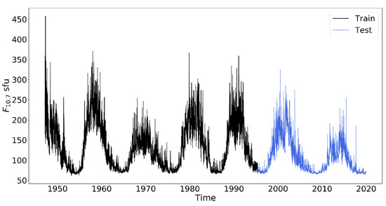
Figure 1.
Daily average of F10.7 (1AU adjusted values) from 1947 to 2019.
LSTM was introduced by Hochreiter and Schmidhuber [31] and became more and more refined and popular with the efforts of many scientists. Due to its unique design structure, LSTM is suitable for processing and predicting important events with very long intervals and delays in time series and is now widely used. Here, we apply LSTM to the prediction of F10.7.
LSTM is capable of removing or adding information to the state of the cell through a well-designed structure called a “gate”. A gate is a way of letting information through selectively. It contains a sigmoid neural network layer and a pointwise multiplication operation. The LSTM has three gates to protect and control the state of the cells, namely the forget gate, the input gate, and the output gate. The network structure diagram of LSTM is shown in Figure 2. Each black line transmits a whole vector from the output of one node to the input of other nodes. The yellow circle represents pointwise operations, such as the summing of vectors. The blue rectangle is the learned neural network layer. The combined lines represent the connection of vectors, and the separated lines represent the content being copied and then distributed to different locations.
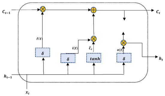
Figure 2.
The typical structure of an LSTM cell.
As the name implies, the forget gate is a gate that controls whether information is forgotten. In the framework of LSTM, it controls whether or not to forget the hidden cell state of the next layer at a certain probability. The input gate handles the input for the current sequence position, and the output gate determines what the next hidden state will be. The calculation formulas for these three gates are as follows:
where and are the coefficient and bias of the linear relationship, respectively, is the sigmoid excitation function, is the input of this time, and is the output of the cell at the previous time.
The cell input state can be found by
The update cell status can be expressed as
Finally, the output of hidden cell is obtained:
where and are the coefficient and bias of the linear relationship, respectively. The output gate and the current cell state are used to obtain the current LSTM output state , where tanh is a nonlinear activation function.
Five statistical evaluation indexes are used to evaluate the performance of the LSTM method: the mean absolute percentage error (MAPE), root mean square error (RMSE), normalized mean square error (NMSE), mean absolute error (MAE), and correlation coefficient (R). The specific formulas are as follows:
where is the number of samples, and are the predicted value and the observed value, respectively, and is the mean value of , t = 1, 2, …T.
The MAPE is the most commonly used evaluation index to express forecast errors in time series forecasting. The MAE, RMSE, and NMSE are adopted to measure the deviation between the predicted value and the observed value, which reflects the prediction performance of the model. The smaller the value is, the better the prediction will be. R is adopted to indicate the correlation between the predicted and observed values.
In this paper, the model of LSTM was established, and the calculation process was completed under the framework of Tensorflow 2.0 [32] in Python 3.7. We divided the data of 73 years into the training set and the test set. The data from 1947 to 1995 were used as the training dataset, and the data from 1996 to 2019 were used as the test dataset. The fourfold cross validation method was adopted on the training set; that is, the training set was randomly divided into a training subset and a validation subset. It was equivalent to make full use of the training set to group for multiple verifications so as to have an evaluation of the model. In the evaluation, we could adjust the parameters and select the best learner.
The parameters in the LSTM network included the learning rate and number of hidden neurons and epochs. Table 1 lists the parameters involved in the LSTM network.

Table 1.
Parameters in the LSTM model.
The Adam optimizer was chosen because of its high computational efficiency and low memory requirements [33]. The Adam optimizer is very suitable for problems with large data or parameters, and the learning rate is usually recommended to be 0.001. The epoch was set to be 100. The greater the number of hidden layer neurons, the better the representation ability of the model. However, the training time and memory cost also increase with the increase in hidden neurons. There are many ways to determine the number of hidden neurons, such as the method of determining the upper bound formula of the number of neurons [34] and the empirical formula method [35,36]. We referred to the methods mentioned above to determine the relatively optimal number of hidden layer neurons, and the number of hidden neurons was set to 50.
3. Results
3.1. Prediction Results
Figure 3 is the model loss of the 3-day forecast when epoch was 100. The blue line and yellow line represent the training set and validation set, respectively. The stability of the model loss demonstrates the effectiveness and rationality of the epoch selection.
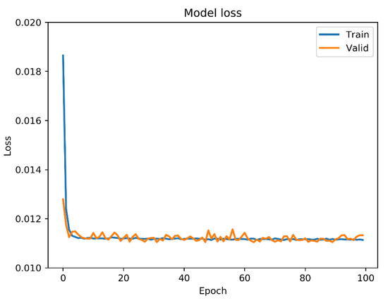
Figure 3.
The training model loss plotted along the epochs.
We used the LSTM model to predict the 1-, 2-, and 3-day values of F10.7 and compared them with the observed values. The LSTM modeling results of the 10.7-cm solar radio flux are shown in Figure 4, Figure 5 and Figure 6, which represent the results of the 3-day, 2-day, and 1-day forecasts, respectively. The observed values of F10.7 are represented by the red line, and the predicted values are represented by the blue line. We can see that the predicted values of F10.7 were in good agreement with the observed values of F10.7 in general.
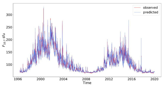
Figure 4.
Three-steps-ahead (3-day forecast) prediction of the LSTM model with the observed (red line) and predicted (blue line) F10.7 from 1996 to 2019.
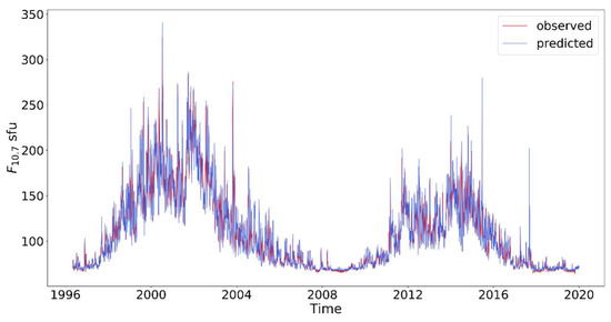
Figure 5.
The same as Figure 4 but for the two-steps-ahead (2-day forecast) prediction of LSTM.
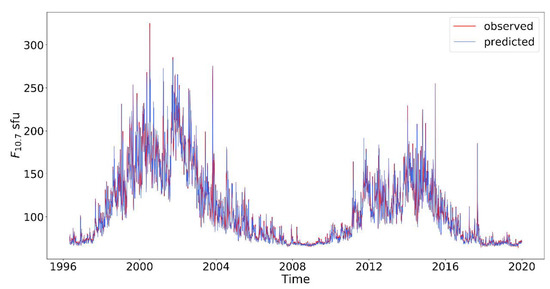
Figure 6.
The same as Figure 4 but for the one-step-ahead (1-day forecast) prediction of LSTM.
Table 2 shows the statistical parameters between the predicted and observed values of LSTM in different years, which reflects the performance of the LSTM model over time. It can be seen from Table 2 that the RMSE of LSTM roughly varied from 1 sfu to 10 sfu for the 1-day forecast. Similarly, the RMSE also ranged from 1 sfu to 10 sfu for the 2-day and 3-day forecasts, meaning that the model’s accuracy did not change significantly with the prediction’s leading time. This demonstrates the stability of the LSTM model. However, the error of the 3-day forecast had different values in different years. In order to examine the solar cycle effect of the prediction error, we conducted the following analysis.
Table 2.
The prediction errors (RMSE, MAPE, and NMSE) and R of our LSTM model for the F10.7 data during 1996–2019.
Figure 7 (left panel) displays the variations of the prediction errors by year. The yearly SSN is also shown in this figure. It can be seen from Figure 7 (left panel) that from 1996 to 2001, the error of the 3-day forecast gradually increased and reached its maximum values. Then, from 2001 to 2008, the forecast error began to decline and reached its minimum value. The prediction error changes synchronously with SSN. The variations in the 24th solar cycle presents the same pattern. Considering the fact that F10.7 also changed synchronously with the SSN (i.e., large F10.7 when the SSN is large), which means that the prediction error was large when F10.7 was large.
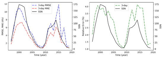
Figure 7.
Annual variations of the prediction error and SSN.
In order to eliminate the contribution of the value itself to the error, we calculated the relative error between the predicted value and the observed value. The relative prediction error was defined as
Figure 7 (right panel) shows the variations of the relative errors for the 3-day forecast. We can see that the relative error had the solar cycle effect (i.e., the relative error was large when solar activity was strong and became small when the low solar activity became weak). We need to point out that the forecast error was similar to other models even at the solar maximum years (e.g., the RMSE in 2014 of the LSTM model was 8.65 sfu, and that of the AR model was 14.51 sfu). Similar results could be found in the errors of the 1-day and 2-day forecasts.
Figure 8 displays the frequency distribution of the difference between the observed value and the predicted value of the model. Here, the differences larger than 20 sfu and less than −20 sfu are not shown in order to keep the compactness of the histogram. We see that all three predictions yielded a normal distribution of the prediction differences. The frequency was at its maximum when the difference between the observed value and the predicted value was zero, and most predictions (88% of the 3-day forecast) were located within ±5 sfu of error.
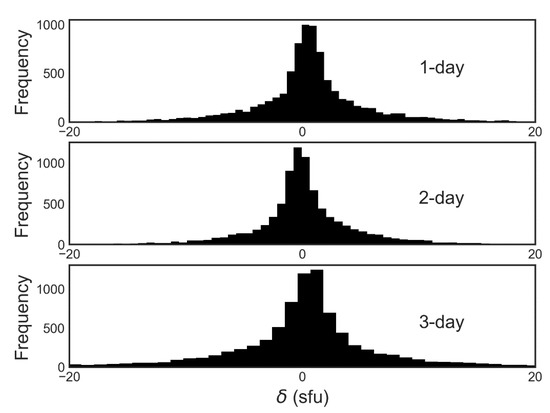
Figure 8.
The frequency distribution histogram of the difference between the observed value and the predicted value. The top, middle, and bottom panel represent the results for the 3-day, 2-day, and 1-day forecast. The abscissa represents .
3.2. Comparison with Other Models
To better evaluate the performance of the model, we compared the prediction results based on the LSTM model with those based on the AR model [37] and the BP model [25].
It can be seen from Table 3 that the 1-day forecast error of LSTM was slightly larger than that of BP. However, the LSTM model was better than the BP model for both the 2-day and 3-day forecasts. For example, the RMSE of the LSTM model was only 5.14 sfu in 2004, while that of the BP model reached 9.74 sfu.
Table 3.
Comparison of the prediction performance between LSTM and BP.
We obtained the forecast data of the AR model from 1996 to 2019. Figure 9, Figure 10 and Figure 11 show the comparison of the prediction performance between the LSTM model and the AR model. The blue column represents the prediction results of the LSTM model, and the gray one represents those of the AR model. In general, the prediction errors of the two models were both small and comparable, but they had different performances for the predictions with different leading times. For example, the performance of the AR model was slightly better (i.e., MAPE from 1.04% to 3.80%) than that of the LSTM model (MAPE from 1.04% to 4.64%) for the 1-day forecast, but they became worse for the 2-day and 3-day forecasts relative to LSTM. They could be revealed from both the prediction errors (MAPE and RMSE) and correlation coefficients. All these demonstrate that the LSTM model presented in this paper had better performance relative to the AR model, and thus the LSTM model was feasible for F10.7 prediction.
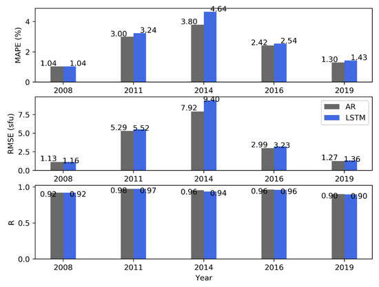
Figure 9.
Comparison of the prediction performance between the LSTM model and AR model (1-day forecast).
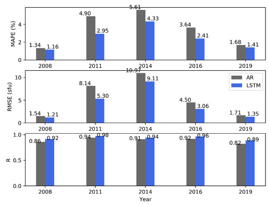
Figure 10.
The same as Figure 9 but for 2-day prediction of models.
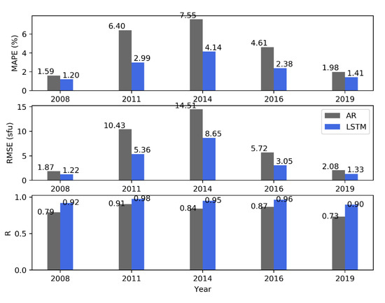
Figure 11.
The same as Figure 9 but for 3-day prediction of models.
4. Discussion, Conclusions, and Future Work
The solar radio flux of 10.7 cm (F10.7) is an important indicator of solar activity. Its use in solar physics includes the indicator of the solar activity level, a proxy of other solar emissions, the calibration data of antennas [4], the prediction of solar cycle characteristics [38], and so on. The forecast of F10.7 is an important ingredient in space weather prediction, and the accurate forecasting of F10.7 will help to protect space satellites and electricity transmission from solar radiation.
In this article, we first analyzed the ability of the LSTM model to predict the daily F10.7 during the last two solar cycles using 59 years of training samples. Secondly, we compared the prediction effects with those of the backpropagation neural network (BP) model and the autoregressive (AR) model. Our main conclusions can be summarized as follows:
- (1)
- The prediction accuracy of the LSTM model did not change significantly with the leading time of the short-term forecast (i.e., 1-day, 2-day, and 3-day forecasts). This shows the prediction stability of the LSTM model.
- (2)
- The forecast error had the solar cycle effect (i.e., larger error at the solar maximum), but even in the solar maximum year, the prediction error was still acceptable (for example, the RMSE for the 1-day forecast in 2001 was 10.19 sfu).
- (3)
- The prediction accuracy of our LSTM method was as good as those of the BP and AR models.
As the demand for space weather services increases, F10.7 daily forecasts naturally need to be improved. Thus, despite the feasibility of the LSTM method in predicting F10.7, there is still room for improvement of the predictions. This includes but is not limited to the following aspects. (1) Concerning the parameter setting of the model, in this paper, the learning rate in the LSTM network was set by an empirical formula. In the future, we can record the error after each training session by setting a different learning rate and consider the time used for training to determine the optimal learning rate. (2) For physics-based techniques and skills, in future works, we will consider some technical details to improve the forecasting effect. For example, a greater weight should be put on the samples near the test point in the model fitting, and a more scientific method will be used to find the optimal parameters and improve the model’s generalization ability. Since the LSTM model is feasible and effective to predict the solar activity index F10.7, we can explore whether the LSTM model can be applied to the forecasting and reconstruction of the number of sunspots in the future. (3) We can find from this study that the prediction errors of the 2-day and 3-day forecasts did not drop evidently. We can check the feasibility of the LSTM model in the mid-term and long-term forecasts of F10.7, which will be our next research direction.
Author Contributions
Conceptualization, W.Z. and X.Z.; methodology, W.Z., X.Z. and C.L.; software, W.Z.; formal analysis, X.F.; investigation, W.Z.; writing—original draft preparation, W.Z.; writing—review and editing, W.Z. and X.Z.; supervision, N.X., Z.L. and W.L. All authors have read and agreed to the published version of the manuscript.
Funding
This research was jointly supported by the Strategic Priority Research Program of Chinese Academy of Sciences (Grant No. XDB 41000000), NSFC grants (41531073, 41731067, 41861164026, 41874202, 41474153, and 42074183), the Youth Innovation Promotion Association of Chinese Academy of Sciences (2016133), the collaborating research program (CRP) of CAS Key Laboratory of Solar Activity NAO, and the Chinese Academy of Sciences Research Fund for Key Development Directions.
Data Availability Statement
The 10.7-cm solar flux data were obtained from the CelesTrak website (https://celestrak.com/SpaceData/SpaceWx-format.php) accessed on 23 November 2020. The SSN data used in this work were obtained from the Solar Influences Data Analysis Center (SIDC) (http://www.sidc.be/silso/datafiles) accessed on 21 January 2021.
Acknowledgments
We are grateful to Z.L. Du at NSSC CAS for providing the prediction data of the AR model.
Conflicts of Interest
The authors declare no conflict of interest.
References
- Wright, J.M., Jr.; Lennon, T.J.; Corell, R.W.; Ostenso, N.A.; Huntress, W.T., Jr.; Devine, J.F.; Crowley, P.; Harrison, J.B. The National Space Weather Program: The Strategic Plan; Office of the Federal Coordinator for Meteorological Services and Supporting Research, FCM-P30-1995: Washington, DC, USA, 1995; 18p. [Google Scholar]
- Daglis, I.A.; Chang, L.C.; Dasso, S.; Gopalswamy, N.; Khabarova, O.V.; Kilpua, E.; Lopez, R.; Marsh, D.; Matthes, K.; Nandy, D.; et al. Predictability of variable solar–terrestrial coupling. Ann. Geophys. 2021, 39, 1013–1035. [Google Scholar] [CrossRef]
- Tapping, K.F. Recent solar radio astronomy at centimeter wavelengths: The variability of the 10.7 cm flux. J. Geophys. Res. Atmos. 1987, 92, 829–838. [Google Scholar] [CrossRef]
- Tapping, K.F. The 10.7 cm solar radio flux (F10.7). Space Weather 2013, 11, 394–406. [Google Scholar] [CrossRef]
- Hedin, A.E. The atmospheric model in the region 90 to 2000 km. Adv. Space Res. 1988, 8, 9–25. [Google Scholar] [CrossRef]
- Knowles, S.H.; Picone, J.M.S.; Thonnard, E.; Nicholas, A.C. The effect of atmospheric drag on satellite orbits during the bastille day event. Solar Phys. 2001, 204, 387–397. [Google Scholar] [CrossRef]
- Picone, J.M.; Hedin, A.E.; Drob, D.P.; Aikin, A.C. NRLMSISE-00 empirical model of the atmosphere: Statistical comparisons and scientific issues. J. Geophys. Res. Space Phys. 2002, 107, SIA 15-1–SIA 15-16. [Google Scholar] [CrossRef]
- Selhorst, C.L.; Costa, J.E.; de Castro, C.G.G.; Valio, A.; Pacini, A.A.; Shibasaki, K. The 17 GHz active region number. Astrophys. J. 2014, 790, 134. [Google Scholar] [CrossRef] [Green Version]
- Wen, J.; Zhong, Q.; Liu, S. Modeling Research of 10.7 cm Solar Radio Flux 27-day Forecast of (II). Chin. J. Space Sci. 2010, 30, 198–204. [Google Scholar]
- Henney, C.J.; Toussaint, W.A.; White, S.M.; Arge, C.N. Forecasting F10.7 with solar magnetic flux transport modeling. Space Weather 2012, 10. [Google Scholar] [CrossRef]
- Liu, C.; Zhao, X.; Chen, T.; Li, H. Predicting short-term F10.7 with transport models. Astrophys. Space Sci. 2018, 363, 266. [Google Scholar] [CrossRef]
- Yeates, A.R.; Mackay, D.H.; van Ballegooijen, A.A. Modelling the Global Solar Corona: Filament Chirality Observations and Surface Simulations. Solar Phys. 2007, 245, 87–107. [Google Scholar] [CrossRef] [Green Version]
- Worden, J.; Harvey, J. An Evolving Synoptic Magnetic Flux map and Implications for the Distribution of Photospheric Magnetic Flux. Solar Phys. 2000, 195, 247–268. [Google Scholar] [CrossRef]
- Ye, Q.; Song, Q.; Xue, B. F10.7 index forecasting method based on area statistics of solar active regions (in Chinese). Chin. J. Space Sci. 2019, 39, 582–590. [Google Scholar]
- Miao, J.; Liu, S.; Xue, B.; Gong, J. Primary research on predication method of 10.7cm solar radio flux. Chin. J. Space Sci. 2003, 1, 50–54. [Google Scholar]
- Zhong, Q.; Liu, S.; He, X.; Gong, J. Application of singular spectrum analysis to solar 10.7 cm radio flux 27-day forecast. Chin. J. Space Sci. 2005, 25, 199–204. [Google Scholar]
- Liu, S.; Zhong, Q.; Wen, J.; Duo, X. Modeling Research of the 27-day Forecast of 10.7 cm Solar Radio Flux (I). Chin. Astron. Astrophys. 2010, 34, 305–315. [Google Scholar]
- Wang, H.; Xiong, J.; Zhao, C. The Mid-term Forecast Method of Solar Radiation Index F10.7. Acta Astron. Sinica 2014, 55, 302–312. [Google Scholar]
- Lei, L.; Zhong, Q.; Wang, J.; Shi, L.; Liu, S. The Mid-Term Forecast Method of F10.7 Based on Extreme Ultraviolet Images. Adv. Astron. 2019, 2019, 5604092. [Google Scholar] [CrossRef] [Green Version]
- Samuel, A.L. Some studies in machine learning using the game of checkers. IBM J. Res. Dev. 1959, 3, 211–229. [Google Scholar] [CrossRef]
- Huang, C.; Liu, D. Forecast daily indices of solar activity, F10.7, using support vector regression method. Res. Astron. Astrophys. 2009, 9, 694–702. [Google Scholar] [CrossRef] [Green Version]
- Warren, H.P.; Emmert, J.T.; Crump, N.A. Linear forecasting of the F10.7 proxy for solar activity. Space Weather 2017, 15, 1039–1051. [Google Scholar] [CrossRef]
- Wang, Z.; Hu, Q.; Zhong, Q.; Wang, Y. Linear multistep F10.7 forecasting based on task correlation and heteroscedasticity. Earth Space Sci. 2018, 5, 863–874. [Google Scholar] [CrossRef]
- Chatterjee, T.N. On the application of information theory to the optimum state-space reconstruction of the short-term solar radio flux (10.7 cm), and its prediction via a neural network. MNRAS 2001, 323, 101–108. [Google Scholar] [CrossRef]
- Xiao, C.; Cheng, G.; Zhang, H.; Rong, Z.; Shen, C.; Zhang, B.; Hu, H. Using Back Propagation Neural Network Method to Forecast Daily Indices of Solar Activity F10.7. Chin. J. Space Sci. 2017, 37, 1–7. [Google Scholar]
- Wang, X. Deep learning for mid-term forecast of daily index of solar 10.7 cm radio flux. J. Spacecr. TT C Technol. 2017, 36, 118–122. [Google Scholar]
- Luo, J.; Zhu, H.; Yu, J.; Yang, J.; Yu, H. The 10.7-cm radio flux multistep forecasting based on empirical mode decomposition and back propagation neural network. IEEJ Trans. Electr. Electron. Eng. 2020, 15, 584–592. [Google Scholar] [CrossRef]
- Yang, X.; Zhu, Y.; Yang, S.; Wang, X.; Zhong, Q. Application of LSTM neural network in F10.7 solar radio flux mid-term forecast (in Chinese). Chin. J. Space Sci. 2020, 40, 176–185. [Google Scholar]
- Luo, J.; Zhu, L.; Zhu, H.; Chien, W.; Liang, J. A New Approach for the 10.7-cm Solar Radio Flux Forecasting: Based on Empirical Mode Decomposition and LSTM. Int. J. Comput. Intell. Syst. 2021, 14, 1742–1752. [Google Scholar] [CrossRef]
- Tanaka, H.; Castelli, J.P.; Covington, A.E. Absolute calibration of solar radio flux density in the microwave region. Solar Physics 1973, 29, 243–262. [Google Scholar] [CrossRef]
- Hochreiter, S.; Schmidhuber, J. Long Short-Term Memory. Neural Comput. 1997, 9, 1735–1780. [Google Scholar] [CrossRef]
- Singh, P.; Manure, A. Introduction to TensorFlow 2.0. In Learn TensorFlow 2.0; Springer Apress: Berkeley, CA, USA, 2020; Chapter 1; pp. 1–24. [Google Scholar]
- Kingma, D.P.; Ba, J.L. Adam: A method for stochastic optimization. arXiv 2015, arXiv:1412.6980v9. [Google Scholar]
- Jadid, M.N.; Fairbairn, D.R. The application of neural network techniques to structural analysis by implementing an adaptive finite-element mesh generation. Artif. Intell. Eng. Design Anal. Manuf. 1994, 8, 177–191. [Google Scholar] [CrossRef]
- Zhang, Q.; Li, X. A new method to determine hidden note number in neural network. J. Jishou Univ. (Nat. Sci. Ed.) 2002, 23, 89–91. [Google Scholar]
- Goodfellow, I.; Bengio, Y.; Courville, A. Deep Learning; MIT Press: Cambridge, MA, USA, 2016; pp. 404–407. [Google Scholar]
- Du, Z. Forecasting the Daily 10.7 cm Solar Radio Flux Using an Autoregressive Model. Sol. Phys. 2020, 295, 125. [Google Scholar] [CrossRef]
- Lampropoulos, G.; Mavromichalaki, H.; Tritakis, V. Possible Estimation of the Solar Cycle characteristic parameters by the 10.7 cm Solar Radio Flux. Sol. Phys. 2016, 291, 989–1002. [Google Scholar] [CrossRef]
Publisher’s Note: MDPI stays neutral with regard to jurisdictional claims in published maps and institutional affiliations. |
© 2022 by the authors. Licensee MDPI, Basel, Switzerland. This article is an open access article distributed under the terms and conditions of the Creative Commons Attribution (CC BY) license (https://creativecommons.org/licenses/by/4.0/).