A Possible Resolution to Troubles of SU(2) Center Vortex Detection in Smooth Lattice Configurations

Abstract

The center vortex model of quantum-chromodynamics can explain confinement and chiral symmetry breaking. We present a possible resolution for problems of the vortex detection in smooth configurations and discuss improvements for the detection of center vortices.

1. Introduction

The center vortex model assumes that the relevant excitations of the QCD vacuum are center vortices, closed color magnetic flux lines evolving in time. It can explain Confinement [1] and chiral symmetry breaking [2,3,4]. In four-dimensional space–time, the flux lines form closed surfaces in dual space, see Figure 1. In the low-temperature phase, they percolate space–time in all dimensions.

Within lattice simulations, the center vortices are detected in maximal center gauge after projection to the center degrees of freedom. The procedure is described in more detail in Section 2. As long as the detected vortices reproduce the relevant physics, we speak of a valid vortex finding property. During the analysis of the color structure of vortices in smooth configurations [5] one is confronted with a loss of the vortex-finding property. Problems in detecting center vortices due to ambiguities in the gauge-fixing procedure were already found by Kovacs and Tomboulis [6]. They also point out that the thickness of vortices is of importance for the extraction of properties related to confinement. We found that this thickness can cause troubles in the vortex detection, resulting in a loss of the string tension. In search for improvements in the vortex detection, the cause of this loss is analyzed and a possible resolution discussed. We model the influence of cooling on the vortex thickness and the corresponding loss of the vortex density. An upper limit for the lattice spacing and a lower limit for the lattice size is presented. These limits are derived from measurements of the vortex density and estimates of the cross-section of flux tubes.

2. Materials and Methods

Our lattice simulations of the SU(2) Wilson action cover an interval of inverse coupling $\beta \in [2.1,3.6]$ in steps of $0.05$. We start with low $\beta$ values to identify discretization effects and to detect the onset of finite size effects. To check how far the compatibility of our model reaches, we expand the calculations to relatively large values of $\beta$. The lattice spacing a corresponding to the respective values of $\beta$ is determined by assuming a physical string tension of ${\left(440\mathrm{MeV}\right)}^2$ via a cubic interpolation of the literature values given in

Table 1. The indicted dependence of the lattice spacing a in fm and the string tension $\sigma$ in lattice units on the inverse coupling $\beta$ is taken from references [7,8,9,10,11].

$\mathit{\beta }$	2.3	2.4	2.5	2.635	2.74	2.85
a [fm]	0.165(1)	0.1191(9)	0.0837(4)	0.05409(4)	0.04078(9)	0.0296(3)
$\sigma$ [lattice]	0.136(2)	0.071(1)	0.0350(4)	0.01459(2)	0.00830(4)	0.00438(8)

. This is complemented by an extrapolation according to the asymptotic renormalization group equation for $\beta >2.576$

$$a\left(\beta \right)={\Lambda }^{-1}{e}^{-\frac{\beta }{8{\beta }_0}}\mathrm{with}{\beta }_0=\frac{11}{24{\pi }^2}\mathrm{and}\Lambda =0.015\left(2\right){\mathrm{fm}}^{-1},$$

(1)

with $\Lambda$ obtained by fitting this equation to the values of a for $\beta \ge 2.6$ in Table 1.

The analysis is performed on lattices of size $8^4$ and ${10}^4$ with 0, 1, 2, 3, 5 and 10 Pisa-Cooling [12] steps with a cooling parameter of 0.05. We have chosen these small lattice sizes because, in bigger lattices, the finite-size effects are expected at higher values of $\beta$ and, as we will show, the detection of center vortices becomes increasingly difficult with rising values of $\beta$.

A central part of our analysis consists of identifying non-trivial center regions, regions whose is perimeter evaluated as close to non-trivial center elements, using the algorithms presented in references [13,14,15]. In the gauge-fixing procedure, we look for gauge matrices $\Omega$ that maximize the functional

$$R^2=\sum _x\sum _{\mu }\mid \mathrm{Tr}\left[{\acute{U}}_{\mu }\left(x\right)\right]{\mid }^2\mathrm{with}{\acute{U}}_{\mu }\left(x\right)=\Omega (x+e_{\mu })U_{\mu }\left(x\right){\Omega }^{†}\left(x\right).$$

(2)

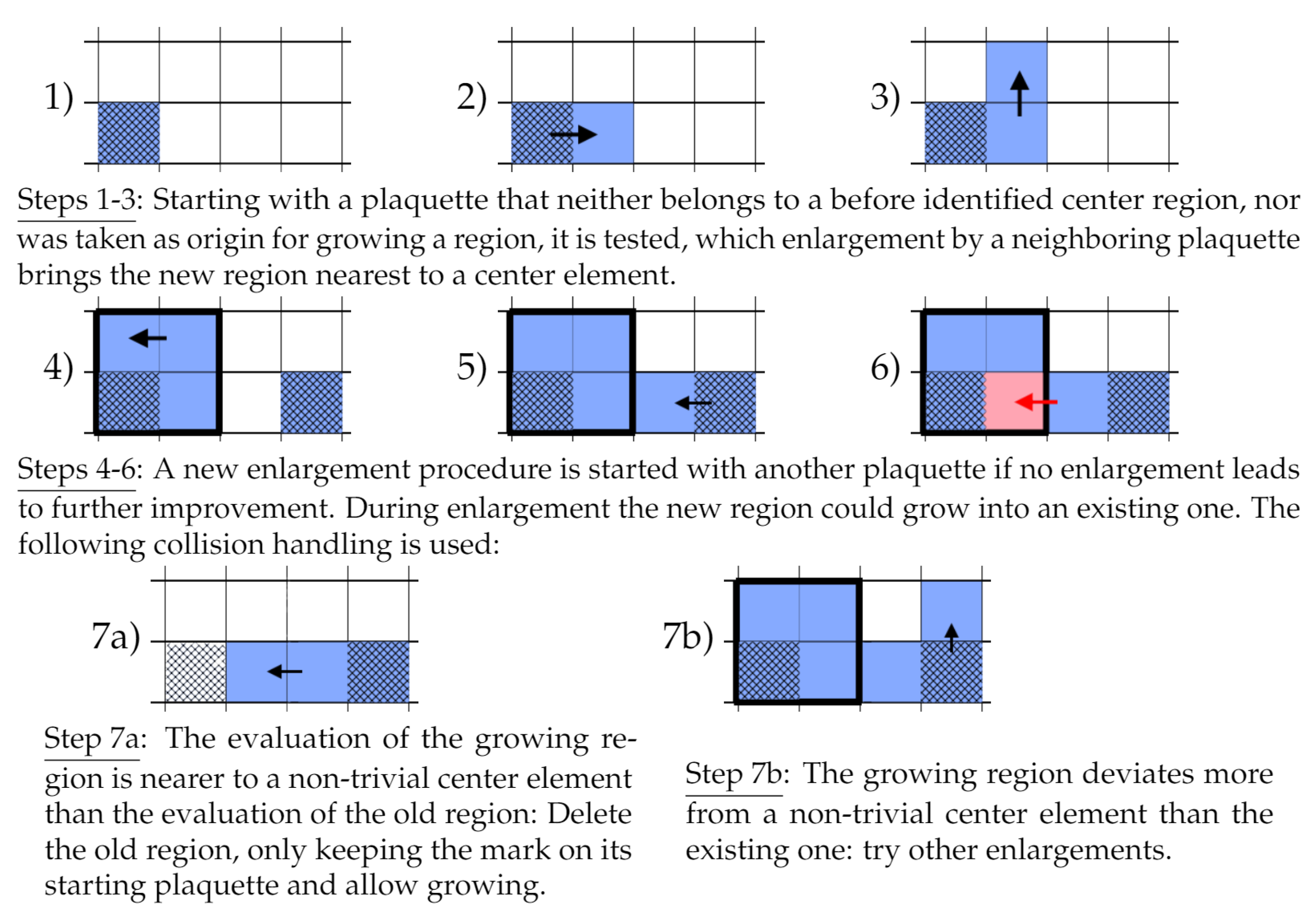
The non-trivial center regions are used to guide this procedure to prevent the problems found by Bornyakov et al. [16]. The detection of such non-trivial center regions is based on enlarging regions until they get as close as possible to non-trivial center elements. This quite calculation-intensive procedure is depicted in Figure 2.

As not all resulting regions are evaluated sufficiently near to a non-trivial center element, we take only those into account which are sufficiently near to non-trivial center elements.

During the gauge-fixing, only such gauge matrices $\Omega$ are allowed that preserve the sign of the non-trivial center regions. As this causes the rejection of some gauge matrices, the number of required simulated annealing steps until convergence of the gauge functional might increase.

After gauge fixing and projection, plaquettes are identified that evaluate non-trivial center elements. These are dubbed P-plaquettes and considered to be pierced by a P-vortex.

If the number of P-plaquettes is smaller than the number of non-trivial center regions used to guide the gauge-fixing procedure, this is a clear indication of a failing vortex detection. For each value of $\beta$, the proportion of configurations where this is the case is determined. This allows to quantify the loss of the vortex-finding property besides quantifying it directly via the string tension of the center-projected configurations.

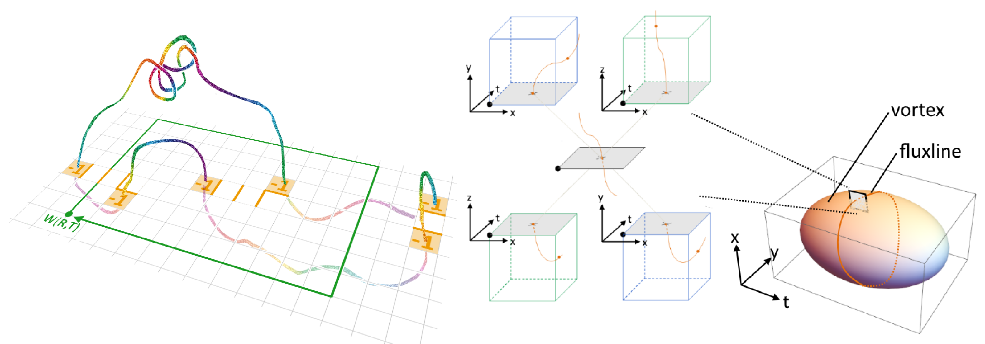
The further analysis is performed in the full SU(2) configurations. For each P-plaquette, a non-trivial center region that encloses the P-plaquette is identified. This center region is considered to be pierced by the thick vortex detected by the P-vortex. Figure 3 depicts the relation between P-vortices, thick vortices and the non-trivial center regions.

The cross-section of the flux building thethick vortex, $A_{\mathrm{vort}}$, is measured by counting the plaquettes that build up the non-trivial center regions enclosing the corresponding thick vortex. In each configuration, we determine minimal, average and maximal cross-sections.

The string tension $\sigma$ is determined via Creutz ratios $\chi$ calculated in the center projected configurations

$$\sigma \approx \chi (R,T)=-ln\frac{\langle W(R+1,T+1)\rangle \langle W(R,T)\rangle }{\langle W(R,T+1)\rangle \langle W(R+1,T)\rangle },$$

(3)

with $R\times T$ Wilson loops $W(R,T)$. As the Coloumb-part of the potential is strongly suppressed after projecting to the center degrees of freedom, the linear part corresponding to a non-vanishing string tension is already reproduced with small loop sizes, as we saw in references [14,15,17]. Symmetric Creutz ratios are used and the average of $\chi (1,1)$ and $\chi (2,2)$ is taken to determine the string tension. Our study is based on the data generated in reference [5], where we did not save a sufficiently wide range of Wilson loop data.

Assuming independence of vortex piercings, the string tension can also be related to the vortex density ${\varrho }_{vort}$, the number of P-plaquettes per unit volume, via

$$\sigma \approx -\ln (1-2\times {\varrho }_{\mathrm{vort}}).$$

(4)

The requirement of uncorrelated piercing is only fulfilled if the vortex surface is strongly smoothed, otherwise this simple equation overestimates the string tension.

The working hypothesis is that the loss of the vortex-finding property, observed via a loss of the string tension, when cooling is applied, can be related to a thickening of the vortices. We will try to model the loss of the vortex density based on an analysis of the geometric structure of center vortices.

3. Results

The different measurements are performed for a lot of different values of $\beta$ and several cooling steps. So as not to overload the visualizations only a part of the intermediate results is depicted, showing only specific numbers of cooling steps and restricting to a smaller interval of $\beta$-values. Those parts of the data that are dominated by finite size effects are identified and excluded from the further analysis.

Starting with the quantification of the vortex-finding property presented in Figure 4, some troubles are brought to light. The proportion of configurations where fewer P-plaquettes have been identified than non-trivial center regions exist, rises rapidly when passing a specific value of $\beta$. This specific value depends on the lattice size and the number of cooling steps.

When reducing the lattice size or increasing the number of cooling steps, the loss of the vortex-finding property occurs at lowered values of $\beta$. The proportion depicted seems to saturate at about 30%, except for 10 cooling steps at a lattice of size $8^4$, where it reaches higher values. The fact that some non-trivial center regions have no corresponding P-plaquettes after gauge fixing and projection to the center degrees of freedom hints at a possible explanation for part of the lost string tension. The gauge functional given in Equation (2) is local in the sense that each gauge matrix $\Omega$ is solely based on the eight gluonic links connected to the specific lattice point. Farther distances than a single lattice spacing are not directly taken into account. In contrast, the detection of the non-trivial center regions is, in a sense, more physical as it is based solely on gauge-independent quantities, that is, the evaluation of arbitrary big Wilson loops. When detecting P-vortices in smooth configurations and high lattice resolutions, the center flux can be distributed over many link variables. Each of these links can evaluate arbitrarily close to the trivial center element, although a Wilson loop build by the links can evaluate arbitrarily near to the non-trivial center element. In such a scenario, a gauge-fixing procedure, only taking the vicinity of lattice points into account, will likely fail and result in an underestimated string tension.

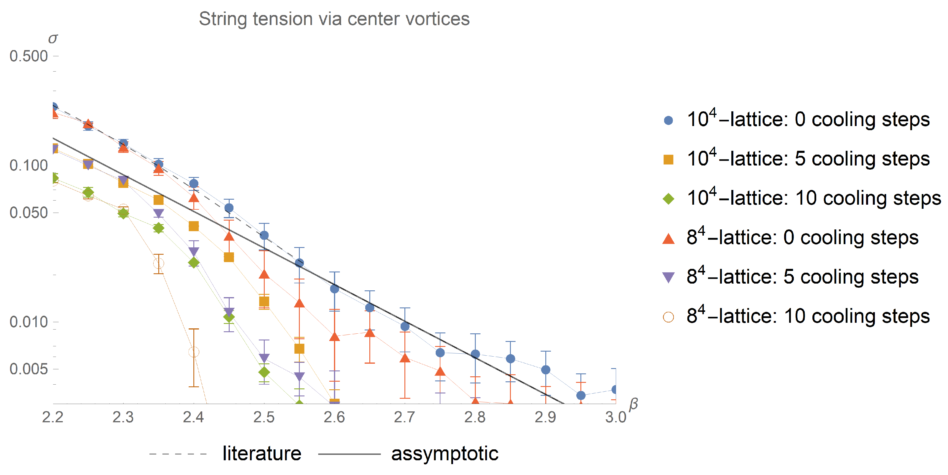
Looking at the Creutz ratios depicted in Figure 5 two possibly intertwined effects can be observed.

At sufficiently low values of $\beta$, the string tension is independent of the lattice size, but decreases with an increasing number of cooling steps. Of interest is that, for sufficiently small values of $\beta$, the deviation from the asymptotic prediction decreases with a rising value of $\beta$—for example, the ${10}^4$-lattice starts at 10 cooling steps with an underestimation of the asymptotic string tension of $50\%\pm 1\%$ at $\beta =2.1$, improving to $40.8\%\pm 0.4\%$ at $\beta =2.25$. At higher values of $\beta$, the independence from the lattice size no longer holds. For different lattice sizes, a sudden decrease in the string tension occurs at different values of $\beta$. The respective $\beta$-values are compatible for different numbers of cooling steps. The dependency on the lattice size and the independence on the number of cooling steps hint at finite size effects, but finite size effects do not give a direct explanation of the reduction in the string tension at lower values of $\beta$: We do not observe a dependency on the lattice size in the low $\beta$-regime. Based on the deviations of the string tensions for different lattice sizes, we expect finite size effects to occur at length scales around $1.3$ fm, independent of cooling: observing that the lattice of size $8^4$ deviates from the ${10}^4$-lattice at $\beta \approx 2.3$, corresponding to a lattice spacing of $a\approx 0.165$, we acquire a physical lattice extend around $1.32$ fm for the smaller lattice. The finite size effects on the bigger lattice set in at $\beta$ between approximately $2.35$ and $2.4$, resulting in a length scale between approximately $1.2$ fm and $1.4$ fm. This length scales are compatible with the findings of Kovacs and Tomboulis [18]. In Ref. [5] we also found color-homogeneous regions embedded in the vortex surface with roughly the same diameters. Similar distances can also be found between neighbouring piercings of a Wilson loop, extracted from the vortex density, as will be seen in Table 4.

A relation to the thickness $A_{\mathrm{vort}}$ of center vortices is suspected and points towards possible further analysis. The possibility of a thick vortex expanding due to a spreading of the center flux was already suggested by Kovacs and Tomboulis in [19]. Assuming a circular cross-section of the flux tube, its diameter can be calculated as

$$d_{\mathrm{flux}}=2\times \underset{r_{\mathrm{flux}}}{\underbrace{\sqrt{\frac{A_{\mathrm{vort}}}{\pi }}}},$$

(5)

with $A_{\mathrm{vort}}$ being the area of the flux cross-section. That flux lines are closed requires that within each two-dimensional slice through the lattice at least two vortex piercings can find place. This give a criteria on the lattice extent L

$$L>2\ast d_{\mathrm{flux}}.$$

(6)

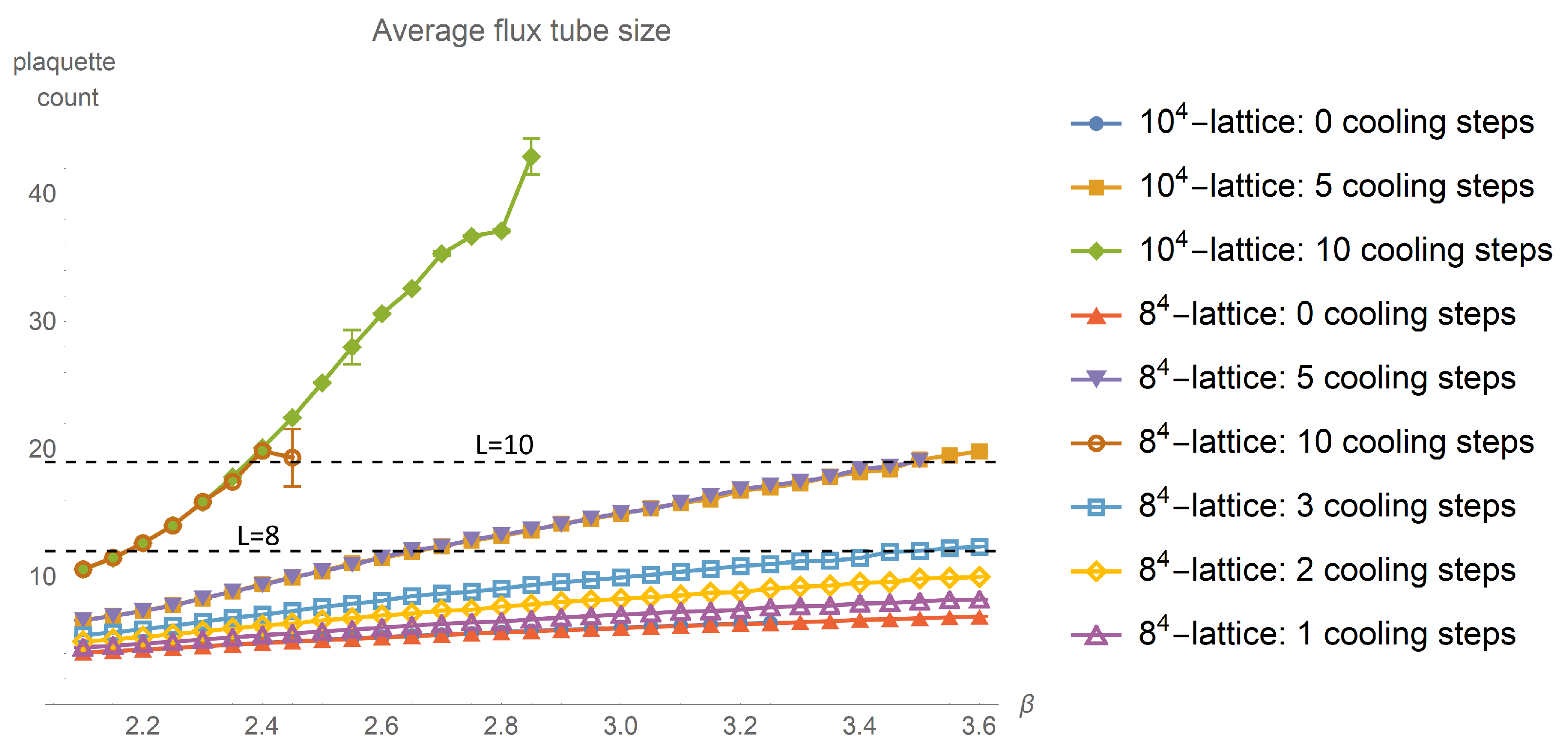
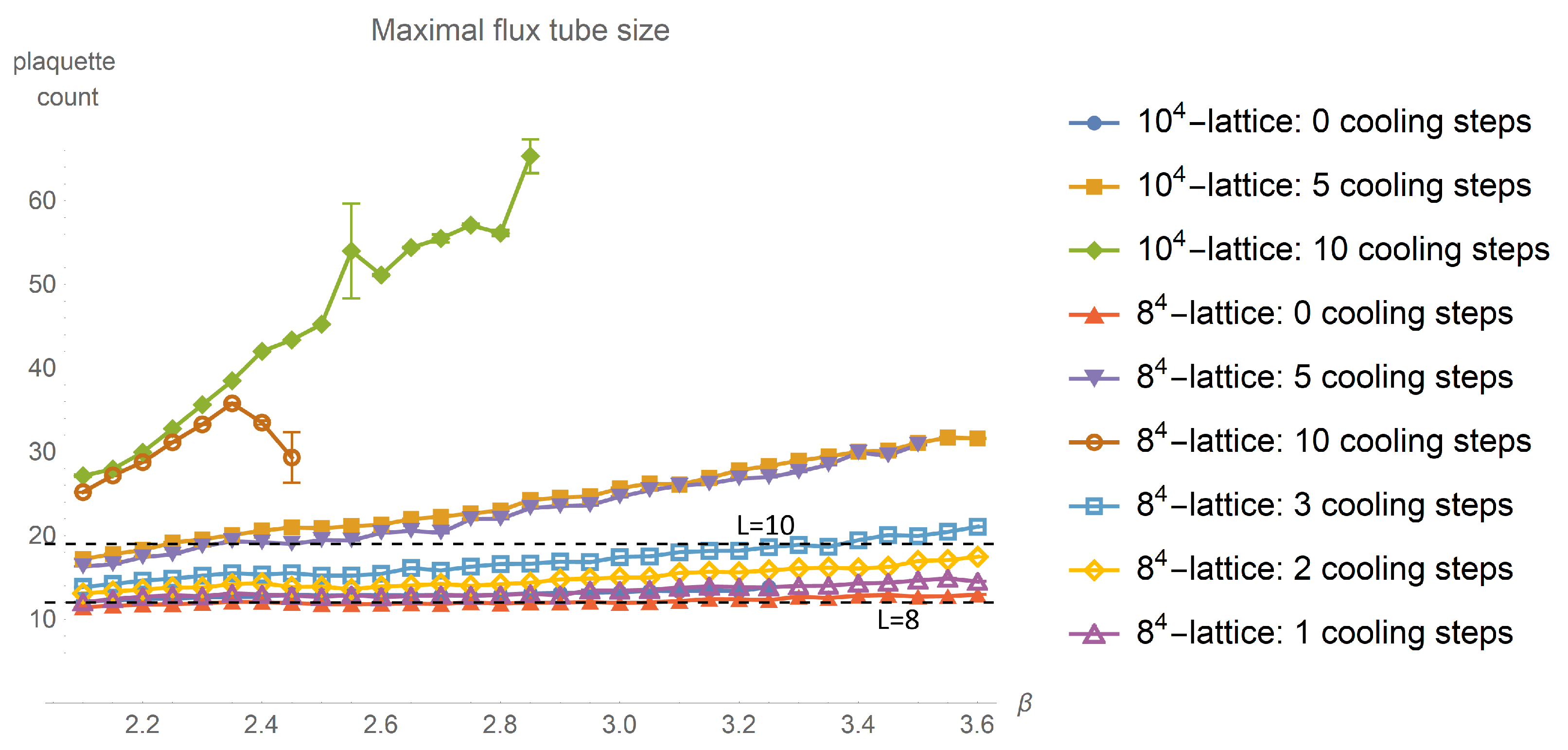
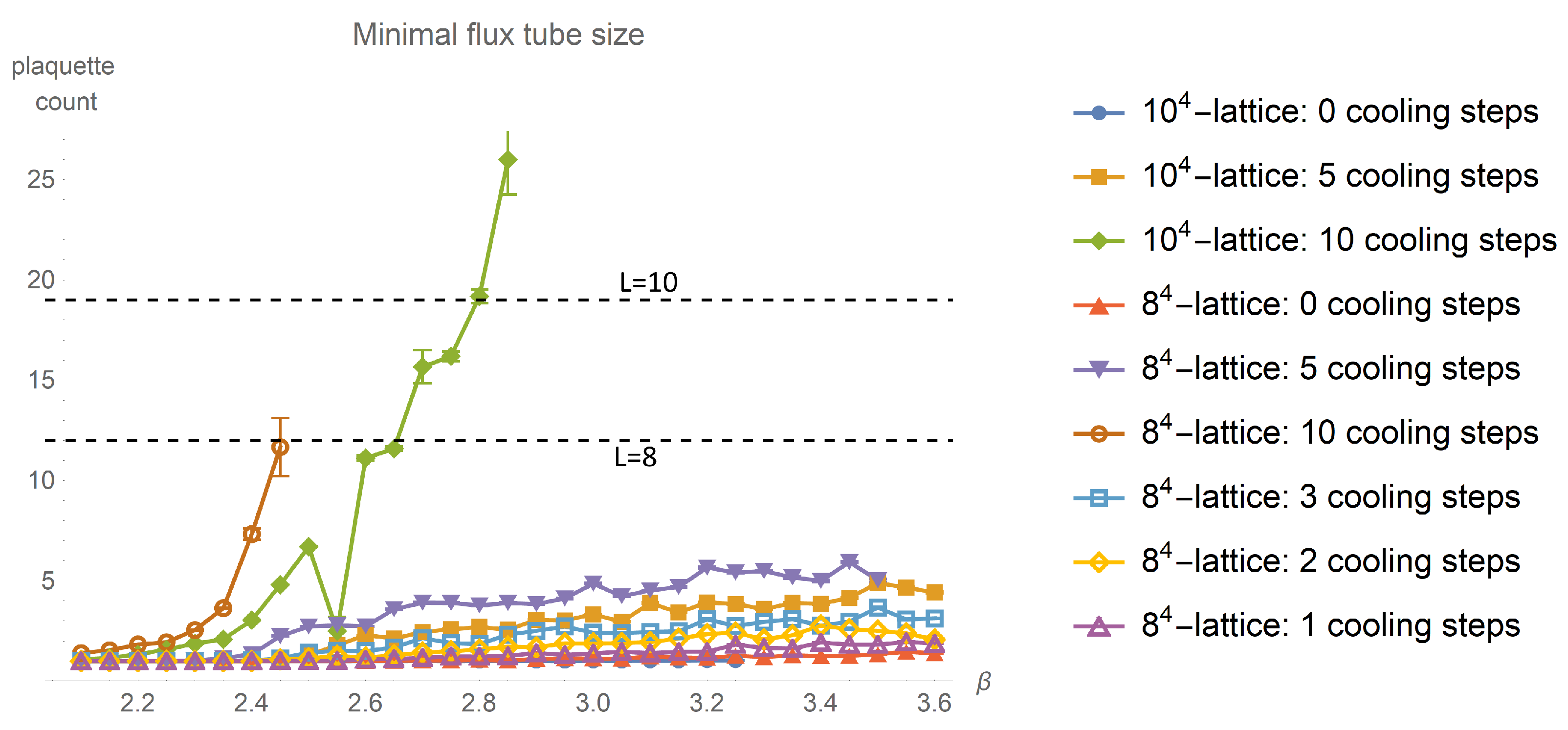
If $A_{\mathrm{vort}}$ measured by a plaquette count exceeds 19 for a lattice of size ${10}^4$, or 12 for a lattice of size $8^4$, we can expect finite size effects to step in. These thresholds are of relevance for the average, minimal and maximal flux tube cross-section depicted in Figure 6, Figure 7 and Figure 8. The mean flux tube cross-section presented in Figure 6 shows that we have to restrict to relative low values of $\beta$ to stay away from finite size effects.

Taking a look at the maximal flux tube cross-section depicted in Figure 7, we can expect finite size effects at even lower values of $\beta$: None of the data with 10 cooling steps can be expected to be free of finite size effects.

The lattice of size $8^4$ could be too small even without any cooling applied. With cooling and increasing $\beta$ the different lattice sizes become more and more incompatible. This may be caused by finite size effects and insufficient statistics. Still, the overall behaviour with cooling is qualitatively reproduced and allows the gain of another estimate on the growth rate.

Looking at the minimal tube size depicted in Figure 8 an even more sudden rise in the cross-section can be observed.

We expect that the minimal flux tube cross-sections starts to grow with a certain $\beta$, where the high action density of non-trivial plaquettes leads to a suppression within the path integral. This causes a dependency on the lattice size due to the reduced statistics. For sufficiently low values of $\beta$ and sufficiently low numbers of cooling steps, the minimal flux tube cross-section is given by exactly one plaquette, independent of $\beta$ and the number of cooling steps. We restrict further analysis to ${10}^4$-lattices with $\beta \le 2.3$ and, at most, five cooling steps. Nevertheless, we depict the full data in all relevant figures to allow for a check of the plausibility of our model by looking at the specific deviations of the data from our prediction.

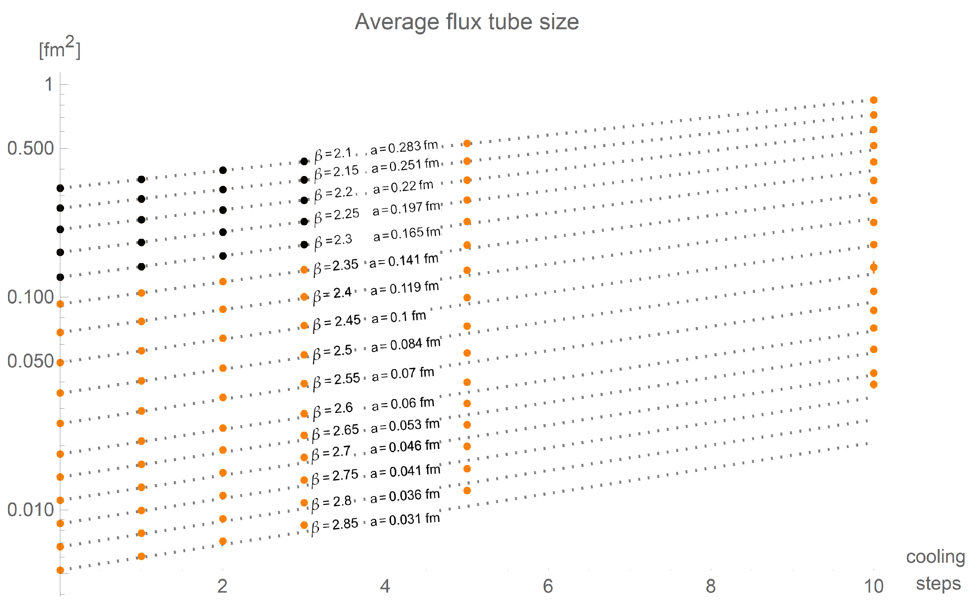
Assuming an exponential growth in the flux tubes’ cross-section with an increase in the number of cooling steps, a model of the form

$$A_{\mathrm{vort}}\left(N_{\mathrm{cool}}\right)=A_{\mathrm{vort}}\left(0\right)e^{N_{\mathrm{cool}}(g_{\mathrm{cool}}+g_{\mathrm{discret}}a)}$$

(7)

is fit to the data, with $N_{\mathrm{cool}}$ being the number of cooling steps and a the lattice spacing. The fit-parameter $g_{\mathrm{cool}}$ corresponds to the exponential growth in the flux tube with cooling. As the tube size is measured by counting plaquettes, we have to account for discretization effects. This is done by adding another fit-parameter $g_{\mathrm{discret}}$ in the exponent, related to the lattice spacing and the number of cooling steps. The two parameters are not necessarily constant as they can depend on the specific structure of interest. We restrain from carrying along another index: In the following, the values of these two parameters are to be considered only with respect to the specific context. They differ for the average cross-sections and the maximal cross-sections of flux tubes. The fit of this model to the average flux tube sizes is shown in Figure 9 in physical units. The fit is done for small $\beta$ and cooling steps indicated by black points.

The fit, dashed lines reproduce the data well until the expected onset of finite size effects for cross-sections, increasing with the number of cooling steps and $\beta$. This onset is compatible to the estimates in Equation (6) and will be discussed later. At present, we concentrate on the growth in the flux tube cross-section described by the fit parameters given in

Table 2. The parameters of the model described by Equation (7) and depicted in Figure 9 for average cross-sections are shown.

Average Cross-Sections	Estimate	t-Statistic	p-Value
$g_{\mathrm{cool}}$	0.14(1)	13.6393	$6.3\times {10}^{-11}$
$g_{\mathrm{discret}}$	−0.17(5) fm−1	−3.62376	$1.9\times {10}^{-3}$

. The suspected exponential growth of $A_{\mathrm{vort}}$ is confirmed by the good quality of the fit for positive $g_{\mathrm{cool}}$, even for larger values of $\beta$ and cooling steps.

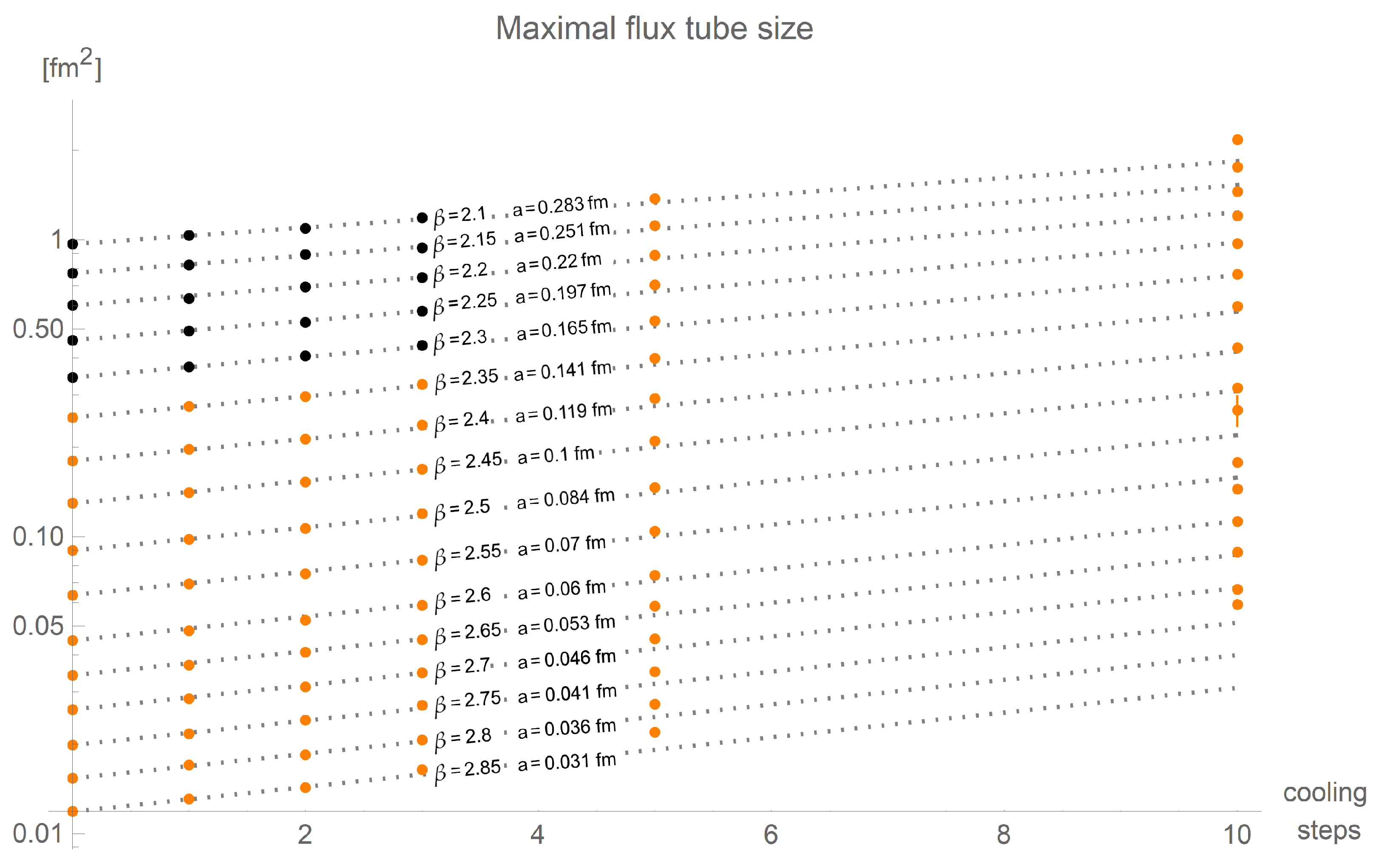
The negative value of $g_{\mathrm{discret}}$ reflects the decreasing slope of the dashed lines with increasing $\beta$, indicating an influence of the lattice resolution: a coarser lattice reduces the growth of $A_{\mathrm{vort}}$. The overall behaviour of $A_{\mathrm{vort}}$ is qualitatively reproduced by the maximal cross-sections, as depicted in Figure 10.

Only the growth has slowed down, as can be seen in the values given in

Table 3. The parameters of the model described by Equation (7) and depicted in Figure 10 for maximal cross-sections are shown.

Maximal Cross-Sections	Estimate	t-Statistic	p-Value
$g_{\mathrm{cool}}$	0.0999(10)	9.1369	$3.5\times {10}^{-8}$
$g_{\mathrm{discret}}$	−0.13(5) fm−1	−2.61939	$1.7\times {10}^{-2}$

.

This implies that the growthin $A_{\mathrm{vort}}$ with increased cooling is limited.

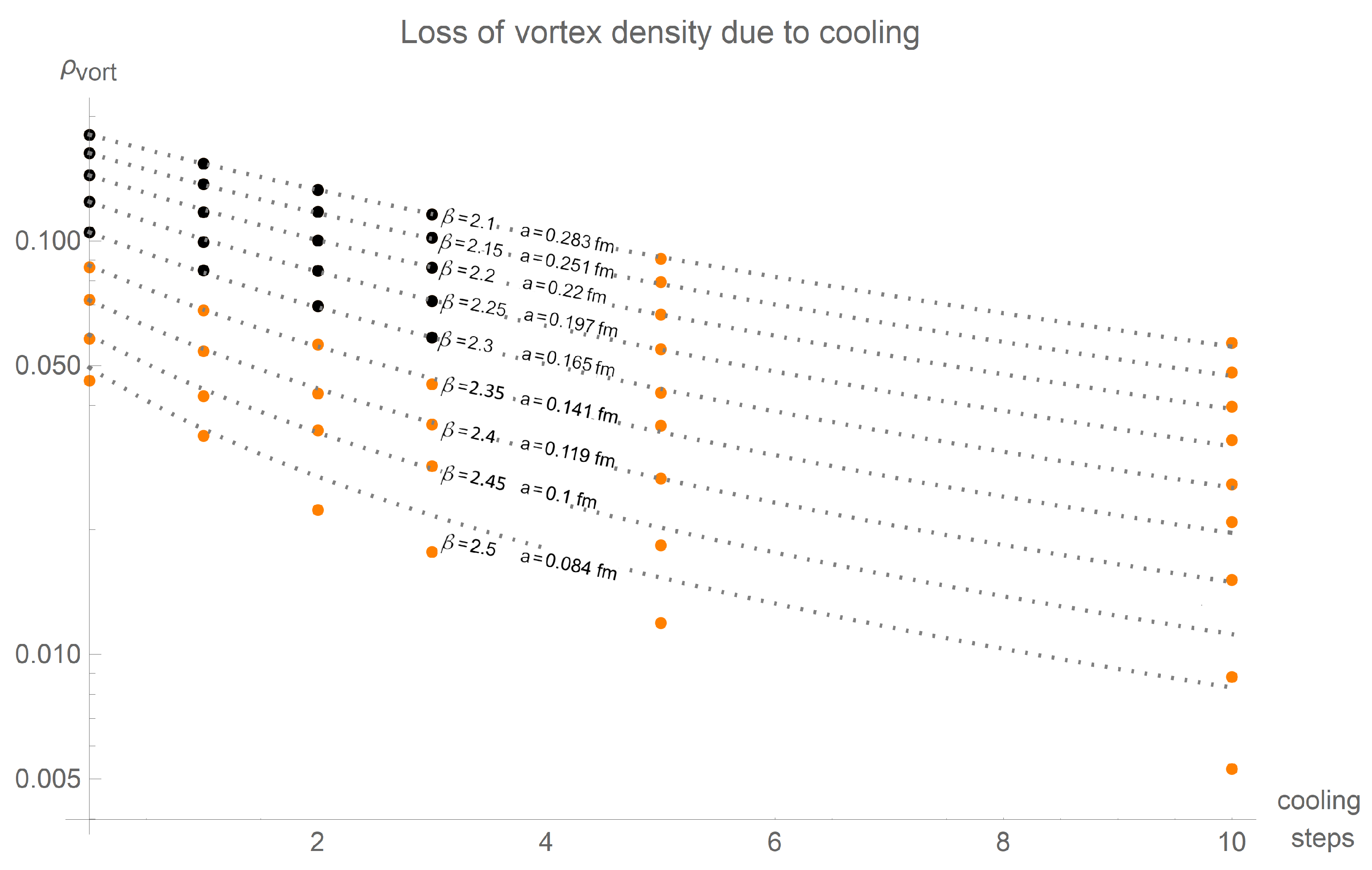
A further influence of cooling is a smoothing of the vortex surface. We will now model this smoothing and show that the vortex flux tubes can be thickened without pushing each other apart. The vortex density ${\varrho }_{\mathrm{vort}}$ allows to gain information about the distance of the vortex centers. Here, we have to take into account that some of the P-plaquettes belong to correlated piercings and can be attributed to short-range fluctuations. We define the quantity $A_{\max }$ as the non-overlapping area around vortex centers.

The vortex density ${\varrho }_{\mathrm{vort}}$ is usually calculated by dividing the number P-plaquettes by the total plaquette number. Given enough statistics, it can be determined by counting the number of piercings $N_{\mathrm{vort}}$ within a sufficiently large Wilson loop of Area $A_{\mathrm{loop}}$ build by $N_{\mathrm{loop}}$ plaquettes

$$\begin{array}{c}\hfill {\varrho }_{\mathrm{vort}}=\frac{N_{\mathrm{vort}}}{N_{\mathrm{loop}}}=\frac{N_{\mathrm{vort}}}{A_{\mathrm{loop}}\ast a^{-2}}=\frac{N_{\mathrm{vort}}}{(A_{\mathrm{free}}+N_{\mathrm{vort}}\ast A_{\max })\ast a^{-2}}.\end{array}$$

(8)

In the last identity, we have split the area of the loop into two non-overlapping parts: each piercing is enclosed by circular area given by $A_{\max }$ and $A_{\mathrm{free}}$ covers the remaining part of the loop. When cooling is applied, we have to take into account that $A_{\max }$ grows.

$${\varrho }_{\mathrm{vort}}\left(N_{\mathrm{cool}}\right)=\frac{N_{\mathrm{vort}}}{(A_{\mathrm{free}}+N_{\mathrm{vort}}\ast (A_{\max }\left(0\right)+\delta A_{\max }\left(N_{\mathrm{cool}}\right)))\ast a^{-2}}.$$

(9)

Using $A_{\mathrm{loop}}=A_{\mathrm{free}}+N_{\mathrm{vort}}\ast A_{\max }\left(0\right)$ and a model of the form given in Equation (7) for $A_{\max }\left(N_{\mathrm{cool}}\right)$ we attain $\delta A_{\max }=A_{\max }\left(0\right)(e^{N_{\mathrm{cool}}(g_{\mathrm{cool}}+g_{\mathrm{discrete}}a)}-1)$. It follows

$${\varrho }_{\mathrm{vort}}\left(N_{\mathrm{cool}}\right)=\frac{{\varrho }_{\mathrm{vort}}\left(0\right)}{1+{\varrho }_{\mathrm{vort}}\left(0\right)A_{\max }\left(0\right)a^{-2}(e^{N_{\mathrm{cool}}(g_{\mathrm{cool}}+g_{\mathrm{discrete}}a)}-1)}.$$

(10)

We fit $g_{\mathrm{cool}}$, $g_{\mathrm{discrete}}$ and $A_{\max }\left(0\right)$ to the measurements of ${\varrho }_{\mathrm{vort}}$. The measured data and the fit are shown in Figure 11.

The respective fit parameters are listed in

Table 4. The parameters of the model described by Equation (10) for the loss of the vortex density during cooling.

Vortex Density	Estimate	t-Statistic	p-Value
$g_{\mathrm{cool}}$	0.035(1)	26.5368	$2.8\times {10}^{-15}$
$g_{\mathrm{discret}}$	0.066(2) fm−1	27.6254 fm−1	$1.5\times {10}^{-15}$
$A_{\max }\left(0\right)$	1.41(5) fm2	25.8937 fm2	$4.2\times {10}^{-15}$

.

The value of $A_{\max }\left(0\right)$ is larger than the flux tube cross-sections depicted in Figure 9. This, and the fact that the value of $g_{\mathrm{cool}}$, for the vortex density is smaller than those of the vortex flux tube cross-sections indicate that the majority of piercings remain separated from one another even when cooling is applied. Assuming circular geometry, we can calculate the minimal possible distance between vortex centers

$$d_{\mathrm{center}}\left(N_{\mathrm{cool}}\right)=2\sqrt{\frac{A_{\max }\left(N_{\mathrm{cool}}\right)}{\pi }}.$$

(11)

To determine how many cooling steps are possible, we need to know how much the vortices can grow by cooling without getting into conflict. We estimate the minimal available separation by

$$s_{\mathrm{flux}}\left(N_{\mathrm{cool}}\right)=\underset{d_{\mathrm{center}}\left(0\right)}{\underbrace{2\sqrt{\frac{A_{\max }\left(0\right)}{\pi }}}}-\underset{d_{\mathrm{flux}}\left(N_{\mathrm{cool}}\right)}{\underbrace{2\sqrt{\frac{A_{\mathrm{vort}}\left(N_{\mathrm{cool}}\right)}{\pi }}}}.$$

(12)

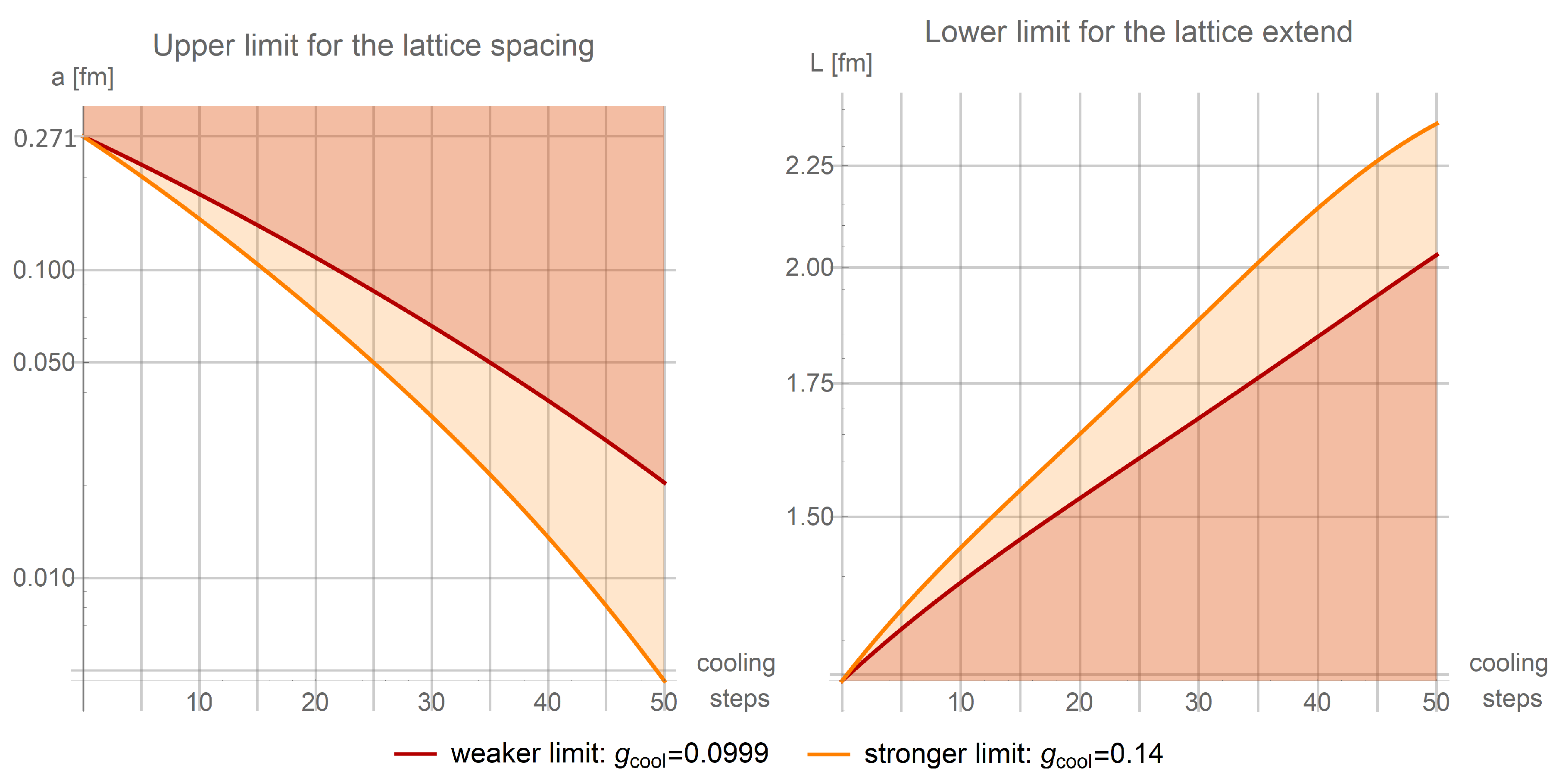
We use $d_{\mathrm{center}}\left(0\right)$, the average distance between piercings when no loss of the vortex density occurred, and subtract the average diameter of the flux tubes $d_{\mathrm{flux}}\left(N_{\mathrm{cool}}\right)$ with cooling applied. If $s_{\mathrm{flux}}\left(N_{\mathrm{cool}}\right)$ becomes smaller than one lattice spacing, our methods of center vortex detection are likely to fail: we can no longer find two non-overlapping non-trivial center regions enclosing the thick vortex flux tubes. This allows for a limit for the lattice spacing to be derived, a, given in Equation (13) together with a limit on L based on Equation (6)

$$a<s_{\mathrm{flux}}\mathrm{and}L>\mathrm{Max}(2\overline{d_{\mathrm{flux}}},\mathrm{Max}\left(d_{\mathrm{flux}}\right)).$$

(13)

The requirement for the lattice extent L is based on the fact that two vortex piercings have to fit in every two-dimensional slicing through the lattice. Assuming a vanishing minimal flux tube size, the limit is given either by two times the average diameter $\overline{d_{\mathrm{flux}}}$ or one times the maximal diameter $\mathrm{Max}\left(d_{\mathrm{flux}}\right)$—whatever is bigger. The assumption of a vanishing minimal flux tube size is an approximation: on the lattice, the minimal size is given by exactly one plaquette, which is normally negligible in comparison to the lattice extent.

Using what we learned so far, we can evaluate these inequalities and find numerical values for the upper limit of a and the lower limit of L. These are depicted in Figure 12 and will now be discussed. Discretization effects are neglected by setting $g_{\mathrm{discret}}=0$. Fitting the average flux tube cross-sections for configurations without cooling for $2.1\le \beta \le 2.3$, see Figure 9, by a polynom up to quadratic order with respect to the lattice spacing a gives

$$\overline{A_{\mathrm{vort}}}\left(0\right)\approx 3.367\left(38\right)a^2+0.200\left(9\right)\mathrm{fm}a,$$

(14)

compatible with the values we found in [20]. A fit to the maximal cross-sections without cooling for $2.1\le \beta \le 2.3$, see Figure 10, results in higher fit parameters

$$Max\left(A_{\mathrm{vort}}\left(0\right)\right)\approx 11.3\left(2\right)a^2+0.224\left(37\right)\mathrm{fm}a.$$

(15)

Using this fit and Equation (12) with $A_{\max }\left(0\right)$ from Table 4 we obtain an upper limit for the lattice spacing that depends on the number of cooling steps and $g_{\mathrm{cool}}$. With this limit, we can determine a lower limit for the required lattice extent. Both limits are shown in Figure 12 for the two different values of $g_{\mathrm{cool}}$ resulting from average and maximal flux tube sizes from Table 2 and Table 3. Let us remember how these limits were derived. Closed flux lines require sufficient room for two piercings within each two dimensional slice through the lattice—a lower limit for the lattice extent arises.

Taking the stronger limits with $g_{\mathrm{cool}}=0.14$, we determine the corresponding limits of $\beta$ for given lattice size and number of cooling steps. In

Table 5. For different numbers of cooling steps and different lattice extents, the table gives a lower and an upper limit for $\beta$. “None” indicates that the limits exclude one another.

${\mathit{N}}_{\mathbf{cool}}\setminus \mathit{L}$	8	10	14	20	30	40	50
0	$\begin{array}{c}2.12\\ 2.32\end{array}$	$\begin{array}{c}2.12\\ 2.39\end{array}$	$\begin{array}{c}2.12\\ 2.48\end{array}$	$\begin{array}{c}2.12\\ 2.58\end{array}$	$\begin{array}{c}2.12\\ 2.73\end{array}$	$\begin{array}{c}2.12\\ 2.84\end{array}$	$\begin{array}{c}2.12\\ 2.92\end{array}$
1	$\begin{array}{c}2.14\\ 2.31\end{array}$	$\begin{array}{c}2.14\\ 2.38\end{array}$	$\begin{array}{c}2.14\\ 2.48\end{array}$	$\begin{array}{c}2.14\\ 2.58\end{array}$	$\begin{array}{c}2.14\\ 2.73\end{array}$	$\begin{array}{c}2.14\\ 2.83\end{array}$	$\begin{array}{c}2.14\\ 2.91\end{array}$
2	$\begin{array}{c}2.16\\ 2.31\end{array}$	$\begin{array}{c}2.16\\ 2.38\end{array}$	$\begin{array}{c}2.16\\ 2.47\end{array}$	$\begin{array}{c}2.16\\ 2.58\end{array}$	$\begin{array}{c}2.16\\ 2.72\end{array}$	$\begin{array}{c}2.16\\ 2.83\end{array}$	$\begin{array}{c}2.16\\ 2.91\end{array}$
3	$\begin{array}{c}2.19\\ 2.3\end{array}$	$\begin{array}{c}2.19\\ 2.37\end{array}$	$\begin{array}{c}2.19\\ 2.47\end{array}$	$\begin{array}{c}2.19\\ 2.57\end{array}$	$\begin{array}{c}2.19\\ 2.71\end{array}$	$\begin{array}{c}2.19\\ 2.82\end{array}$	$\begin{array}{c}2.19\\ 2.9\end{array}$
5	$\begin{array}{c}2.23\\ 2.29\end{array}$	$\begin{array}{c}2.23\\ 2.36\end{array}$	$\begin{array}{c}2.23\\ 2.46\end{array}$	$\begin{array}{c}2.23\\ 2.56\end{array}$	$\begin{array}{c}2.23\\ 2.7\end{array}$	$\begin{array}{c}2.23\\ 2.81\end{array}$	$\begin{array}{c}2.23\\ 2.89\end{array}$
10	None	$\begin{array}{c}2.34\\ 2.34\end{array}$	$\begin{array}{c}2.34\\ 2.44\end{array}$	$\begin{array}{c}2.34\\ 2.54\end{array}$	$\begin{array}{c}2.34\\ 2.67\end{array}$	$\begin{array}{c}2.34\\ 2.78\end{array}$	$\begin{array}{c}2.34\\ 2.86\end{array}$
15	None	None	None	$\begin{array}{c}2.44\\ 2.52\end{array}$	$\begin{array}{c}2.44\\ 2.65\end{array}$	$\begin{array}{c}2.44\\ 2.76\end{array}$	$\begin{array}{c}2.44\\ 2.84\end{array}$
20	None	None	None	None	$\begin{array}{c}2.54\\ 2.63\end{array}$	$\begin{array}{c}2.54\\ 2.73\end{array}$	$\begin{array}{c}2.54\\ 2.82\end{array}$
25	None	None	None	None	None	$\begin{array}{c}2.66\\ 2.71\end{array}$	$\begin{array}{c}2.66\\ 2.79\end{array}$

some numerical values are shown.

We now look at the meaning of these limits for the string tension. In Figure 5, we observe that the deviation from the asymptotic prediction decreases with increasing $\beta$ in the low $\beta$-regime. We believe that this behaviour holds within the $\beta$-intervals of Table 5. The upper limit of $\beta$ can be extended by increasing the lattice size. It would be interesting to see if this alone suffices to restore full compatibility with the asymptotic string tension with modest cooling, but the required computational power might exceed our present capabilities.

4. Discussion

Using non-trivial center regions we analyzed how Pisa-cooling influences the cross-sections of thick center vortices. We found an exponential growth that slows down with increasing cross-sections. By geometric arguments, we derived an upper limit for the lattice spacing above which discretization effects trouble the vortex detection and a lower limit for the lattice extent where finite size effects set in. This window gets smaller with cooling and decreasing lattice extent. Cooling results in deviations from the asymptotic behaviour: an underestimation of the string tension occurs. Within the window, increasing $\beta$ leads to better agreement with the asymptotic behaviour. It would be interesting to see whether the string tension calculated on the projected lattice is, in fact, fully restored with sufficiently large $\beta$ or if only a partial restoration occurs.

By improving the method of center vortex detection, it might be possible to soften the aforementioned limits. The method of vortex detection used in this work was based on the direct maximal center gauge guided by non-trivial center regions [13,14,15]: we identify regions whose perimeter evaluates to the non-trivial center element and preserve their evaluation during gauge-fixing and center projection. This approach comes with three possibilities of improvement.

The growth in the flux tube due to cooling results in the non-trivial center factors within the evaluation of Wilson loops being spread over more and more links. In the original direct maximal center gauge the contribution to the gauge functional at a given site x is determined by its attached links only. By taking farther links into account, the troubles arising from the spread of the center flux may be counteracted.

When two thick vortices are not separated by at least one lattice spacing, the identification of non-trivial center regions enclosing the single piercings might fail. The original method used for the detection of non-trivial center regions is based on enlarging the perimeter of Wilson loops while preventing overlaps of the resulting regions: if overlaps occurred, the region that evaluates to a higher trace is deleted. By allowing overlaps, an improvement might be possible: more non-trivial center regions are kept to guide the further gauge-fixing procedure.

With rising number of cooling steps, more non-trivial center regions than P-plaquettes were found: The direct maximal center gauge failed to preserve some of the non-trivial center regions. This could be counteracted by inserting non-trivial factors before starting the simulated annealing procedure used to maximize the gauge functional. These non-trivial factors should guarantee that each non-trivial center region evaluates to the non-trivial center element when evaluated in the center projected configuration.

References

1. Del Debbio, L.; Faber, M.; Giedt, J.; Greensite, J.; Olejnik, S. Detection of center vortices in the lattice Yang-Mills vacuum. Phys. Rev. 1998, D58, 094501. [Google Scholar] [CrossRef] [Green Version]
2. Faber, M.; Höllwieser, R. Chiral symmetry breaking on the lattice. Prog. Part. Nucl. Phys. 2017, 97, 312–355. [Google Scholar] [CrossRef] [Green Version]
3. Höllwieser, R.; Schweigler, T.; Faber, M.; Heller, U.M. Center Vortices and Chiral Symmetry Breaking in SU(2) Lattice Gauge Theory. Phys. Rev. 2013, D88, 114505. [Google Scholar] [CrossRef] [Green Version]
4. Höllwieser, R.; Schweigler, T.; Faber, M.; Heller, U.M. Center vortices and topological charge. In Proceedings of the Xth Quark Confinement and the Hadron Spectrum—PoS(Confinement X), Munich, Germany, 21 May 2013. [Google Scholar] [CrossRef] [Green Version]
5. Golubich, R.; Golubich, R.; Faber, M. Properties of SU(2) Center Vortex Structure in Smooth Configurations. Particles 2021, 4, 93–105. [Google Scholar] [CrossRef]
6. Kovacs, T.G.; Tomboulis, E.T. On P vortices and the Gribov problem. Phys. Lett. B 1999, 463, 104–108. [Google Scholar] [CrossRef] [Green Version]
7. Bali, G.S.; Schlichter, C.; Schilling, K. Observing long color flux tubes in SU(2) lattice gauge theory. Phys. Rev. D 1995, 51, 5165–5198. [Google Scholar] [CrossRef] [PubMed] [Green Version]
8. Booth, S.P.; Hulsebos, A.; Irving, A.C.; McKerrell, A.; Michael, C.; Spencer, P.S.; Stephenson, P.W. SU(2) potentials from large lattices. Nucl. Phys. 1993, B394, 509–526. [Google Scholar] [CrossRef] [Green Version]
9. Michael, C.; Teper, M. Towards the Continuum Limit of SU(2) Lattice Gauge Theory. Phys. Lett. 1987, B199, 95–100. [Google Scholar] [CrossRef]
10. Perantonis, S.; Huntley, A.; Michael, C. Static Potentials From Pure SU(2) Lattice Gauge Theory. Nucl. Phys. 1989, B326, 544–556. [Google Scholar] [CrossRef]
11. Bali, G.S.; Fingberg, J.; Heller, U.M.; Karsch, F.; Schilling, K. The Spatial string tension in the deconfined phase of the (3+1)-dimensional SU(2) gauge theory. Phys. Rev. Lett. 1993, 71, 3059–3062. [Google Scholar] [CrossRef] [PubMed] [Green Version]
12. Campostrini, M.; Di Giacomo, A.; Maggiore, M.; Panagopoulos, H.; Vicari, E. Cooling and the String Tension in Lattice Gauge Theories. Phys. Lett. B 1989, 225, 403–406. [Google Scholar] [CrossRef]
13. Golubich, R.; Faber, M. The Road to Solving the Gribov Problem of the Center Vortex Model in Quantum Chromodynamics. Acta Phys. Pol. B Proc. Suppl. 2020, 13, 59–65. [Google Scholar] [CrossRef]
14. Golubich, R.; Faber, M. Center Regions as a Solution to the Gribov Problem of the Center Vortex Model. Acta Phys. Pol. B Proc. Suppl. 2021, 14, 87. [Google Scholar] [CrossRef]
15. Golubich, R.; Faber, M. Improving Center Vortex Detection by Usage of Center Regions as Guidance for the Direct Maximal Center Gauge. Particles 2019, 2, 491–498. [Google Scholar] [CrossRef] [Green Version]
16. Bornyakov, V.G.; Komarov, D.A.; Polikarpov, M.I.; Veselov, A.I. P vortices, nexuses and effects of Gribov copies in the center gauges. Quantum chromodynamics and color confinement. In Proceedings of the International Symposium, Confinement 2000, Osaka, Japan, 7–10 March 2000; pp. 133–140. [Google Scholar]
17. Dehghan, Z.; Deldar, S.; Faber, M.; Golubich, R.; Höllwieser, R. Influence of Fermions on Vortices in SU(2)-QCD. Preprints 2021, 2021040233. [Google Scholar] [CrossRef]
18. Kovacs, T.G.; Tomboulis, E.T. Vortex structure of the vacuum and confinement. Nucl. Phys. B Proc. Suppl. 2001, 94, 518–521. [Google Scholar] [CrossRef] [Green Version]
19. Kovács, T.G.; Tomboulis, E. Bound on the string tension by the excitation probability for a vortex. Nuclear Phys. B Proc. Suppl. 2000, 83–84, 553–555. [Google Scholar] [CrossRef]
20. Golubich, R.; Faber, M. Thickness and Color Structure of Center Vortices in Gluonic SU(2) QCD. Particles 2020, 3, 444–455. [Google Scholar] [CrossRef]
Figure 1. The geometric relation between piercings, the flux line and the vortex surface is schematically shown. Left: A flux line can be traced by following non-trivial plaquettes (depicted in orange with a “−1”) after transformation to maximal center gauge and projection to the center degrees of freedom. Middle: Each non-trivial plaquette belongs to four elementary cubes, where the flux enters and has to leave through another plaquette. The depicted grey rectangles correspond to the same plaquette. For each cube, the three involved coordinates are indicated. Right: Due to the evolution in time, the flux line (depicted as orange line) forms a closed two-dimensional surface in four-dimensional spacetime.
Universe 07 00122 g001
Figure 2. The non-trivial center regions, used for the gauge-fixing procedure, are detected by repeating the depicted procedure until every plaquette either belongs to an identified region or has already been used as the seed to grow a region. The direction of enlargement of the respective regions is marked by an arrow. Plaquettes that belong to a region are colored; plaquettes already used as seed are shaded. In the final determination of the non-trivial center regions enclosing a thick vortex, no collision handling is performed.
Universe 07 00122 g002
Figure 3. Two-dimensional slices through a four-dimensional lattice are depicted. The vortex detection starts as a best-fit procedure of P-Vortices to thick vortices, indicated by the first arrow. Then, starting from the detected P-plaquettes, non-trivial center regions are identified to reconstruct the thick vortex. These non-trivial center regions are, in general, not rectangular.
Universe 07 00122 g003
Figure 4. The proportion of configurations is depicted where less non-trivial plaquettes have been identified than non-trivial regions exist. The datapoints are joined to guide the eye. Due to the logarithmic scaling of axes, only non-vanishing values are depicted: all lines start with 0% at lower values of β . The interruption of the green line corresponding to the lattice of size 10 4 at 10 cooling steps at β = 2.55 results from a vanishing percentage at the respective β -value. Observe that the curves rise at different values of β for different number of cooling steps and different lattice sizes.
Universe 07 00122 g004
Figure 5. The string tension σ is estimated via an average of the Creutz ratios χ ( 1 , 1 ) and χ ( 2 , 2 ) calculated in center-projected configurations for different numbers of cooling steps and lattice sizes. The datapoints are joined by lines to guide the eye. The literature values correspond to those listed in Table 1; the asymptotic line is given by Equation (1). Observe that, in the low β -regime, an underestimation of the string tension correlates to the number of cooling steps. This underestimation is independent of the lattice size. At higher values of β , finite size effects set in.
Universe 07 00122 g005
Figure 6. The average cross-sections of the flux tubes, measured by counting plaquettes, increases when cooling is applied. It reaches a threshold at which finite size effects are expected to become problematic, shown as a dashed line for the two lattice sizes. Measurements performed on lattices of different size have good compatibility.
Universe 07 00122 g006
Figure 7. The maximal cross-sections of the flux tubes hint at finite size effects. Within our β -interval, only the lattice of size 10 4 stays below the threshold when cooling is applied. With cooling, the different lattice sizes become more and more incompatible.
Universe 07 00122 g007
Figure 8. The minimal size of the flux tubes cross-sections shows a strong dependency on the lattice size. This dependency becomes even stronger when cooling is applied. Only with, at most, three cooling steps applied, the data seem thrust-worthy for β < 2.3 .
Universe 07 00122 g008
Figure 9. The measured data of the average flux tube cross-section for various numbers of cooling steps and several β are shown by black and orange points. The dashed lines depict the fits according to Equation (7), where only the black datapoints were used. The corresponding fit parameters are given in Table 2. Deviations of the data from the fits can be related to finite size effects.
Universe 07 00122 g009
Figure 10. The measured data of the maximal flux tube cross-section for various numbers of cooling steps and several β are shown by black and orange points. The dashed lines depict the fits according to Equation (7), where only the black datapoints were used. The corresponding fit parameters are given in Table 3. Deviations of the data from the fits can be related to finite size effects.
Universe 07 00122 g010
Figure 11. The vortex density is depicted for different values of β and different numbers of cooling steps. For the model prediction, shown as dashed lines, only the black datapoints were used. That the datapoints fall below the model prediction at specific numbers of cooling steps for different values of β can be explained by finite size effects. The corresponding parameters of the model are given in Table 4.
Universe 07 00122 g011
Figure 12. Based on the growth in the flux tubes and the reduction in the vortex density in dependency of the number of cooling steps, an upper limit for the lattice spacing (left) and a lower limit for the lattice extent (right) can be derived, as given in Equation (13). The weaker limit depicted in red is based on the slower growth in the maximal sized flux tubes with g cool = 0.0999 (see Table 3), the stronger limit, depicted in orange, is based on the faster growth in average-sized flux tubes with g cool = 0.14 (see Table 2).
Universe 07 00122 g012