1. Introduction
Since the time of formation (over 4.5 billion years ago), our planet has been hit many times by natural objects which have orbits into the inner solar system. Such objects are generally called Near-Earth Objects (NEOs): most of them are Near-Earth Asteroids (NEAs, [
1]), probably fragments of Main-Belt Asteroids (MBAs) that, after collisional events, evolved (resonances and non-gravitational perturbations played a fundamental role) until reaching an Earth-approaching orbit ([
2]). The heliocentric orbit of a NEO has perihelion distance
AU. Based on their dynamical properties, NEAs can be classified into four categories, each taking the name of the first object discovered belonging to it:
Aten: Earth-crossing asteroids with semimajor axis a smaller than the Earth’s one;
Apollo: Earth-crossing asteroids with semimajor axis a greater than the Earth’s one (it is estimated that 62% of the total number of NEAs are Apollos);
Amor: NEAs with an orbit comprised between the ones of the Earth and Mars;
Atira: category introduced after the discovery of its first representative in 2003; these objects have orbits contained entirely within the orbit of the Earth, implying that their aphelion distance Q is less than AU.
The first NEA, 433 Eros, was discovered in 1898, but the attention for NEOs increased after the Apollo program in the 1960s and 1970s, when lunar craters were shown to be derived from impacts ([
3,
4]). It is now generally accepted that they represent a hazard of global disaster for human civilization. For this reason in the last 20–25 years we have seen a huge progress in our ability to assess the risk of an asteroid or comet colliding with the Earth. The tools and the techniques used to study the possibility of impact with our planet come from several and different fields of research and they are evolving quickly.
The computation of an orbit of a small natural body (asteroid, comet) is not a simple task because, in many cases, the observations are few. Even if a preliminary orbit is available, the uncertainty is large and the only way to proceed is to consider a set of orbits belonging to a
confidence region (CR, a subset of the 6-dimensional space of the orbital elements) where the astrometric residuals are acceptable ([
5]). Such orbits, obtained with a sampling (random or geometrical), are called
Virtual Asteroids (VAs). The goal of Impact Monitoring (IM) is to understand if the CR contains some
Virtual Impactor (VI), that is a subset of initial conditions which when propagated shows an impact with the Earth ([
6]). A certain collision can be obtained in different dynamical ways (see the part of
Section 2 about resonant returns) giving rise to a disconnected collision subset: in this case a VI is a connected component. Once a
representative of a VI (initial conditions that leads to a collision) has been identified, an
Impact Probability (IP) needs to be computed: in general terms, the IP of a VI is proportional to the volume of the VI in the orbital elements space. If we are looking for small IPs, the sampling should be very dense; but the real problem is how to do this to ensure completeness to VI search, taking into account the computational costs. One class of methods, including Monte Carlo (MC) and statistical ranging methods (see for example [
7,
8]) uses random sampling of the CR to study the probabilistic distributions of the orbits through the swarm of VAs. When we have to manage a large catalog of objects and small probabilities with a small number of VAs, it is more cost-effective to sample the CR with a geometrical object, such as a smooth manifold. At the end of 1990s in Pisa we developed a class of 1-dimensional sampling methods based on the
Line Of Variations (LOV), a differentiable curve, which can represent, in some cases, the spine of the CR ([
9]). The LOV is sampled generating a swarm of indexed VAs, thus it is possible to interpolate between consecutive VAs. The sampling could be done uniformly using the curve parameter or, more recently, the possibility to collect points at fixed step in probability has been introduced ([
10]). Another interesting method for handling nonlinear propagation of uncertainties and also to compute impact probabilities of NEOs has been developed in the last ten years and it is based on differential algebra (see for example [
11,
12]).
Coming back to the history of IM, the first automatic system, called CLOMON, was operational since 1999 at the University of Pisa: it was based on the LOV and target plane ([
13]) tools. Around 2002 the second generation of IM systems started to operate: CLOMON2 and Sentry ([
14]) are two independent IM systems at the University of Pisa (for an initial period also at the University of Valladolid, now managed also by SpaceDyS srl, a spin-off company of the Celestial Mechanics Group of the University of Pisa) and at NASA Jet Propulsion Laboratory (JPL) respectively. Presently, a third system at ESA NEO Coordination Center (NEOCC) has been added: AstOD has been developed by SpaceDyS and uses algorithms similar to the CLOMON2 ones, but with a different computational engine. All the three systems take the observations collected by the Minor Planet Center
minorplanetcenter.net (accessed on 20 March 2021) (MPC, operating at the Smithsonian Astrophysical Observatory, under the auspices of Division F of the IAU, International Astronomical Union) and compute the possibility of impact of a given NEO with the Earth. During the time span over which observations are collected, CLOMON2, Sentry and AstOD outcomes, eventually with the announcement that some asteroid has the possibility of impacting, are published on the web: CLOMON2 results are published in the on-line information system NEODyS
newton.spacedys.con/neodys (accessed on 20 March 2021), Sentry results are available at CNEOS
cneos.jpl.nasa.gov/sentry (accessed on 20 March 2021), while AstOD results are available at the ESA NEO portal
neo.ssa.esa.int (accessed on 20 March 2021).
Such systems base their algorithms on the LOV tool to manage the uncertainty in the OD of minor bodies. The LOV approach is very useful when the CR is elongated and thin. When the observed arc is very short, such as
, the CR appears like a flat disk and the LOV definition is strongly dependent on the coordinates and units used: the LOV is just a chord of that disk and this implies that the sampling of the curve is not representative of the entire CR ([
9,
15]). Unfortunately this is indeed the case of very small objects that could impact our planet a few days after the discovery. We know that small asteroids are expected to strike the Earth every few years and, since such objects are likely to be observed only shortly before the impact, it is important to succeed in an early recognition of hazardous objects. When an object is first observed, the available data are so few that the differential corrections procedure of finding a least-squares orbit could fail and thus they could not permit the determination of a well-constrained six-parameter orbit. Therefore, the short arc OD is a crucial issue and the timing is essential because we are interested in a rapid follow up of the object, to investigate whether could be or not an
imminent impactor. Three automatic systems were developed recently, SCOUT (at JPL/NASA, [
16]), NEORANGER (at University of Helsinki, [
17]) and NEOScan (at University of Pisa/SpaceDyS, [
18]). The system developed in Pisa, NEOScan, consults the NEO Confirmation Page (NEOCP) of the MPC every two minutes, extracting data and running the algorithms based on the Admissible Region (AR) tool that is widely used in the asteroid OD ([
19,
20]) and also in the space debris OD ([
21,
22,
23,
24,
25]). However, the core of the short term OD method is the computation of the Manifold Of Variations (MOV, [
26,
27]), a 2-dimensional compact manifold parameterized over the AR. The MOV represents the 2-dimensional analogue of the LOV, thus it is used to sample the set of possible orbits as a starting point for the short term IM. The goal of NEOScan is to detect all the possible VIs down to a probability level of about
, called
completeness level ([
10]): the choice of
has been done because there is no interest in lower probability values, given that it is fundamental to avoid unjustified alarms.
In this paper we are going to review the mathematical tools and algorithms of the IM science, highlighting the historical evolution and the challenges to be faced in the future. The paper is structured as follows.
In
Section 2, after a very brief introduction on the
Minimum Orbit Intersection Distance (MOID), we illustrate the analytical theory of close encounters of a small body with a planet following the paper of Valsecchi et al. ([
28]). Such theory is an extension of the one exposed by Öpik ([
29,
30]). Öpik developed the theory only for the case in which the orbit of the small body and the one of the planet are actually touching, that is the MOID is zero. Moreover, the original theory did not consider that the subsequent encounters of the small body with the same planet (or even with another one) are not independent from the occurrence of the previous ones. Valsecchi et al. extended the Öpik theory of close encounters to near misses, which can occur also for a finite value of the MOID, and explained analytically the key mechanism of resonant returns. The analytical theory is a powerful tool to understand the chaotic dynamics of a NEO deriving from close approaches.
Section 3 and
Section 4 deal with the elements of the OD problem: the observations and the management of the uncertainty. After the definition of discovery and a brief introduction to surveys (including the description of the fly-eye telescope, that is probably the most promising IM programme that has been established to date), we will describe the LOV method, very useful when there is one predominant direction of uncertainty, the so-called
weak direction. When a small body is observed for a few nights and the arc is short, the LOV definition is not applicable and we need to switch to a 2-dimensional approach using the AR and the MOV.
In the
Section 5 we describe, both in case of classical IM and in the case od short term IM, the algorithms to find VIs and to compute IPs. Moreover a detailed analysis of the 2018LA imminent impactor case will be shown.
The
Section 6 is devoted to draw a possible scenario for improving the IM systems and to highlight some challenges to face in the future.
2. Close Encounters: Öpik-Valsecchi Theory
A close encounter or close approach of a NEO is defined as a passage of the small body near the Earth: with the word near we could mean inside the sphere of influence of our planet or, as we usually do, consider a distance from the Earth less than AU. A necessary condition to have a close approach is that the MOID between the orbit of the minor body and that of the Earth is small.
The MOID is a measure for the distance between the orbits of the NEOs and of the Earth, not considering the positions that the bodies occupy in them. As such, the MOID can act as an early warning indicator for collisions and it also can be used to create a priority list for follow-up observations, both in case of large NEOs ([
14,
31]) and imminent impactors (ref. [
32]). A large MOID between an asteroid and the Earth indicates that the asteroid will not collide with our planet in the near future, while asteroids with a small MOID should be carefully followed because they could become Earth impactors.
In the scientific literature, there are various papers exploring with analytical and numerical methods the computation of the MOID: see for example [
33,
34,
35,
36,
37,
38]. However, an important result is about the computation of the uncertainty of the MOID ([
39,
40]): in fact, the uncertainty in observations propagates to orbits and therefore to the MOID computation. In [
39] a deep analysis of the Keplerian distance function between two confocal orbits was conducted arriving to a regularization for some minimal distance maps giving the locally minimal values of the distance between two points on the two orbits. Thanks to this regularization, it is possible to define a meaningful uncertainty for the MOID also when there are orbit crossings; moreover, the definition of a MOID uncertainty permits to detect collisions or close approaches between two celestial object moving approximatively on these orbits, with important consequences in the study of their dynamics.
The first mathematical theory of planetary encounters was formulated by the Estonian astronomer Ernst Öpik, who hypothesised that the motion of a minor body could be treated as the composition of the solutions of different two-body problems ([
29]). According to Öpik’s theory, as explained in [
30], the orbit of the object can be considered elliptical and heliocentric until it enters the region in which the dynamics is dominated by the gravitational attraction of a planet. At that point the trajectory becomes an hyperbola branch with focus in the planet, until the object leaves the sphere of influence of the planet on a new elliptic heliocentric orbit, whose initial conditions are given by the solution of the hyperbolic two-body problem. Öpik’s theory, although it is the basis for any model of planetary encounters, has been modified by Valsecchi ([
28]) to include two aspects that were initially not taken into account: a) the original theory was only valid for cases of actual intersection between the orbits of the asteroid and of the planet, while leaving out the interesting events of
near misses; b) each encounter with the same planet is not independent of the previous one. This second point is the subject of the theory of
resonant returns in which the important concept of
keyhole is defined.
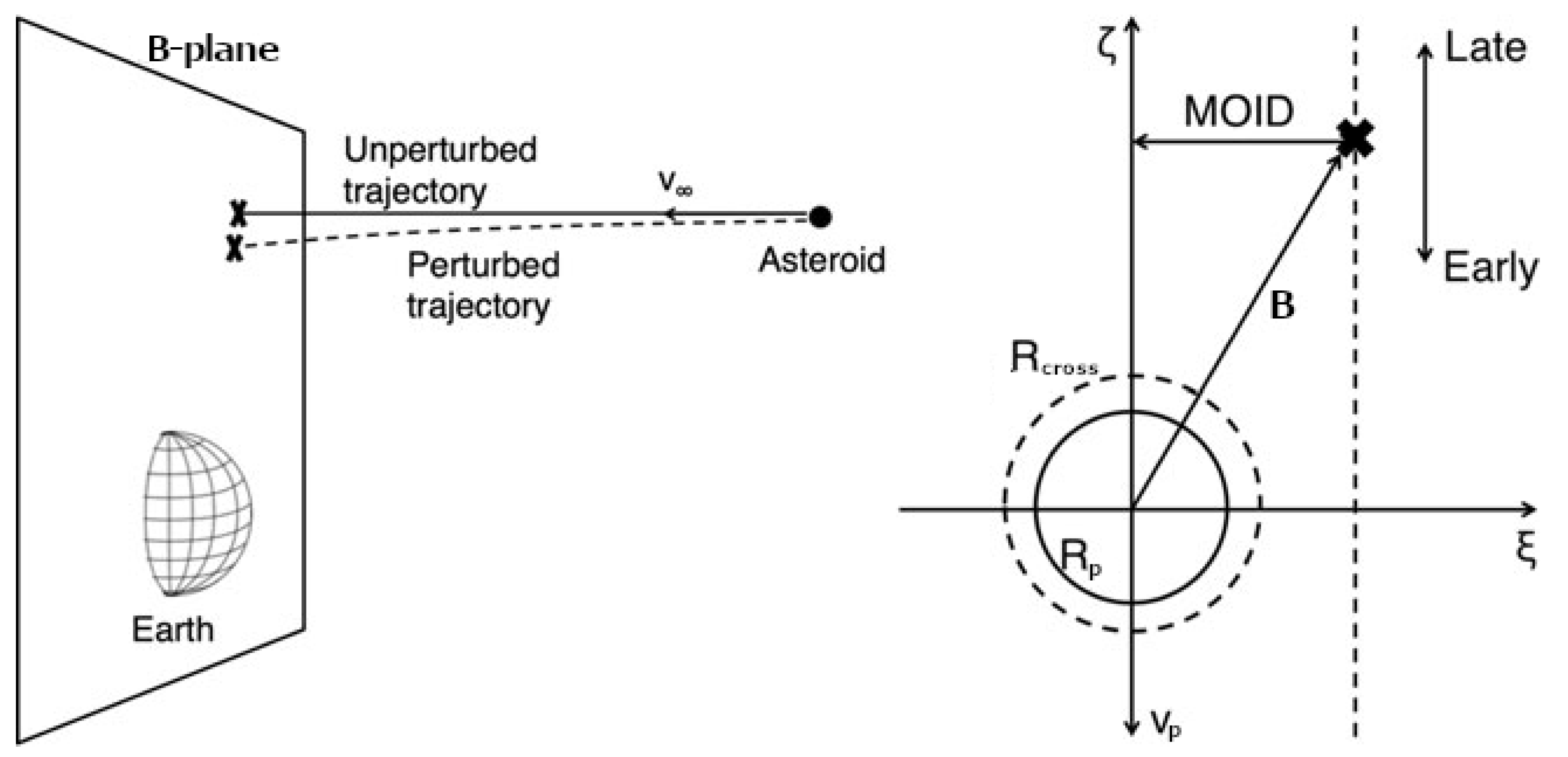
2.1. Target Planes
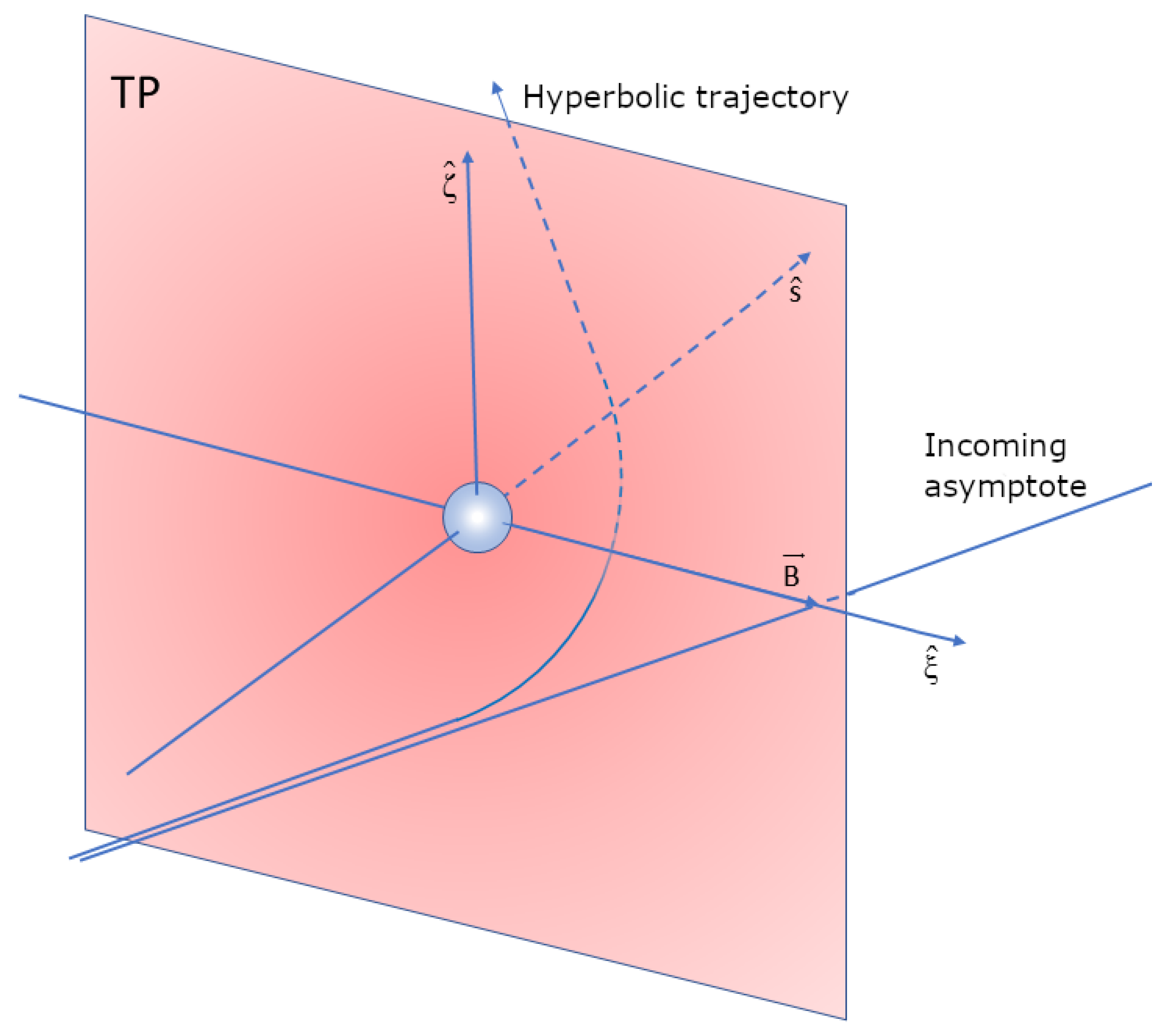
The geometry of a close approach can be described using the so-called Target Plane (TP) or b-plane (in the literature the impact parameter is also indicated with uppercase letter
B, e.g., in [
41]), a plane passing through the center of the Earth and orthogonal to the incoming asymptote of the hyperbolic geocentric orbit of the asteroid (see
Figure 1). The orbit of the small body is then completely described by a set of elements that includes two coordinates (
,
) on the TP, two angles (
,
) describing the orientation of the plane, the size
U of the escape velocity and the time
of the encounter (see
Figure 2). The impact parameter
b is the distance of the position of the object on the TP to the origin:
. In this way the encounter can be modelled as a planetocentric two-body scattering event.
Following [
42], if we use a geocentric reference frame
(the
Y-axis coincides with the direction of motion of the Earth, the Sun is on the negative
X-axis and the Earth is considered on a circular orbit around the Sun) then the components of the unperturbed geocentric velocity vector
of the small body with respect to Keplerian elements are (a system of units such that the distance of the planet from the Sun is 1 and the period of the planet is
is used):
The planetocentric velocity is
where
T is the
Tisserand parameter with respect to the planet
The angles
and
defining the direction of the incoming asymptote are defined as
and, conversely
As explained in [
41,
43], the
direction is oriented opposite to the projection of the heliocentric velocity of the Earth on the TP, thus is related to the along-track position of the NEO. This means that the coordinate
contains the information about how early or late the minor body is with respect to the encounter with the planet. The
direction is defined as
and its module
approximates the MOID. A schematic representation of the reference frame is reported in
Figure 2.
In this formalism, an
impact can be defined as an intersection between the asteroid trajectory and the cross section of the Earth on the TP, represented by a circle of radius
greater than the actual radius
of the Earth by a factor that accounts for gravitational focusing. The asymptotic velocity
U of the NEO for
is computed, as in [
41], from the conservation of energy:
As an alternative to the TP, a planetary encounter can also be described by means of the Modified Target Plane (MTP), passing through the centre of the Earth and orthogonal to the velocity
of the NEA at the time of closest approach ([
13]). Anyway the use of the TP provides an advantage with respect to the MTP, since gravitational focusing introduces a nonlinear deformation in the vicinity of an impact, thus the direction of
can vary greatly in a small uncertainty range. This implies that it might not be the same for all of the VAs that belong to the same object. On the other hand, the direction of
is unaffected by the encounter, since the incoming asymptote does not change, allowing representing all the VAs on the same TP. The MTP is mainly used in the frame of the imminent impact problem, where the gravitational focusing does not affect so much the VAs orbits (see
Section 5.2).
In its original formulation, Öpik’s theory of close encounters did not use a complete set of state variables. In the extension presented in [
28] a complete set of elements is introduced:
U,
,
,
,
and the time
of the ecliptic crossing by the small body. These variables are not canonical and in [
44] the author proved that a set of canonical variables containing some information about the position of the object on the b-plane does not exist.
2.2. Consequence of the Encounter
The effect of the close approach is the rotation of
into
, aligned with the outgoing asymptote, without changing the length:
. The angle
of deflection between the two vectors depends on
U, the mass of the Earth
m, and the impact parameter
b (
needs to be small to apply Öpik’s theory):
The angles
and
, defining the direction of the post-encounter velocity vector
, can be obtained in terms of
,
,
,
(this last angle is the polar angle on the TP which specifies the position of the small body) by
2.3. Resonant Returns and Keyholes
Using the units introduced before, the orbital period of the Earth is
, and that of the asteroid after the close approach is
. If the two periods are commensurable, that is
with
h and
k integers, then after
h periods of the asteroid
k periods of the Earth have elapsed, and both the Earth and the small body will be back again in the same position of the previous encounter. Such a subsequent encounter is called a
resonant return. Also if the ratio of the period is not exactly
, but is close, a subsequent encounter can take place, but the Earth will be earlier or later for the encounter than it was at the previous one. The new close approach conditions can be computed analytically and all the computations can be found in [
28].
An important advantage of an analytical, albeit approximate, theory of planetary close encounters is that it gives us a key to understand the divergence of orbits due to repeated close planetary encounters, enabling the study of chaotic phenomena. It also give the possibility to study in a simple way the chance of collision of a minor body with the Earth. The key concept is that of
keyhole. Such term has been introduced by Chodas ([
45]) to denote the small regions of the
b-plane of a specific close encounter such that, if the asteroid passes through one of them, it will hit the planet at a subsequent return, i.e., a keyhole is simply one of the possible pre-images of the Earth’s cross section on the
b-plane. The expression keyhole may also be used to indicate a region on the
b-plane leading not necessarily to a collision, but to a very deep encounter. Thus, a keyhole is tied to a specific value for the post-encounter semimajor axis
, i.e., to the value allowing the occurrence of the next encounter at the given date. The analytical description of a keyhole is quite simple as well as its geometrical representation on the TP (see [
28]).
3. Observations
The process by which a NEO is discovered and its orbit determined starts with observation, that is the recording of the position of an object on the celestial sphere, in order to acquire astrometric information. Depending on the kind of telescope used for the detection, the observation can be of optical or radar type.
An optical observation gives the position of the object in the sky using two angles, usually right ascension (indicated with RA or ) and declination (DEC or ). Optical observations also allow measuring the apparent magnitude through photometry.
Radar observations require the vicinity of the object to be performed successfully, since the signal to noise ratio for a target at distance r is proportional to . The advantage is an increase of accuracy in the astrometry, with respect to the optical case. The information provided by radar observations includes astrometry in terms of range and range rate with respect to the observer’s position, but also shape, size and rotational state of the object.
Observations are performed all around the world both by professional institutions and amateur observers, and are then submitted to the MPC, which is responsible for the designation of minor bodies in the solar system (according to the precepts dictated by the IAU) and for the efficient collection, computation, checking and dissemination of astrometric observations and orbits for asteroids and comets. Newly observed objects waiting to be confirmed as NEAs are posted on the NEOCP with a temporary designation until a reasonably reliable orbit becomes available. The page can also generate rough ephemerides for the objects in the list to facilitate the observers in their follow-up.
3.1. Surveys
A
survey is a project aiming at collecting observations for the largest and most representative sample of objects possible. The need for a NEO survey, aimed at the establishment of a complete catalogue of the Earth-threatening objects, was addressed for the first time in 1992 by NASA through a workshop establishing the
Spaceguard project ([
46]), with the goal to identify at least 90% of all NEOs with diameter greater than 1 km by the end of 2008. An international foundation with the same name, dedicated to planetary defense from impacting small bodies, was established in 1995, when
Spacewatch, the first telescope network dedicated to NEOs, was built and became operational. Since then, firstly to achieve the Spaceguard goal, then to reduce the completeness diameter as much as possible, numerous surveys have been conducted, and their results in terms of numbers of objects discovered are shown in
Figure 3.
The main ones are Spacewatch, LINEAR (Lincoln Near-Earth Asteroid Research), NEOWISE (formerly Wide-field Infrared Survey Explorer) and Pan-STARRS (Panoramic Survey Telescope and Rapid Response System). A brief description of their peculiarities can be found in [
47].
3.2. The Fly-Eye Telescope
Currently under development, the NEOSTEL Fly-Eye telescope is a new instrument expected to discover NEOs up to apparent magnitude 21.5, thanks to its wide survey observing strategy. The large field of view (6.7° × 6.7°) will allow scanning 2/3 of the visible sky three times per night and detect objects candidate for hitting the Earth a few weeks or days in advance of impacts. In other words, once the Fly-Eye will start operations, we expect an increment in the number of imminent impactors (see
Section 5.2). This will require an update of the currently available orbit determination methods and tools to improve the results in cases whose time span between discovery and possible impact is very short.
The first Fly-Eye telescope will be located in the site of Monte Mufara (Palermo, Italy) and will represent the core of the NEO optical observation network that ESA aims to build in the frame of its Space Situational Awareness (SSA) programme. The Fly-Eye telescope is named after its innovative core optics, consisting of a configuration of 16 distinct beams, the outputs of which recombine to form a large field of view image of the sky, similar to how the eyes of a fly work. The 16 optical channels are equivalent and, although independent of each other, share a common spherical primary mirror. The modularity of the structure allows for the channels to be added progressively, with no need to modify the already operational ones. Thanks to this characteristic, the deployment of the telescope could be split in two phases, the first of which led to the building and factory testing of an already functional instrument capable of observing half of the total field of view (ref. [
48]). In the second one, the structure with the remaining eight optical channels, will be completed and the installation at the selected final location performed. The architecture of the telescope consists of three main structures: the primary mirror, a centre piece and the secondary structure hosting the optical channels. The secondary structure is composed by the Central Beam Shaper (whose core part consists of a 16 facets beam splitter), the 16 optical tubes and a mechanical system for alignment of the secondary elements and the overall telescope structure. A state of the art CCD image-recording element is placed on the focal plane of each optical channel. To reduce the effect of thermal noise, each CCD sensor is operated in a vacuum chamber and kept at −50 °C by means of a Peltier electric cooler. Furthermore, NEOSTEL will be provided with a low-noise equatorial mount, allowing fast repositioning and damping of every vibration prior to image acquisition.
The location chosen for the first Fly-Eye telescope is atop the 1865 m a.s.l. Monte Mufara in Sicily, where a dedicated seeing monitoring system, provided with a meteorological station has been installed to collect statistical information about the expected observing conditions. In the building of the dome that will host the telescope, special attention is being paid to elimination of any temperature gradient that might affect the acquired images. In an estimation by means of a Monte Carlo simulation, the telescope is expected to detect 2.8 impactors per year (allowing 365 clear nights per year, thus clearly an overestimation). The number is expected to rise to 4.1 detections per year after the implementation of a second telescope, which is planned to be installed in the southern hemisphere.
3.3. Discovery
Moving objects are often discovered comparing several digital images of the same portion of the sky, taken in a time interval of 15 min to 2 h (a method used to detect transients in general, known as
blinking), singling out the objects that change their position with respect to the stars in the passing from one image to the next. A collection of astrometric measurements obtained from images that could correspond to the same moving object is called a
tracklet. Tracklets are then compared and linked, when possible, in order to obtain enough information to compute an orbit. We define a Too Short Arc (TSA) as an ensemble of one or more tracklets that does not contain sufficient information to calculate curvature, which is assumed to be significant if
where
is the
proper motion of the object and
is the
geodesic curvature of its path as a function of the derivatives of
and
with respect to the arc length
s, which is a parameter defined by
. The normal matrix
is the inverse of the covariance matrix
. Thus, this definition of TSA depends on the choice of the control value
.
Given
N chronologically consecutive TSAs, they can then be combined to form an
arc of type N if each couple of consecutive TSAs, once joined, shows significant curvature. By this definition, observations of NEOs taken on a single night often form an arc of type
, sufficient to compute an orbit. According to the definition given in [
49], a new object is
discovered when three requirements are simultaneously fulfilled for the first time:
an arc of type is available for the object,
a Least Squares (LS) orbit is computed and it fits the observational data with residuals compatible with the current error model,
enough photometric information to compute the absolute magnitude is available.
4. Managing the Orbital Uncertainty
The main problem to address in IM is the management of the uncertainty deriving from the observations and the orbit computation. In particular, when a small body has just been discovered, the preliminary orbit is poorly constrained because of the observations span only a short arc. There are cases where is possible to apply a LS method and to converge to a
nominal solution; but also orbits near the nominal one could be acceptable as solutions, because they have a Root Mean Square (RMS) error of the residuals not significantly above the minimum. The best method to represent this situation is to define a CR or
uncertainty region in the 6-dimensional space of orbital elements: an orbit belongs to the CR if the
penalty (increase in the target function with respect to the minimum, see
Appendix A for more details) does not exceed some threshold depending on the parameter
.
Many applications, including the one we are interested in this paper, require the use of the entire set of orbits belonging to the CR. Since the N-body problem, that is the basic dynamical model for asteroids, is not integrable, it is not possible to obtain all the orbits for some time span in the future or in the past. The only thing to do is to compute a finite number of orbits by numerical integration.
The CR is sampled by a finite number of VAs, ranging between a few tens and a few tens of thousands, depending on the application and on the available computing power. It is possible, and in some cases it is achieved, to select the VAs at random, as the so-called MC methods do. However, the idea developed at the end of 1990s was to consider a geometrical object, the
Line Of Variations (LOV), a one-dimensional segment of a curved line in the initial conditions space. There are several different ways to define, and to practically compute, the LOV, but the general idea is that a segment of this line is a kind of spine of the CR. In [
5] the LOV is seen as a solution of an ordinary differential equation with a vector field defined by the weak direction (the direction of the eigenvector of the normal matrix relative to the smallest eigenvalue) and considering the nominal LS solution as initial condition. This kind of definition is not stable, in particular when there is a largely dominant weak direction, which is precisely where the LOV is most useful. To face this problem, a corrective step in the algorithm was introduced, using differential corrections constrained on the hyperplane orthogonal to the weak direction. In this way an approximation of the LOV can be computed in a stable manner. This algorithm, called
constrained differential corrections, is useful also to define the LOV as set of points of convergence ([
9]). Doing so, the definition corresponds to the numerically effective algorithm implemented for the sampling of the LOV. Furthermore, this definition can be used also when the nominal solution either does not exist or has not been found. The algorithm described naturally samples the LOV, generating a certain number of VAs equally spaced in the parameter used to define the curve (usually this parameter is called
). As said, in recent years, the possibility to sample the LOV with constant steps in probability, considering a Probability Density Function (PDF) on it, has been introduced ([
10]).
The dynamics of the LOV points is very interesting because they are in order. For example, if in the time span between the time of initial conditions and that of prediction is long, but strong perturbations (e.g., planetary close encounters) are not experienced, then the VAs will stay approximately uniformly spaced as at the initial time. If close approaches occur during the time of propagation, the prediction can become much more difficult.
Another kind of problem arises when the observational data are poor, for example due to too few days of observations. In this case the CR has a two-dimensional structure and the selection of a LOV is quite arbitrary because of a strong dependence on the coordinates used for the preliminary OD. The best strategy to face this situation is to sample the CR using different LOVs (it is possible to exploit the other directions defined by the eigenvectors of the normal matrix) or using a two-dimensional sampling, as described in the next subsection.
4.1. The Admissible Region
In the last 20 years there has been a huge increase of observations classified as Too Short Arcs (TSAs): a TSA is a set of observations which span a too short arc on the celestial sphere to perform a full OD (full means arriving to a LS solution). In [
19], the authors started to face the problem of the existence of large databases of TSAs. In particular, they identified a TSA using an
attributable, a set of four quantities (two average angular coordinates and two corresponding angular rates) at a reference time (usually the mean of the observing times). The attributable is computed using a linear regression or a polynomial fit on the observations detected and therefore leaves undetermined the radial geocentric distance of the object
r (
range) and its time derivative
(
range-rate). However the attributables are sources of useful information and in order to exploit it the Admissible Region (AR) has been defined: it is a compact region in the
plane, over which is possible to define a 2-dimensional manifold, the Manifold Of Variation (MOV, see
Section 4.2). Sampling the AR by
Delaunay triangulation allows to consider the nodes as VAs with a two dimensional structure. In [
15] the idea to use this structure to search for VIs has been explored, but the feedback has been negative: after a propagation, the resulting structure was too complex to perform a significant analysis. However, the idea of a 2-dimensional manifold, the so called
Manifold Of Variations (MOV), will come in handy for the problem of imminent impactors (
Section 5.2).
Now, let us introduce the fundamental concepts of attributable and AR. Let us consider an asteroid, at time t, with a heliocentric position P and observed from the Earth, which is at the same time in . Then let be spherical polar coordinates for the geocentric position .
Definition 1. An attributable is defined, at a time t (the mean of the times of the observations), as a set of four quantitiesobtained by a polinomial fit starting from the available observations. The reference system defining the angles can be an equatorial reference system (e.g., J2000), so the angles are the right ascension for and the declination for , or an ecliptic system, but the equations defining the AR do not change. The information on the average apparent magnitude h, if available, can be attached to the attributable. The range r and the range rate are left undetermined by the attributable, but we can extract information using the hypothesis that the asteroid belongs to the solar system, but not to the Earth-Moon system. To constrain the range and the range-rate and to define a compact region in the plane the following quantitites are used: the heliocentric two-body energy , the geocentric two-body energy , the radius of the sphere of influence of the Earth and the physical radius of the Earth .
Definition 2. Let us suppose to have computed an attributable from a TSA. The Admissible Region (AR) associated to the attributable is the domainwhere - (A)
( is not a satellite of the Earth);
- (B)
(the orbit of is not controlled by the Earth);
- (C)
( belongs to the Solar System);
- (D)
( is outside the Earth).
In [
19] the authors found analytical formulas based on the Definition 2 and they proved that the AR consists of at most two connected components, and that it is compact being the inside of a finite number of closed continuous curves. Once the AR is defined, we can sample it (by a grid or by triangulation) and each node defines the orbit of a VA, expressed as (considering, for example, that the angular coordinates are right ascension and declination)
where
and
. Such elements are called
attributable orbital elements and we have to assign them an uncertainty. This case is quite different from the usual one because a
covariance matrix is not available. Thus, the CR describing the uncertainty of
can be defined by
where
is a parameter,
is the nominal (least squares) value of the attributable angular coordinates, and
is the corresponding normal matrix. This set is not a Cartesian product, although in many cases it can be approximated by the Cartesian product of a confidence ellipsoid in the
A space times the AR computed with the nominal attributable
:
The
quasi-product structure of Equation (
7) and its approximation with the product of Equation (
8) play an important role in the process of prediction of future/past observations with a formal uncertainty and in the process of identification, as described in [
50].
4.2. The Manifold Of Variations (MOV)
Very Short Arcs (VSAs) are sequences of observations closely spaced in time, assumed to be of the same physical object and with which it is possible to compute preliminary orbits with their own uncertainty. Giving a look to the eigenvalues of the covariance matrices of the preliminary orbits we can note that frequently there is not a predominant eigenvalue, but there are two eigenvalues much bigger than the others. This means that there is not just one direction of uncertainty and the CR has a 2-dimensional structure. Therefore, as already anticipated, it is not sufficient anymore to sample one LOV: it could be possible to compute several LOVs in different coordinates and then to go on with the methods already explained, but it is more reliable to change the geometrical object used by switching to a sampling by surfaces.
The idea is to construct a
cobweb covering the CR in the plane
using the level curves of the cost function used to minimize the RMS of the observational residuals. For each level curve, points corresponding to some fixed directions are selected and used as VAs. Let us show how to do this construction starting from a least square solution and its uncertainty (as described in [
26]), represented by a
covariance matrix. We initially create a regular grid of points (the nominal solution is, for simplicity, fixed in
) in the space of polar elliptic coordinates
, where
and
(
is a parameter defining the maximum value of RMS that we consider reliable in our analysis). Then we apply to each point of the grid the transformations described below, depending on the covariance matrix of the preliminary orbit and on the orbit itself.
We switch from the grid in the space
to the range/range-rate plane using the map
where
and
are the eigenvalues of the
covariance matrix of the variable
and
is the eigenvector corresponding to the greater eigenvalue
.
Since we have assumed that the nominal solution is in the origin of the range/range-rate plane, we have to move all the points by the vector
, that represents the real position of the the preliminary orbit computed with a least square fit:
Figure 4 shows the cobweb sampling of the CR of asteroid 2004 FU
with the first 17 observations. The variables are
(corresponding to the maximum value of
R), the number of directions computed and the number of points in each direction.
Since the orbits computed in this way are not so accurate we apply a differential correction along each direction. Let us fix a direction h in the the plane and let us describe the recursive method applied:
- 1.
we start from the 6-dimensional preliminary orbit composed by a 4-dimensional vector of elements and by the projection on the plane;
- 2.
we consider the next point in the plane along the fixed direction and we construct the orbit ;
- 3.
we apply a differential correction constrained to the 4-dimensional vector obtaining a new vector which gives us a new orbit corresponding to the point ;
- 4.
we repeat the previous steps analyzing all the points along the direction h.
We apply this procedure for each direction generating a set of 4-dimensional points
which constitute a 4-dimensional manifold parameterized by the 2-dimensional cobweb. We shall call this manifold the
Manifold Of Variations (MOV). A formal definition of the MOV can be found in [
27]:
Definition 3. Given a subset K of the AR, we define the Manifold Of Variations to be the set of points such that and is the local minimum of , when it exists.
5. Impact Monitoring Overview
As seen in the previous section, the observational data provide a set of possible orbits, but we do not know which is the real one. All these orbits belong to the CR; the goal of IM is to establish if the CR of a given NEO contains a small subset of initial conditions leading to a collision with the Earth (what we called VI). The collisional subset for a given epoch may be disconnected, for example when the same collision can be reached in different dynamical ways; in this case a VI is a connected component of the collisional subset. The Impact Probability (IP) of a VI is roughly proportional to the volume of the VI in the elements space. To find an initial guess belonging to the VI, the VI representative, when the IP is very small, it is necessary a very dense sampling of the CR. The current classical impact monitoring systems, CLOMON2, Sentry and AstOD use the LOV as a tool to sample the CR. While Scout, NEORANGER and NEOScan use the MOV. In this section we will describe the methods and the algorthms to search for VIs used by the classical IM systems and by the systems developed for the imminent impactors.
5.1. Classical IM
The goal of IM is to find VIs and to alert the astronomical community of a potential risk. The first thing to do when we are searching for VIs is to explore the CR sampling the LOV (see
Section 4) and obtaining an ordered set of VAs (also called multiple solutions). Unfortunately such sampling is dependend on coordinate system, that is the multiple solutions obtained depend on the coordinates used for the preliminary OD. The IM systems have the possibility to investigate different coordinate systems. CLOMON2 and AstOD usually use Equinoctial elements, but also run in Cartesian coordinates; Sentry uses Cometary elements but can optionally run in Cartesian or Keplerian. If the arc is short, Cartesian coordinates are preferable.
Once the LOV has been sampled, each VA is propagated to some point in the future (typically 100 years after the discovery), recording all the information about the close approach. For each encounter, the goal is to find, among the LOV points, the minimum possible approach distance. This task can be done performing a minimization of a function of one variable , the closest approach distance (around a given date) squared, as a function of the parameter along the LOV. The function is differentiable, therefore it is possible to search for zeroes of the derivative . If there is a closed interval such that a close approach occurs (to the Earth and around the same epoch) for all initial conditions corresponding to a parameter , and the values of the derivative at the two extremes are and , then there is at least one minimum of inside the interval. If the previous conditions are satisfied, the regula falsi algorithm provides an iterative procedure converging to some stationary point (almost always a minimum).
This approach is quite simple, but two problematic scenarios can appear. First, in order to start such algorithm we need at least two consecutive VAs with encounters around the same date, thus tracing two sequential points on the same TP. Second, the minimum possible distance along the LOV could be more than one Earth radius and still an impact could be possible, because the image on the TP of the entire CR is not just a line but has some width.
The case of one only TP point is called
singleton: the solution is to use a unidimensional Newton’s method or a densification around the point ([
51]). CLOMON2 and AstOD implement a variant which searches for zeroes of
with controlled length steps, in such a way that divergence is not possible, provided that the image on the TP exists for some neighborhood of the first LOV point. Nevertheless this method can fail because of strong nonlinearity. Sentry ignores singletons applying densification in such cases.
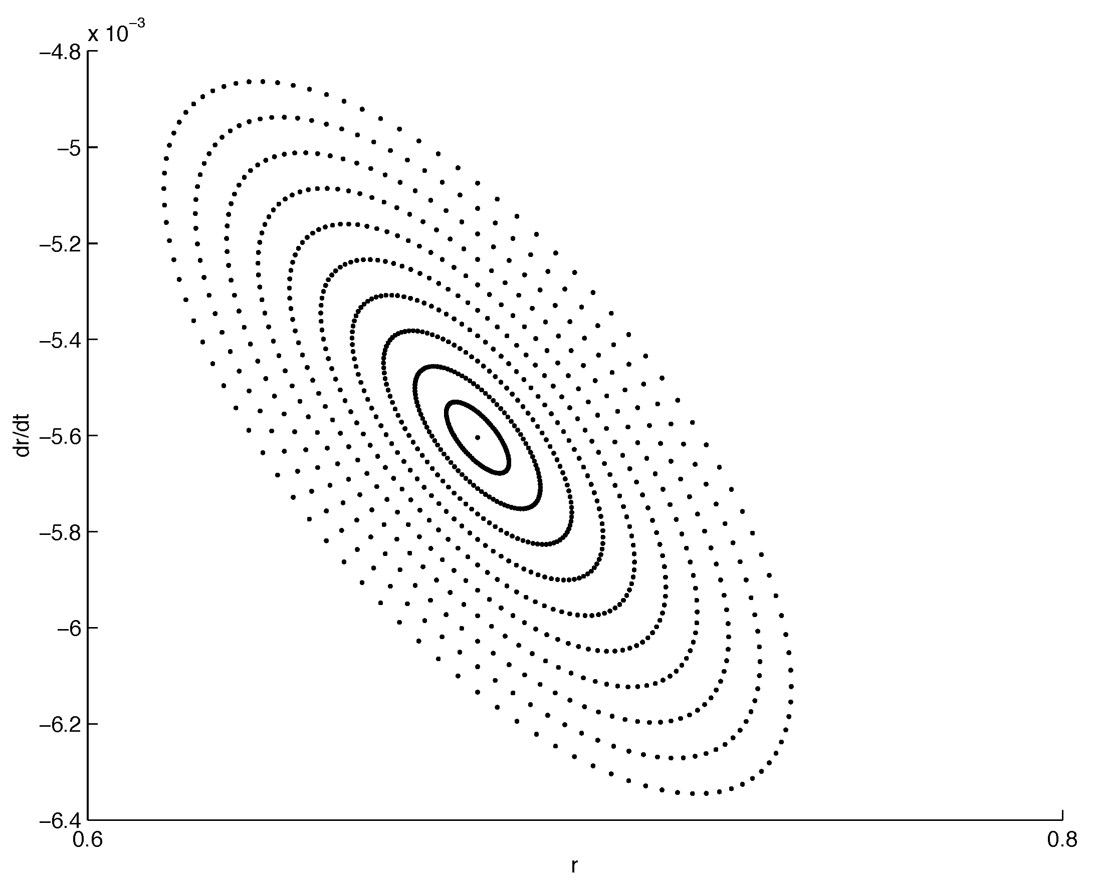
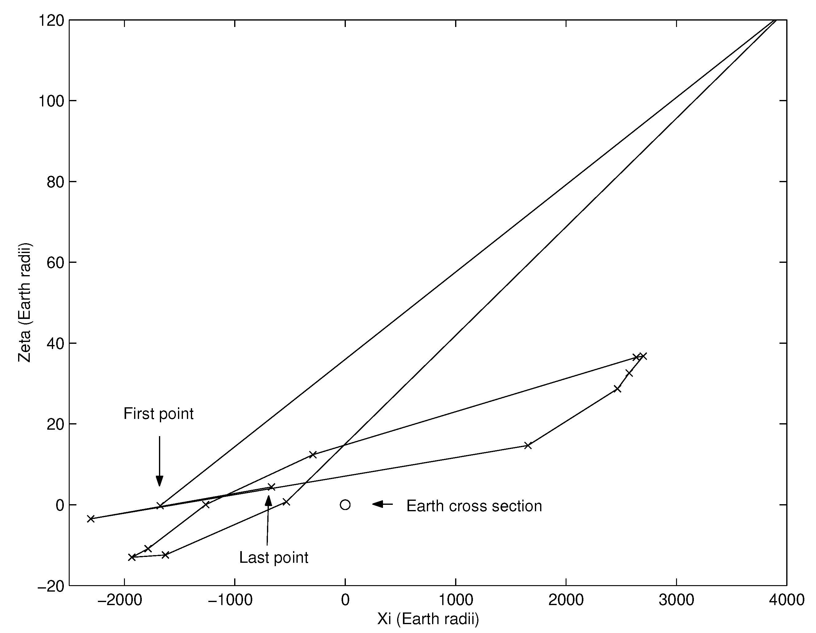
CLOMON2 and AstOD algorithms use the so-called
principle of the simplest geometry, by which we suppose that the qualitative behavior of the LOV image on the TP is the simplest possible with the available information on the TP points. Subsequent close encounters make this behavior more complex with no absolute limit on the complexity of the figure drawn by the LOV on a TP:
Figure 5 shows a typical example of chaotic behavior. As in fractal sets, smaller and smaller subintervals on the LOV can be distorted according to a typical pattern. The principle of the simplest geometry allows the algorithms to stop within acceptable computation times by not following finer and finer details.
Once the minimum along the LOV has been found, we should show the existence of a VI, a connected region in the CR leading to an Earth impact at the given date. If it exists, we need to compute the associated IP. The TP point of minimum distance along the LOV could be outside the impact cross section of the Earth and nevertheless a VI could exist: this is because the image of the CR is not exacly a curve, but more like a 2-dimensional strip around it. The basic approach is to linearize the map between the initial conditions space and the TP; so the confidence ellipsoid in the initial conditions space is mapped onto an elliptic disk on the TP. If this disk intersects the impact cross section there is a VI.
To compute an IP, all the IM systems use the Gaussian formalism, starting from the hypothesis that the residuals are Gaussian random variables. Therefore a Gaussian distribution can be used to describe the set of initial conditions with the boundary ellipsoids of the CRs as level surfaces, and this distribution can be projected onto the TP obtaining a normal distribution (in two dimensions) with the above mentioned ellipses as level curves. The coefficients of the Gaussian distribution on the TP can be explicitly computed ([
13]) and a probability integral of this distribution on the impact cross section can be computed ([
14,
26]). Due to the nature of normal distributions (always positive) also for very distant close approaches, the IP would be positive; however, when the probability formally computed in this way is very small, e.g.,
, the VI is just rejected.
Given a point on the TP, , the uncertainty associated can be represented using an ellipse (projection of the confidence ellipsoid onto the TP) centered in the point. The semimajor axis is called stretching, while the semiminor axis w is called semi-width. To express the PDF in a more understandable way, a rotation of the coordinates by the angle between the major axis of the confidence ellipse on the TP and the axis is performed. The new rotated coordinates gives the possibility to express the PDF as the product of the two densities
, along the width direction,
, along the stretching direction.
Then the complete probability density is
and the probability of an Earth impact is
where
is the impact cross section on the TP (note that the disk has a radius
, larger than the physical radius of the Earth
, because of gravitational focusing). Obviously, it is not necessary to compute this integral where the PDF is negligible, so the integral can be computed over a finite TP domain with a maximum extension of
:
where
The results obtained with this modelling are reliable until two conditions are fulfilled: (i) the set of VAs obtained sampling the LOV is representative of the entire CR; (ii) the point of closest approach along the LOV has a small distance from the center of the Earth, so the linearization of the Gaussian PDF represents quite well the PDF at the Earth. However, such conditions can drop, especially when the observations are few and the uncertainty large. If the linearized Gaussian approximation fails, we can identify spurious VIs: they are cases in which the approximated IP is non-negligible, while an exact probability computation would give an actually vanishing result. The goal of IM is not to find all the VIs for a given object or to avoid all the spurious ones. The basic requirement is to obtain a list of VIs which is not empty when, and only when, the real list of VIs with non-vanishing probability is not empty. Doing so, the asteroid can be labelled as to be reobserved, and the new observations will allow recomputation. To face the problem of spurious VIs an algortihm has been developed. The spurious VI elimination algorithms of CLOMON2 and AstOD are based on the fact that in order to prove the existence of a VI the representative of the VI must be exhibited. These algorithms start from the TP point of the closest approach and apply a Newton method to obtain an initial condition leading to a TP point inside the impact cross section. If this iterative procedure fails, the VI is rated as spurious. If the procedure converges to an explicit VI, the IP is rescaled by using the RMS of the observation residuals; in practice, if the orbit of collision results in unacceptable residuals, the VI is also considered spurious. Sentry has a different approach with spurious VIs, testing for excessive nonlinearity at the point of closest approach to the Earth. If the LOV local behavior is highly nonlinear (considering the curvature of the LOV and the rate of change of stretching), then the VI detection is considered unreliable and discarded. This approach has the opposite problem with respect to those of CLOMON2 and AstOD, in the sense that some spurious VIs can be unfiltered. However, it is preferable to add to the list some spurious VIs than to eliminate a significant VI. Obviously, the risk of rejecting a real VI is present in all the approaches used, but such cases can be expected to have very small IPs due to the extreme nonlinearity.
Communication of the Risk
The
Torino impact hazard scale (TS) is a system designed to communicate to the public the risk associated with a future Earth approach by an asteroid or comet. This scale, which has integer values from 0 to 10 (0 means virtually no chance of collision, while 10 means certain global catastrophe), takes into consideration the predicted impact energy of the event and the impact probability. It has been adopted by a working group of the IAU in 1999 at a meeting in Torino ([
52]) and revised in 2004 ([
53]).
The
Palermo Technical Impact Hazard Scale (PS) has been developed by and for NEO specialists. The goal was to classify and prioritize potential impact risks spanning a wide range of impact dates, energies and probabilities. PS values less than −2 describe events without consequences, while PS values between −2 and 0 indicate situations that have to be monitored. VIs with positive PS values will generally indicate situations that merit some level of concern. The scale compares the detected potential impact with the background risk, that is the average risk posed by objects of the same size or larger over the years until the date of the potential impact. The scale is logarithmic: a PS value of −2 describes a potential impact event that is only 1% as likely as a random background event, a value of zero indicates that the single event is just as threatening as the background hazard, and a value of +2 indicates an event that is 100 times more likely than a background impact. The primary reference for the Palermo Technical Scale is [
54].
5.2. Short-Arc OD and Imminent Impactors
Short-arc OD indicates the capability to compute an orbit when an asteroid is first discovered. In such cases we are interested in a fast follow-up in order to exclude that the object could be an imminent impactor, which is an asteroidal object impacting the Earth shortly after its discovery, within the same interval of observability (apparition). The few observations permit to compute an attributable, but they leave almost unknown the range and the range-rate. We can infer information using the AR (see
Section 4.1) and some ranging methods alternatives to the MC ones. There are two possible approaches to the ranging methods: statistical ([
7,
8,
17,
55,
56]) and systematic methods ([
16,
18,
57]).
The original statistical ranging method ([
7,
8]) selects a pair of astrometric observations and, then, the right ascension and the declination are randomly sampled. Candidate orbital elements are included in the sample of accepted elements if the
-value between the observed and computed observations is within a pre-defined threshold and the sample orbital elements obtain weights based on a meticulous debiasing procedure. In [
55] the authors improved the statistical ranging by replacing the random sampling with the use of a PDF that produces a chain of orbital elements in the phase space. This method is called Markov-Chain Monte Carlo (MCMC) ranging method and it is based on a bivariate Gaussian proposal PDF for the topocentric ranges. Then, in [
56] the authors have developed a random-walk ranging method in which the orbital-element space is uniformly sampled, up to a
value, with the use of the MCMC method. The sample orbits obtain weigths from the
a posteriori probability density value and the MCMC rejection rate.
In [
16,
57] the authors introduce the so-called systematic ranging, which systematically explores a raster in the topocentric range and range-rate space. This technique provides a geometric description of the orbital elements as a function of range and range rate. Systematic ranging also allows to identify regions of the phase space filled with impact solutions and the corresponding impact times and locations.
In [
18] the authors introduce a new approach to the systematic ranging, based on the AR tool: in particular, the AR is scanned by a regular semi-logarithmic or by a uniform grid and the MOV is computed. If a preliminary orbit exists, the MOV is compute as in
Section 4.2 using a cobweb. Sampling the MOV, a set of orbits (VAs) compatible with the observations can be obtained and propagated into the future (usually 30 days from the date of the observations) looking for VIs using the MTP tool.
A probability distribution on the MOV can be defined in order to compute the impact probability associated to a given VI. The residuals
can be assumed Gaussian random variables with the following probability density
where
W is the weight matrix, and
m the number of observations. The choice of the weights for each observatory is fundamental, and it has to take into account the fact that the discovery observations are few and can sometimes not reach the precision usually assigned to the observatory itself.
The a-posteriori probability density function for
is given in as:
where
is a prior distribution on the sampled space. Some possible choices for the prior probability are the following.
Jeffrey’s prior. It has been used for the first time in [
58]. It takes into account the partial derivatives of the vector of the residuals with respect to the coordinates
. Jeffrey’s prior tends to favor orbits where the object is close to the observer, because of the sensitivity of the residuals for small topocentric distances.
Prior based on a population model. This approach requires the choice of a metric on the absolute magnitude that is not unit independent.
Uniform distribution. This choice can appear simplistic, but it identifies the potential impactors without particular problems.
The uniform distribution is a natural choice, because it represents a good compromise between a simple approach and the good identification of potential impactors. In [
18] a new algorithm to propagate the probability density function back to the sampling space without any
a priori assumption has been presented. It is based on the law of transformation of the Gaussian random variables and on the following spaces:
S is the space of the sampling variables. It changes depending on the case we are considering: if the sampling is uniform in , if the sampling is uniform in , whereas in the cobweb case.
is the subset of the points of the admissible region such that the doubly constrained differential corrections give a point on the MoV;
is the MoV, a 2-dimensional manifold in ;
is the residuals space. The residuals are a function of the fit parameters, that is , with a differentiable function, and we define the manifold of possible residuals as .
Then the following chain of maps is considered:
and their Jacobian determinants are used to compute the probability density function on
S. In particular, in the neighborhood of each point of the MOV, it is possible to compute the density coming from
V, and then to pull it back to
S. Let
be the variable of the sampling space
S, and let
be the corresponding random variable. Moreover, using the compact notation
to indicate
, the probability density function of
is
where
is the
matrix associated to
, and
is the
Jacobian matrix of
. The derivation of (
9) is given in the appendix of [
18].
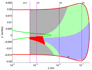
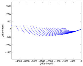
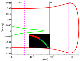
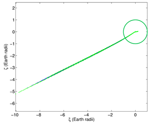
The Case of Asteroid 2018LA
This section is devoted to the analysis of an interesting case of imminent impactor. In 2018 the small Apollo-type NEA 2018LA was discovered by the Mt. Lemmon Survey. The object could not be detected before it came very close to the Earth due to its high entry velocity and small size (the estimated diameter was of a few meters). Only 8 h later, it impacted the Earth’s atmosphere over Botswana, becoming the third imminent impactor ever detected and the perfect opportunity to test the systems performing short term IM. Among these, we will focus on NEOScan.
In the following hours after the first observational data were published on the NEOCP, follow-up observations were performed and 4 tracklets were obtained. The results produced by NEOScan for each of these observed arcs can be summarized in a brief timeline:
09:04–09:18 UTC: first run over three observations (obs. time = 08:25 UTC), covering a time span of min. The absolute magnitude can be estimated between a minimum value and a maximum value , thus indicating a small object. The observed arc shows no significant curvature, so it is classified as type 1. Since no reliable nominal solution is available, the double grid sampling of the AR is performed, yielding a 5304 points MOV. The observation score ensures that the object is a NEA, while the estimated Impact Probability is . The object is declared nonsignificant, since the observed arc is shorter than 30 min, but is given impact flag 1, which produces an alert for the observers.
11:41–11:57 UTC: second run over 11 observations (obs. time = 09:07 UTC), covering a time span of 85.2 min, sufficient to declare the case as significant. The arc shows significant curvature and is classified as type 2, with geodesic curvature signal-to-noise ratio smaller than 3. Again, the AR is scanned via the double grid, but the corresponding MOV has reduced to 634 points, of which 168 can lead to an impact. The estimated Impact Probability rises to , leading to the assignment of impact flag 3.
14:10–14:26 UTC: third run over 12 observations (obs. time = 09:11 UTC), still covering a time span of 85.2 min. With a single additional observation, the software computes a MOV consisting of 584 points, of which 177 are possible impactors, thus increasing the Impact Probability to .
14:13–14:40 UTC: fourth run over 14 observations (obs. time = 09:40 UTC), covering a time span of 226.8 min. The tracklet becomes an arc of type 3, allowing for the computation of a reliable nominal solution with RMS = 0.571. The new estimate for the absolute magnitude is . NEOScan performs a cobweb sampling of the AR, that results in a 8811 points MOV, each of which is an impactor, therefore Impact Probability rises to .
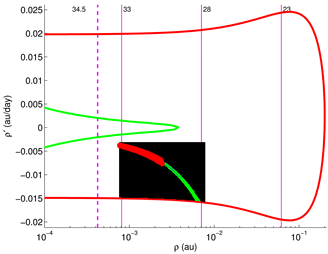
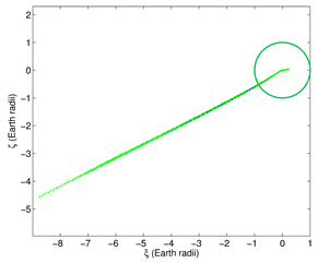
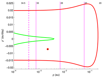
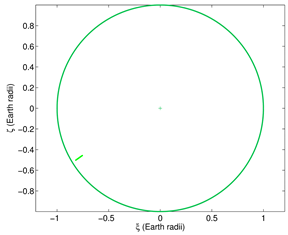
The AR and MTP projection evolution for each tracklet, with the consequent Impact Probability value, is shown in
Table 1, where in the AR representation, the legend is as follows:
the red solid line identifies the outer boundary;
the green dashed line shows where the geocentric energy is equal to 0;
the magenta dashed line represents the shooting star limit condition;
the magenta solid lines represent different values of the absolute magnitude;
dots representing VAs are indicated in blue if , green if and black if ;
red dots correspond to VIs.
Table 1.
Evolution of the IP, AR and MTP projection for each tracklet obtained for 2018LA. Figures from [
60].
On the MTP projections, the Earth’s cross section is indicated by the green circle centred in the origin.
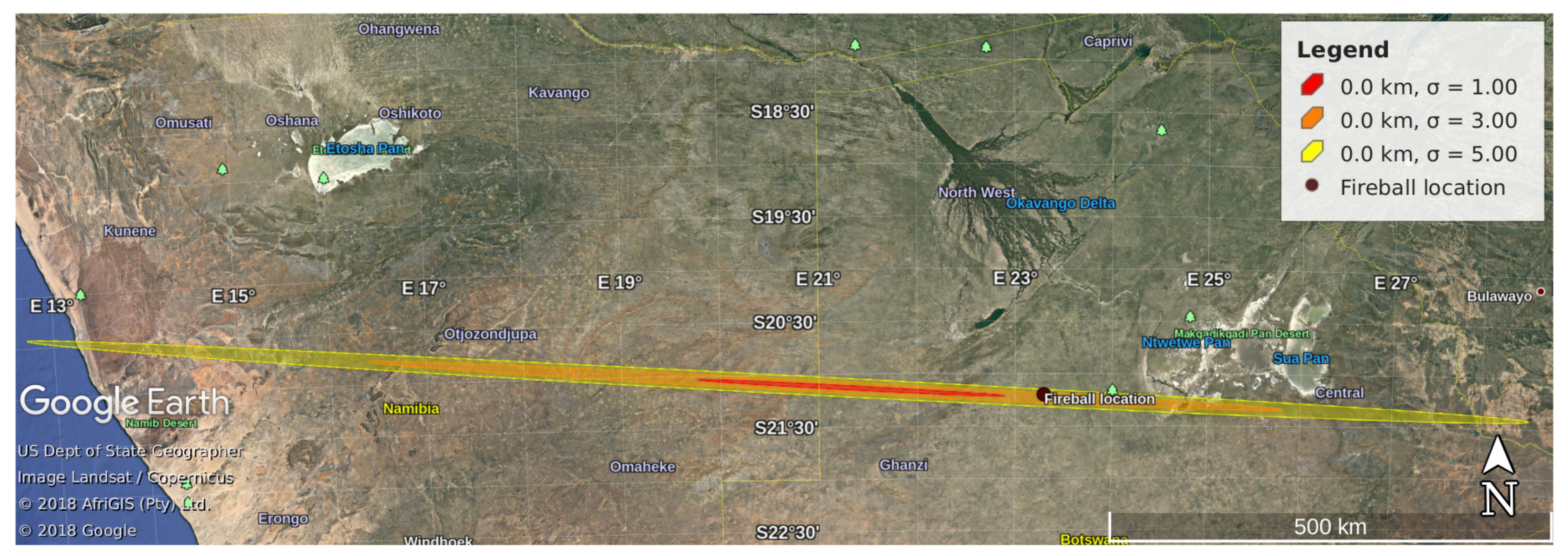
Once the collision is certain, the last step, in order to identify the potential impact locations and adopt the necessary safety measures, is the prediction of the impact corridor. This is done by means of the
semilinear method ([
59]) consisting of a mapping from a representative curve on the boundary of the confidence ellipsoid to the target two-dimensional space of geodetic coordinates. A representation of the resulting corridor for 2018LA is shown in
Figure 6.
6. Future of Impact Monitoring and Conclusions
As already discussed and explained in [
60], at the moment there are two types of automatic systems dealing with IM of NEOs:
- (1)
those for already designated orbits, such as CLOMON2, Sentry and AstOD, and
- (2)
those for the detections of imminent impactors (SCOUT, NEORANGER, NEOScan).
Systems of class (1) use data from MPEC, and a geometrical sampling of the CR with the LOV, while those of class (2) scan the NEOCP and use systematic ranging methods and/or geometric sampling with a 2-dimensional manifold.
The birth of these two classes of systems has been essentially dictated by the history of searching for NEOs, by the grow of observational facilities and by the amount of data available. When CLOMON2 and Sentry started their activities, the scientific and public communities were interested in big objects that could have caused global damage, while at the moment, the attention has moved to small objects and meteoroids ([
61,
62]). Probably, the differentiation in this two classes are due also to the rules of the MPC, or better, how the automatic systems catch the data from it. In this processes there could be a flaw, in the sense that there are objects, with a very well-defined orbit, remaining on the NEOCP, and, on the contrary, there exist designated objects with a great uncertainty. Thus, there are a certain number of cases that are not properly processed: object with a very well defined orbit should be processed like ordinary cases using, for example, LOV methods, while designated objects would deserve a treatment using a different sampling of the CR.
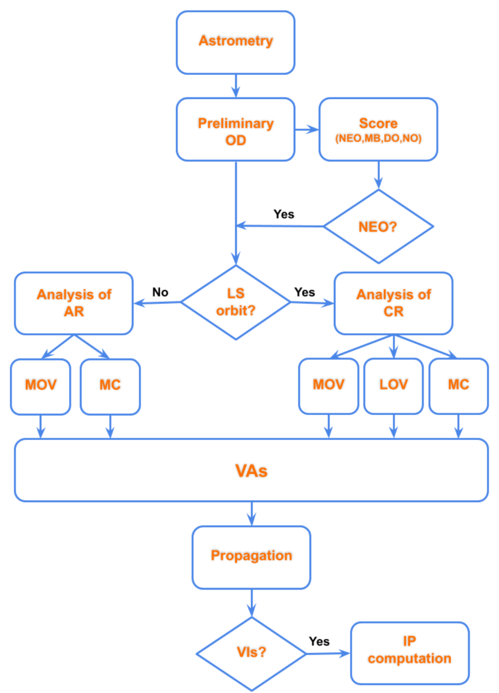
An idea to overcome this criticality, which could expand in the future with the advent of new technologies, could be the development of an
unified system (see
Figure 7).
This kind of system should start from NEOCP data of an object, decide the type of orbit and which is the best possible algorithm of OD to extract as much information as possible. The starting step should use, for example, the NEOScan algorithms to give a first insight to the observational data and to understand, using the score of the detection, the type of orbit. The score is the probability that an object belongs to the classes listed below:
NEO, Near-Earth Object, an object with perihelion distance ;
MBO, Main Belt Object, an object belonging either to the Main Belt or to the Jupiter Trojans; in particular, it has to fulfill the conditions
where
a is the semimajor axis (in AU) and
e is the eccentricity;
DO, Distant Object, characterized by (for instance, a Kuiper Belt Object);
SO, Scattered Object, not belonging to any of the previous classes.
In case the probability of being a NEO is greater than some threhsold, the algorithms for searching VIs should start. The choice of the more convenient algorithm should be based on some facts and quantities:
Knowing the previous input, the system should be able to decide:
- (a)
the way to sample the uncertainty region (AR or CR);
- (b)
the duration of propagation;
- (c)
how to detect potential impactors after the propagation and the projection on the TP of an encounter;
- (d)
in case of an impact detection, how to compute the impact corridor and the potential damages on Earth.
Concerning (a), a possible improvement is the use of a MC sampling of the CR, when a nominal solution exists. MC method starts from a given probability distribution of initial conditions and propagated forward in time while recording the number of impacts. This kind of method has the advantage of making no simplifying assumptions on how the orbital uncertainties are mapped into the future. However, the MC method is a very computationally expensive technique because it requires propagating a large number of VAs, typically of the order of the inverse of the target probability resolution. However, due to increase in the speed of processors, new MC-type methods are being studied ([
63]) in order to replace geometrical sampling. A new automatic system, as we have in mind, should have the capability to use both a geometrical sampling or MC method and above all understand when to use one and when the other.
In conclusion, the IM of Near-Earth Objects (NEOs) is a fascinating field of research that involves astronomy, mathematics and computer science: the mathematical algorithms evolve in time because they have to follow the progress in the hardware and software stuff (e.g., observatories, computers).
In this paper, I tried to summarize the last 25 years of work in the field, highlighting the main algorithms to find potential Earth impactors, and I gave an insight to possible future developments. In reality, there is another aspect that could be investigated: the possibility of using Machine Learning (ML) and/or Deep Learning (DL) approaches to the problem; but this is material for the next decade.


