Near-Earth Asteroid Capture via Using Lunar Flyby plus Earth Aerobraking

Abstract

Capturing Near-Earth Asteroids (NEAs) in the Earth-Moon system is a potential method of future space exploration and resource utilization. In order to make the captured NEA easily rendezvoused by spacecrafts, it is expected to capture the asteroid in a low-energy and low-inclination orbit. Lunar flyby and Earth aerobraking have been proved to be effective energy-saving methods in asteroid retrieval missions. Based on the Earth aerobraking capture strategy, if a lunar flyby process is performed before the asteroid enters the atmosphere, the thermal ablation of the asteroid in the atmosphere is expected to be alleviated. This paper proposes a lunar flyby plus Earth aerobraking method to capture an NEA. Using Geostationary Transfer Orbit (GTO) as the target orbit, the efficiency of three different capture strategies (direct capture strategy, Earth aerobraking capture strategy and lunar flyby plus Earth aerobraking capture strategy) are compared. Compared to the Earth aerobraking capture strategy, simulation results show that the main advantage of the lunar flyby plus Earth aerobraking capture strategy is that the mass loss ratio can be reduced (15 real asteroids are used as examples and mass loss ratio can be reduced by 0.98–3.39%). For example, for an asteroid with a diameter of 5 m, the mass is about 170.17 tons (with a density of 2.6g/cm³), reducing the mass loss ratio by 1% means that 1701.7 kg of the asteroid materials can be saved. Meanwhile, if the asteroid has a suitable phase for lunar flyby, while reducing the mass loss ratio, the fuel consumption can also be reduced. Furthermore, the conditions that do not require maneuvering between the lunar flyby and Earth aerobraking are preliminarily discussed. During the preliminary design stage of asteroid retrieval missions, compared with the Earth aerobraking capture strategy, lunar flyby plus Earth aerobraking capture strategy provides a potentially effective option for reducing the mass loss and the fuel consumption.

1. Introduction

Asteroids retain original information about the early formation of our solar system. The research on asteroids can provide clues for studying major frontier scientific issues, such as the origin and the evolution of solar system, planets and life. NEAs are also considered useful resources, which can be used to support future space activities, such as in situ spacecraft propellant manufacturing and life-support consumables [1]. In addition to in situ resource utilization, humans are also considering the use of energy-saving transfer to capture an NEA [2,3]. The advantages of studying the capture mechanics of NEAs are not limited to the mining industry. Space-based commerce may develop within the next few decades, including manufacturing, solar power stations, and space tourism [3].

Sánchez, et al. [4] reviewed the existing researches in the trajectory design for asteroid retrieval missions. Massonnet and Meyssignac [5] argued that the asteroids that could be easily maneuvered should be energetically close to the Earth. Granvik, et al. [6] predicted that one 3 m diameter asteroid should be on a temporarily captured orbit around the Earth every 10 years. Easily Retrievable Objects (EROs) [7] are identified as NEAs that can be captured into periodic orbits around the L1 and L2 libration points (the gravitational forces of the two large bodies and the centrifugal force balance each other at the libration points [8]) in the Sun-Earth circular, restricted, three-body problem (CRTBP), with a total velocity change ($\Delta v$) of < 500 m/s. Ceriotti and Sanchez [9] discussed the controllability of EROs under the uncertainties in asteroid mass and injection maneuvers. Hasnain, et al. [3] estimated the $\Delta v$ of capturing asteroids into the geocentric circular orbits based on a patched conic method.

The reasonable use of flyby technology in asteroid retrieval missions can save fuel or capture larger-mass asteroids. Cline [10] studied how to capture a third body using a planet’s existing natural satellite. Natural satellite flyby was applied in the Galileo mission [11] and Cassini mission [12]. For the NASA Asteroid Redirect Mission concept, lunar flyby was used in the mission design [13]. Gong and Li [14] studied how to use lunar flyby to achieve the temporary/permanent capture of an asteroid in Earth-Moon three-body system. Bao, et al. [15] studied the single lunar flyby’s ability to capture an asteroid.

In addition to lunar flyby, Sonter [1] proposed aerobraking as an alternative energy-saving method to capture an asteroid. Baoyin, et al. [16] supposed that aerobraking would greatly reduce the velocity change required to capture an asteroid in a bound orbit around the Earth. Tan, et al. [17] proposed the combination of an Earth flyby and an aerobraking maneuver with invariant manifolds to capture an asteroid into a periodic orbit around the Sun-Earth libration points L1 and L2. Tan, et al. [18] gave a detailed description of how to capture an NEA using aerobraking; however, some of the asteroids selected in this paper have a high mass loss ratio, which may cause the airburst in the real situation. The Magellan spacecraft at Venus was the first planetary spacecraft to use aerobraking, in a demonstration in the summer of 1993. Its success allowed for the use of aerobraking by Mars Global Surveyor. Both Magellan [19] and Mars Global Surveys [20] spacecraft demonstrated the feasibility of multi-pass aerobraking. The utilization of Earth aerobraking was proposed to deliver a captured asteroid with a diameter of less than 2 m to the International Space Station as a proof-of-concept mission [21].

The ultimate goal of the asteroid retrieval missions is to enable astronauts to land on the NEA, then conduct scientific research and resource utilization experiments in-orbit. Therefore, the final orbit of the captured asteroid should be easily accessible for spacecrafts, which means that the captured orbit with low-energy and low-inclination is expected. Fast [21] mentioned that getting from High Elliptical Earth Orbit (HEEO) down to the International Space Station (ISS) will require aerobraking; otherwise, the 3 km/s of $\Delta v$ needed for the descent would require an additional ton of fuel for a 10 tons asteroid. The Earth aerobraking method seems to be a feasible, cheaper solution to achieving the low-energy captured orbits.

To reduce the mass loss of the asteroid due to the thermal ablation, this paper proposes performing a lunar flyby process before the asteroid enters the atmosphere, named lunar flyby plus Earth aerobraking capture strategy. The optimization model of lunar flyby plus Earth aerobraking is established. Using GTO as the target orbit (this meets the requirement of easy accessibility for spacecrafts), multi-pass Earth aerobraking is considered. Then, the asteroid retrieval missions by three different strategies (direct capture strategy, Earth aerobraking capture strategy and lunar flyby plus Earth aerobraking capture strategy) are designed and compared. Based on the geometrical characteristics of lunar flyby, the conditions that do not require maneuvering between the lunar flyby and Earth aerobraking are discussed.

2. Theoretical Background

2.1. Lambert’s Problem

Lambert’s problem, which has been studied extensively for many years as a basic astrodynamics problem [22], is used to determine an orbit from two position vectors and the time of flight. The mathematical description is as follows

$$\left(v_0,v_f\right)=L\left(r_0,r_f,\Delta t\right)$$

(1)

where $r_0$ and $r_f$ are the given position vectors at $t_0$ and $\left(t_0+\Delta t\right)$, respectively; $v_0$ and $v_f$ indicate the corresponding velocity vectors. By solving Lambert’s problem, the velocity of the asteroid at the two positions in the transfer trajectory can be determined, and the maneuvers $\Delta v$ can be planned [23]. By giving the specific impulse $I_{sp}$ (with this paper assuming $I_{sp}$ = 3000 s) and initial mass $m_0$, the fuel cost $dm$ corresponding to the $\Delta v$ can be calculated by the Tsiolkovsky formula

$$dm=m_0\left(1-e^{-\frac{\Delta v}{g{I}_{sp}}}\right)$$

(2)

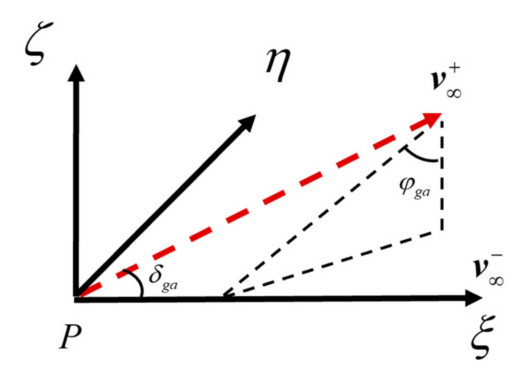
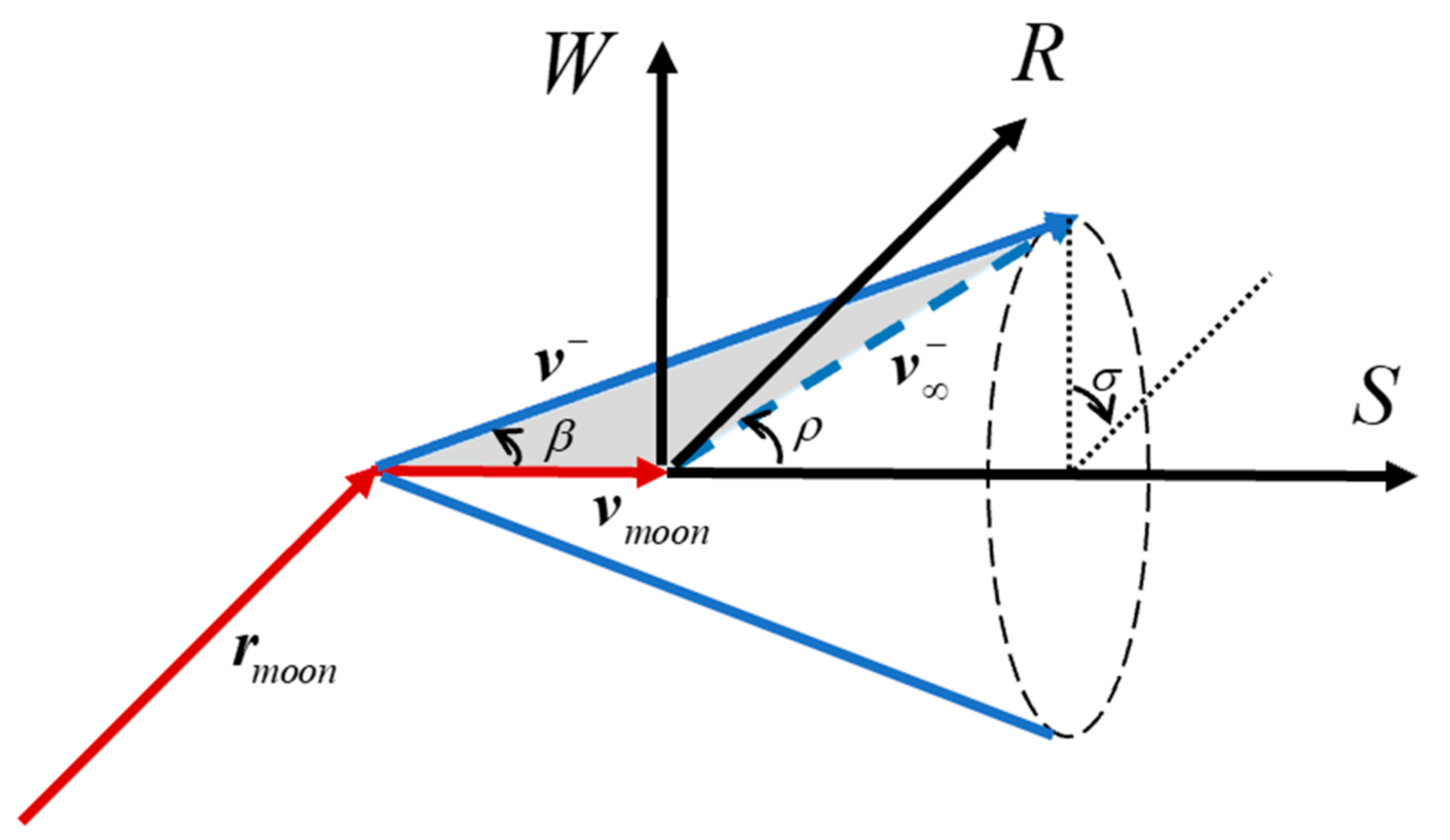
2.2. Gravity Assist Model

The lunar flyby process uses the impulse model. $v_{\infty }^{-}$ and $v_{\infty }^{+}$ indicates pre-flyby and post-flyby moon hyperbolic excessive velocity. The angle between $v_{\infty }^{-}$ and $v_{\infty }^{+}$ is ${\delta }_{ga}$. Generally, the lunar flyby process is described in the coordinate system $P-\xi \eta \zeta$ [24], as shown in Figure 1. $P$ indicates the lunar barycenter. Axis $\xi$ is along the direction of $v_{\infty }^{-}$. Axis $\zeta$ is perpendicular to the plane formed by the pre-flyby geocentric velocity and lunar velocity. $\eta$, $\xi$ and $\zeta$ constitute the right-hand coordinate system. The corresponding three axis unit vectors are $i$, $j$, $k$; the process of lunar flyby can be described as Equation (3).

$$\left\{\begin{array}{l}\delta =2\arcsin \frac{{\mu }_{moon}}{{\mu }_{moon}+\left(R_{moon}+h_{ga}\right)v_{\infty }^2}\\ i=\frac{v_{\infty }^{-}}{‖v_{\infty }^{-}‖},k=\frac{v^{-}\times v_{moon}}{‖v^{-}\times v_{moon}‖},j=k\times i\\ v_{\infty }^{-}=v_{\infty }i\\ v_{\infty }^{+}=v_{\infty }\left[\left(\sin {\delta }_{ga}\cos {\phi }_{ga}\right)k+\left(\sin {\delta }_{ga}\sin {\phi }_{ga}\right)j+\left(\cos {\delta }_{ga}\right)i\right]\end{array}\right.$$

(3)

where ${\mu }_{moon}$ indicates the lunar gravitational constant, $R_{moon}$ indicates the lunar radius, $h_{ga}$ indicates the height of the flyby (the minimal flyby height is 100 km), $v_{moon}$ indicates the lunar velocity, $v^{-}$ indicates the geocentric velocity before the lunar flyby, ${\phi }_{ga}$ indicates the angle between the projection of $v_{\infty }^{+}$ on the $jk$ plane and the axis $k$.

2.3. Earth Aerobraking Model

For the Earth aerobraking model, a simplified model, described in Reference [18], is used in this paper. With a high relative velocity with respect to the Earth, a captured asteroid will pass through the Earth’s atmosphere quickly and, therefore, would remain in the atmosphere for only a short duration. The effect of aerobraking is approximately equivalent to a deceleration impulsive applied at the perigee [18]. The impulsive $\Delta v_{aero}$ generated by aerobraking can be written as [25]:

$$\Delta v_{aero}=\left(1-e^{B{\rho }_{gas}\sqrt{2\pi r_p{H}_S\left(e+1\right)/e}}\right)v_p^{-}$$

(4)

where $B=C_{d}A/\left(2M\right)$; in this model, it is assumed that the density of the atmosphere deceases exponentially from the Earth’s surface, ${\rho }_{gas}={\rho }_0{e}^{-h/H_S}$, ${\rho }_0$ =1.225 kg/m³, and $H_S$ = 7.249 km is the atmospheric scale height [22]; $r_p$ indicates the perigee distance; $v_p^{-}$ indicates geocentric velocity at perigee before aerobraking, $C_d$ indicates the asteroid drag coefficient, assumed as a sphere as 0.47 [20]; $A/M$ is the asteroid area-to-mass ratio. The aerobraking maneuver will lead to mass loss from the asteroid due to the thermal ablation. The mass loss ratio $f$ is defined by [26]

$$f=\frac{m^{-}-m^{+}}{m^{-}}=1-e^{\sigma \left({\left(v_p^{+}\right)}^2-{\left(v_p^{-}\right)}^2\right)/2}$$

(5)

where $v_p^{+}=v_p^{-}+\Delta v_{aero}$ indicates geocentric velocity at perigee after aerobraking. $m^{-}$ and $m^{+}$ indicates the mass of the asteroid before and after aerobraking. $\sigma$ indicates an ablation parameter, assumed to be 2.1 × 10⁻⁸ ${\mathrm{s}}^2/{\mathrm{m}}^2$. After the deceleration of aerobraking, to avoid heading into the atmosphere at the next perigee, a $\Delta v_{raise}$ should be applied at apogee to raise the height of the perigee. The magnitude of $\Delta v_{raise}$ applied at apogee can be written as

$$\Delta v_{raise}=\frac{h_a}{r_a}-\frac{\sqrt{r_a{\mu }_E\left(1-e_n\right)}}{r_a}$$

(6)

where $h_a$ is the magnitude of an asteroid’s angular momentum before aerobraking, $e^{+}$ is the eccentricity of post-aerobraking orbit, $e_n$ is the eccentricity of the orbit with the raised perigee, and $r_{np}$ is the ultimate perigee.

$$h_a=r_p{v}_p^{+},e^{+}=\frac{h_a^2}{r_p{\mu }_E}-1,r_a=\frac{h_a^2}{{\mu }_E\left(1-e^{+}\right)},e_n=\frac{r_a-r_{np}}{r_a+r_{np}}$$

(7)

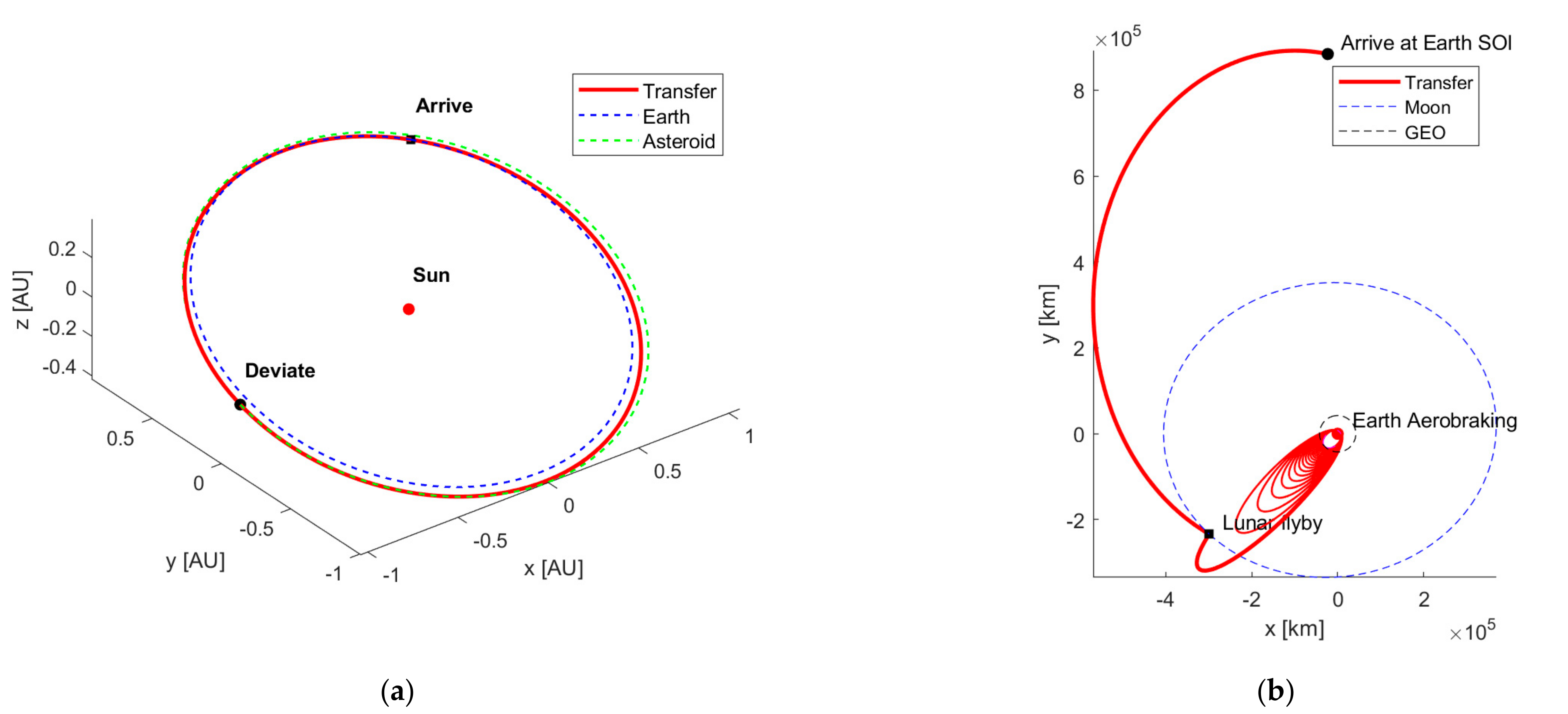
3. Trajectory Design and Optimization

The schematic diagram of lunar flyby plus Earth aerobraking is shown in Figure 2. The inbound fuel consumption is always much larger than the outbound fuel consumption because the spacecraft’s system has more mass after capturing an asteroid [15]. Hence, this work only focuses on the inbound trajectories. The aim is to capture an asteroid in a low-energy and low-inclination orbit, such as GTO. After the asteroid enters the Earth’s Sphere of Influence (SOI), it first uses lunar flyby, then multi-pass aerobraking, for further deceleration. After the multi-pass aerobraking, an impulsive maneuver $\Delta v_{raise}$ is applied at apogee to raise the next perigee to above the atmospheric boundary.

The following sections will introduce the modeling process of three different asteroid capture strategies, including the use of direct capture strategy (just applying decelerating maneuvers without lunar flyby and Earth aerobraking), Earth aerobraking capture strategy and lunar flyby plus Earth aerobraking capture strategy.

3.1. Direct Capture Strategy

The NEA begins to deviate from its original orbit at $t_0$, arriving at Earth’s SOI after $\Delta t_1$ days, and arriving at the perigee after $\Delta t_2$ days. ${\alpha }_{soi}$ and ${\beta }_{soi}$ determine the position vector on the SOI of the Earth. ${\alpha }_p$, ${\beta }_p$ and the height of perigee $h_p$ determine the position vector of perigee. By solving Lambert’s problem for the heliocentric arc, the impulse $\Delta v_0$ executed at $t_0$ can be calculated. By solving Lambert’s problem for the geocentric arc, the impulse $\Delta v_{soi}$ executed at $\left(t_0+\Delta t_1\right)$ can be calculated. A deceleration maneuver $\Delta v_f$ is performed at the perigee to directly capture the asteroid in the target orbit. The total velocity change $\Delta v_{total}$ is

$$\Delta v_{total}=‖\Delta v_0‖+‖\Delta v_{soi}‖+‖\Delta v_f‖$$

(8)

The decision variables are

$$x=\left[t_0,\Delta t_1,\Delta t_2,{\alpha }_{soi},{\beta }_{soi},{\alpha }_p,{\beta }_p\right]$$

(9)

the objective function is

$$J=10\Delta v_{total}+M_p+i_p$$

(10)

where $M_p$ and $i_p$ indicate the mean anomaly and the inclination at $\left(t_0+\Delta t_1+\Delta t_2\right)$, which is used to make sure that the Earth aerobraking is performed at the perigee. The constraints are summarized in the

Table 1. Constraints of the direct capture strategy.

Constraints	Value
Target orbit	GTO (200 km × 36,000 km)
Deviate date	01/01/2030–01/01/2050

.

3.2. Earth Aerobraking Capture Strategy

The NEA begins to deviate from its original orbit at $t_0$, arriving at Earth’s SOI after $\Delta t_1$ days and arriving at Earth’s atmosphere after $\Delta t_2$ days. ${\alpha }_{soi}$ and ${\beta }_{soi}$ indicates the location angles on the SOI of the Earth. ${\alpha }_{aero}$, ${\beta }_{aero}$ and the height of aerobraking $h_{aero}$ determine the position of the vector Earth aerobraking. By solving Lambert’s problem in the heliocentric arc, the impulse $\Delta v_0$, executed at $t_0$, can be calculated. By solving Lambert’s problem in the geocentric arc, the impulse $\Delta v_{soi}$, executed at $\left(t_0+\Delta t_1\right)$, can be calculated. By providing the aerobraking height $h_{aero}$, the relative velocity of the asteroid at perigee, with respect to the Earth before aerobraking ($v_p^{-}$) and after aerobraking ($v_p^{+}$), can be determined using the Earth aerobraking model. If the orbital energy of the asteroid relative to the Earth is greater than zero after the first Earth aerobraking (if the orbital energy is less than zero, there will be no possibility of further deceleration by Earth aerobraking), the magnitude of $\Delta v_p$ is obtained by the following equation

$$‖\Delta v_p‖=‖v_p^{+}‖-\sqrt{2\frac{{\mu }_E}{‖r_p‖}}$$

(11)

where $r_p$ is the position vector of the Earth aerobraking, ${\mu }_E$ is the gravitational constant of the Earth. Multi-pass Earth aerobraking can be further considered to achieve a sufficiently low energy orbit. The mass loss ratio $f_i$ of each deceleration can be calculated by the Earth aerobraking model, with the total mass loss ratio $f_{total}$ of n-times Earth aerobraking described as follows

$$\left\{\begin{array}{c}{m}^{+}=m^{-}{\displaystyle \prod _{i=1}^n\left(1-f_i\right)}\\ f_{total}=\frac{m^{-}-m^{+}}{m^{-}}\end{array}\right.$$

(12)

After the decelerations of Earth aerobraking, to avoid heading into the atmosphere at the next perigee, the impulse $\Delta v_{raise}$ should be executed at the apogee to raise the height of perigee. The total velocity change $\Delta v_{total}$ is

$$\Delta v_{total}=‖\Delta v_0‖+‖\Delta v_{soi}‖+‖\Delta v_p‖+‖\Delta v_{raise}‖$$

(13)

The decision variables are

$$x=\left[t_0,\Delta t_1,\Delta t_2,{\alpha }_{soi},{\beta }_{soi},{\alpha }_{aero},{\beta }_{aero}\right]$$

(14)

the objective function is

$$J=10\Delta v_{total}+f_{total}+M_p+i_p$$

(15)

where $M_p$ and $i_p$ indicate the mean anomaly and the inclination at Earth aerobraking, which is used to make sure that the Earth aerobraking is performed at the perigee. The constraints are summarized in the

Table 2. Constraints of the Earth aerobraking capture strategy.

Constraints	Value
Target orbit	GTO (200 km × 36,000 km)
Deviate date	01/01/2030–01/01/2050
Height of aerobraking	≥60 km

.

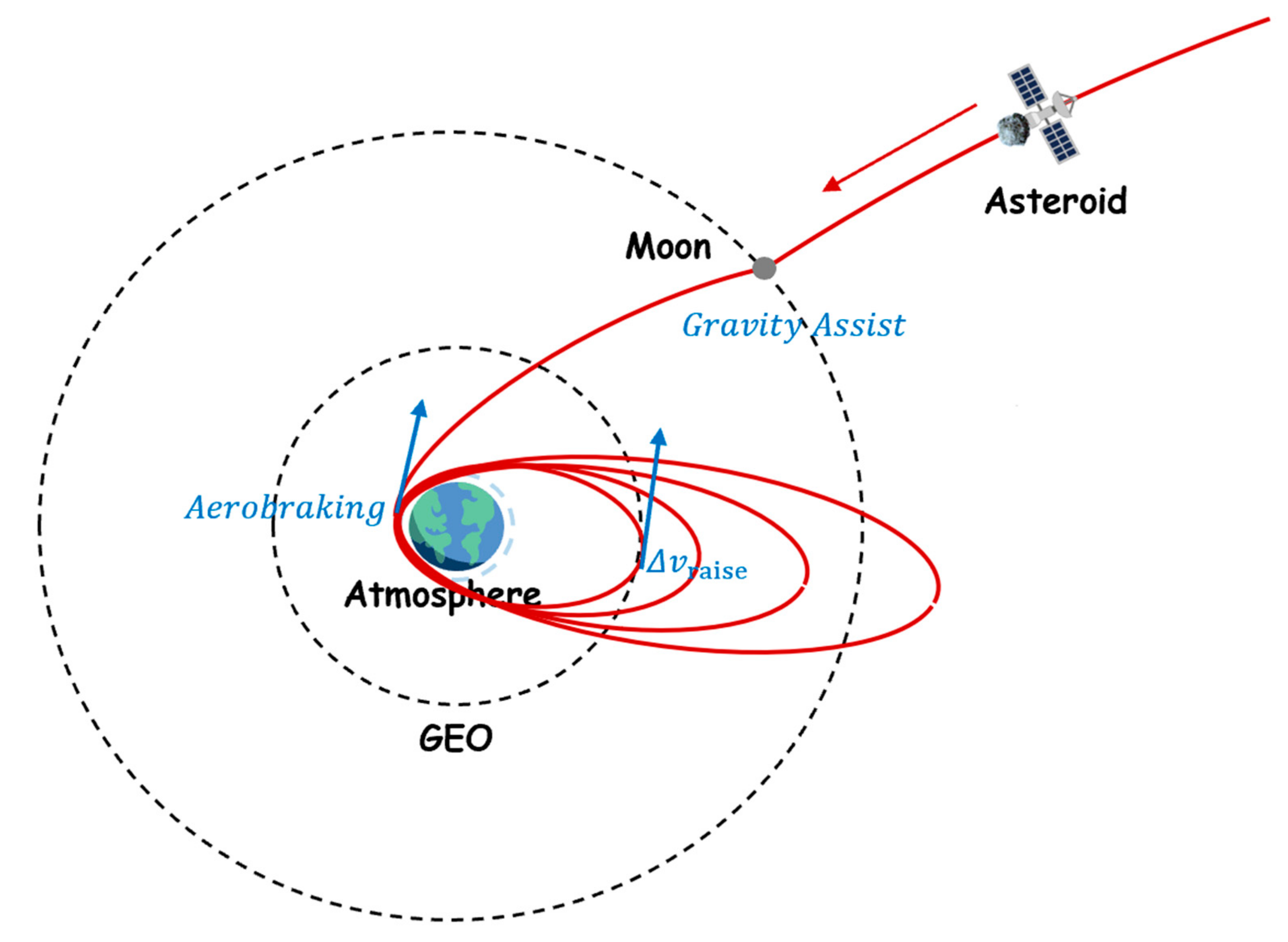
3.3. Lunar Flyby plus Earth Aerobraking Capture Strategy

The NEA begins to deviate from its original orbit at $t_0$, arriving at Earth’s SOI after $\Delta t_1$ days, arriving at the Moon after $\Delta t_2$ days, and arriving at the perigee after $\Delta t_3$. ${\alpha }_{soi}$ and ${\beta }_{soi}$ indicates the location angles on the SOI of the Earth. $h_{ga}$ and ${\phi }_{ga}$ indicate flyby height and angle parameter. ${\alpha }_{aero}$, ${\beta }_{aero}$ and $h_{aero}$ determines the location of Earth aerobraking. By solving Lambert’s problem in the heliocentric arc, impulse $\Delta v_0$ executed at $t_0$ can be calculated. By solving Lambert’s problems in the geocentric arcs, the impulse $\Delta v_{soi}$, executed at $\left(t_0+\Delta t_1\right)$, and the impulse $\Delta v_{aftga}$, executed at $\left(t_0+\Delta t_1+\Delta t_2\right)$, can be calculated. By providing the height of aerobraking $h_{aero}$, the relative velocity of the asteroid at perigee with respect to the Earth before aerobraking ($v_p^{-}$) and after aerobraking ($v_p^{+}$) can be determined by the Earth aerobraking model. The impulse $\Delta v_p$ at perigee is executed if the orbital energy of the asteroid relative to the Earth is greater than zero after the first Earth aerobraking, which can be calculated by Equation (11). Multi-pass Earth aerobraking can further be considered to achieve a sufficiently low energy orbit. The total mass loss ratio $f_{total}$ of n-times Earth aerobraking can be calculated by Equation (12). Furthermore, the impulse $\Delta v_{raise}$ at apogee is executed to raise the perigee radius. The total velocity change $\Delta v_{total}$ is

$$\Delta v_{total}=‖\Delta v_0‖+‖\Delta v_{soi}‖+‖\Delta v_{aftga}‖+‖\Delta v_p‖+‖\Delta v_{raise}‖$$

(16)

The decision variables are

$$x=\left[t_0,\Delta t_1,\Delta t_2,\Delta t_3,{\alpha }_{soi},{\beta }_{soi},h_{ga},{\phi }_{ga},{\alpha }_{aero},{\beta }_{aero}\right]$$

(17)

the objective function is

$$J=10\Delta v_{total}+f_{total}+M_p+i_p$$

(18)

the constraints are summarized in the

Table 3. Constraints of the lunar flyby plus Earth aerobraking capture strategy.

Constraints	Value
Target orbit	GTO (200 km × 36,000 km)
Deviate date	01/01/2030–01/01/2050
Height of aerobraking	≥60 km
Height of lunar flyby	≥100 km

.

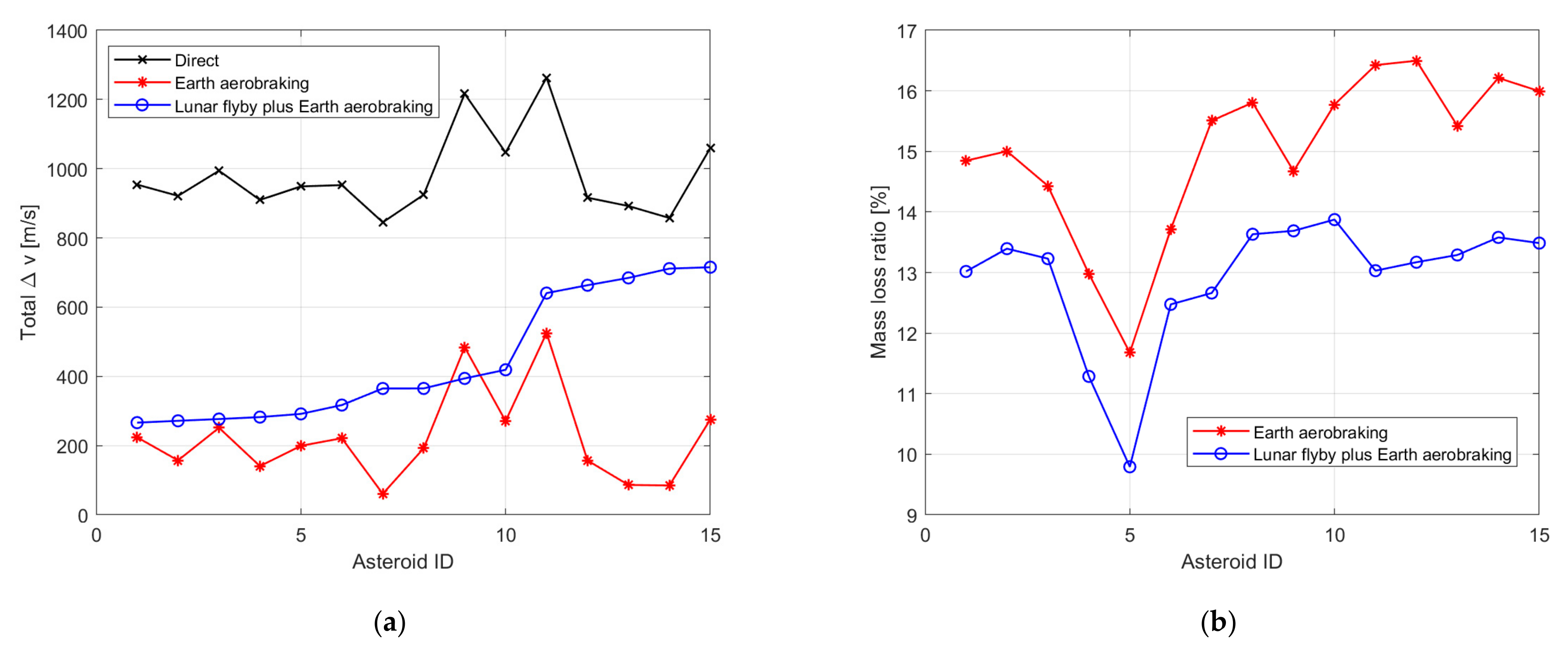
4. Simulation Results

To ensure that the captured asteroids do not pose a threat to the earth, only small asteroids with a diameter of less than 30 m (calculated by absolute magnitude downloaded from JPL Small-body Database), which can be disintegrated by the Earth’s atmosphere [27,28], are considered in this paper. The diameter of an asteroid can be estimated from the albedo and magnitude [29], assuming that the asteroid albedo is 0.154 and the asteroid density is 2.6 g/cm³ [18]. Using GTO as the target captured orbit, by using lunar flyby plus Earth aerobraking capture strategy, 15 asteroids with the lowest total velocity change ($\Delta v_{total}$) are shown in

Table 4. Otimization results of using lunar flyby plus Earth aerobraking strategy.

Asteroid ID	Name	Diameter (m)	Dv at Deviation ${\Delta }{\mathit{v}}_0$ (m/s)	Dv at Earth SOI ${\Delta }{\mathit{v}}_{\mathit{s}\mathit{o}\mathit{i}}$ (m/s)	Dv after Flyby ${\Delta }{\mathit{v}}_{\mathit{a}\mathit{f}\mathit{t}\mathit{g}\mathit{a}}$ (m/s)	Dv at Perigee ${\Delta }{\mathit{v}}_{\mathit{p}}$ (m/s)	Dv at Apogee ${\Delta }{\mathit{v}}_{\mathit{r}\mathit{a}\mathit{i}\mathit{s}\mathit{e}}$ (m/s)	${\Delta }{\mathit{v}}_{\mathit{t}\mathit{o}\mathit{t}\mathit{a}\mathit{l}}$ (m/s)	${\mathit{f}}_{\mathit{t}\mathit{o}\mathit{t}\mathit{a}\mathit{l}}$ (%)	Aerobraking Times	Deviate Date	Capture Date
1	2007 UN12	6.16	214.83	28.75	7.99	0.00	14.73	266.30	13.02	12	25/10/2032	23/09/2034
2	2008 EA9	9.77	181.87	54.82	20.16	0.00	14.74	271.59	13.39	19	13/09/2048	09/01/2049
3	2010 UE51	7.41	195.85	58.55	7.57	0.00	14.75	276.72	13.23	14	31/08/2035	13/12/2036
4	2021 GM1	2.77	202.67	43.70	21.13	0.00	14.81	282.31	11.28	5	30/12/2034	22/06/2036
5	2020 CD3	1.55	177.32	85.93	13.50	0.00	14.78	291.54	9.79	3	10/10/2043	30/06/2045
6	2006 RH120	4.26	163.72	117.72	20.81	0.00	14.81	317.06	12.47	8	27/02/2049	14/11/2049
7	2019 XV	4.90	209.21	130.75	10.30	0.00	14.78	365.05	12.66	9	22/10/2033	23/10/2034
8	2021 GK1	12.82	268.27	64.34	17.83	0.00	14.71	365.15	13.63	25	15/12/2046	05/06/2047
9	2012 TF79	11.27	353.69	24.67	1.01	0.00	14.69	394.06	13.69	23	25/02/2040	16/11/2041
10	2016 TB57	20.41	264.18	75.85	64.28	0.00	14.71	419.03	13.87	42	29/12/2036	07/12/2038
11	2015 VO142	5.62	553.08	60.46	12.29	0.00	14.76	640.59	13.03	11	08/03/2043	01/01/2045
12	2019 NX5	5.13	369.65	264.95	13.93	0.00	14.79	663.33	13.17	11	29/12/2046	09/07/2048
13	2010 VQ98	7.76	362.42	292.02	15.42	0.00	14.67	684.52	13.29	16	11/11/2038	04/11/2039
14	2011 MD	8.51	65.08	39.23	592.30	0.00	14.70	711.32	13.58	18	03/03/2048	18/06/2049
15	2010 JW34	8.12	550.31	29.63	120.69	0.00	14.71	715.34	13.49	17	18/06/2044	08/04/2046

. Based on these 15 asteroids’ information, the optimization results of the Earth aerobraking capture strategy and direct capture strategy are shown in

Table 5. Optimization results of Earth aerobraking capture strategy.

Name	Diameter (m)	Dv at Deviation ${\Delta }{\mathit{v}}_0$ (m/s)	Dv at Earth SOI ${\Delta }{\mathit{v}}_{\mathit{s}\mathit{o}\mathit{i}}$ (m/s)	Dv at Perigee ${\Delta }{\mathit{v}}_{\mathit{p}}$ (m/s)	Dv at Apogee ${\Delta }{\mathit{v}}_{\mathit{r}\mathit{a}\mathit{i}\mathit{s}\mathit{e}}$ (m/s)	${\Delta }{\mathit{v}}_{\mathit{t}\mathit{o}\mathit{t}\mathit{a}\mathit{l}}$ (m/s)	${\mathit{f}}_{\mathit{t}\mathit{o}\mathit{t}\mathit{a}\mathit{l}}(\%)$	Aerobraking Times	Deviate Date	Capture Date
2019 XV	4.90	44.97	0.95	0.00	14.77	60.70	15.51	11	13/08/2031	02/11/2034
2011 MD	8.51	39.78	9.06	20.87	15.18	84.89	16.21	19	29/06/2046	16/06/2049
2010 VQ98	7.76	69.00	2.62	0.00	14.66	86.28	15.42	20	26/01/2039	28/10/2040
2021 GM1	2.77	106.96	19.02	0.00	14.71	140.68	12.98	6	07/01/2033	21/04/2035
2019 NX5	5.13	83.61	13.87	44.11	15.44	157.03	16.50	12	13/01/2047	27/07/2048
2008 EA9	9.77	139.84	2.71	0.00	14.68	157.23	15.00	23	25/01/2031	14/01/2034
2021 GK1	12.82	163.01	12.65	1.89	14.78	192.33	15.81	28	14/07/2045	07/06/2047
2020 CD3	1.55	183.17	1.66	0.00	14.57	199.40	11.68	4	26/09/2043	16/05/2045
2006 RH120	4.26	147.91	58.63	0.00	14.73	221.27	13.72	9	21/03/2049	14/10/2049
2007 UN12	6.16	207.28	1.94	0.00	14.73	223.95	14.85	14	12/02/2032	27/08/2034
2010 UE51	7.41	236.63	0.14	0.00	14.75	251.52	14.43	15	24/12/2048	29/10/2049
2016 TB57	20.41	215.12	3.05	37.82	14.77	270.76	15.77	43	31/05/2037	24/11/2038
2010 JW34	8.12	242.08	7.46	11.06	14.97	275.57	15.99	18	17/08/2043	25/04/2045
2012 TF79	11.27	458.92	10.62	0.00	14.58	484.12	14.67	28	31/01/2040	14/10/2042
2015 VO142	5.62	397.31	21.54	90.91	15.37	525.13	16.42	13	17/01/2033	01/03/2035

and

Table 6. Optimization results of direct capture strategy.

Name	Diameter (m)	Dv at Deviation ${\Delta }{\mathit{v}}_0$ (m/s)	Dv at Earth SOI ${\Delta }{\mathit{v}}_{\mathit{s}\mathit{o}\mathit{i}}$ (m/s)	Dv at Perigee ${\Delta }{\mathit{v}}_{\mathit{p}}$ (m/s)	${\Delta }{\mathit{v}}_{\mathit{t}\mathit{o}\mathit{t}\mathit{a}\mathit{l}}$ (m/s)	Deviate Date	Capture Date
2010 VQ98	7.76	72.02	0.80	772.33	845.15	10/07/2038	25/10/2040
2021 GM1	2.77	107.99	5.36	744.19	857.55	14/01/2032	16/04/2034
2011 MD	8.51	61.35	2.66	828.10	892.10	20/05/2047	15/06/2049
2021 GK1	12.82	104.58	5.88	799.23	909.68	29/08/2046	09/06/2047
2006 RH120	4.26	167.48	3.40	745.35	916.23	17/03/2049	28/10/2049
2019 XV	4.90	98.82	17.86	804.80	921.48	19/07/2046	08/10/2049
2010 UE51	7.41	165.19	4.50	755.02	924.70	30/12/2046	01/11/2049
2020 CD3	1.55	148.12	67.45	733.20	948.77	18/12/2042	14/05/2045
2010 JW34	8.12	123.79	23.51	805.32	952.62	25/02/2042	02/05/2044
2008 EA9	9.77	173.24	11.33	769.44	954.01	01/01/2031	20/12/2033
2007 UN12	6.16	225.68	6.58	761.82	994.08	07/11/2032	06/09/2034
2019 NX5	5.13	179.06	14.17	853.51	1046.73	20/11/2046	13/06/2048
2016 TB57	20.41	225.05	4.20	830.62	1059.87	26/01/2038	13/12/2038
2015 VO142	5.62	401.47	3.18	811.86	1216.50	24/02/2033	31/01/2035
2012 TF79	11.27	527.87	0.72	734.42	1263.01	04/03/2040	06/11/2041

. The lowest $\Delta v_{total}$ of lunar flyby plus Earth aerobraking capture strategy is 266.3 m/s (asteroid 2007 UN12), the lowest $\Delta v_{total}$ of Earth aerobraking capture strategy is 60.70 m/s (asteroid 2019 XV), while the lowest $\Delta v_{total}$ of direct capture strategy is 772.33 m/s (asteroid 2010 VQ98).

Numbing the asteroids according to the order of in Table 4, Figure 3 compares the effects of three different capture strategies on 15 asteroids from the perspectives of the total velocity change $\Delta v_{total}$ and the total mass loss ratio $f_{total}$.

By comparing the direct capture strategy with the Earth aerobraking strategy, the Earth aerobraking capture strategy shows a significant advantage over the direct capture strategy in terms of total velocity change $\Delta v_{total}$. It is clear from the Figure 3a that the red line and the black line show a consistent trend. This is because the $\Delta v$ in heliocentric arc of the Earth aerobraking capture strategy and the direct capture strategy are similar, the main difference is that the Earth aerobraking capture strategy can save the deceleration maneuver $\Delta v_f$ at the perigee. For the direct capture strategy, asteroid 2012 TF79 requires the highest $\Delta v_{total}$, which is 1263.01 m/s. If the Earth aerobraking capture strategy is used, the $\Delta v_{total}$ of asteroid 2012 TF79 can be reduced to 484.12 m/s, with a 14.67% of mass loss ratio, due to the thermal ablation. This comparison results demonstrate the high efficiency of using Earth aerobraking when the target orbit is low-energy.

By comparing the lunar flyby plus Earth aerobraking with the Earth aerobraking capture strategy, the most significant advantage of the lunar flyby plus Earth aerobraking capture strategy is that it can reduce the total mass loss ratio $f_{total}$, as this can be reduced by about 0.98–3.39%. For example, for an asteroid with a diameter of 5 m, the mass is about 170 tons (with a density of 2.6 g/cm³), reducing the mass loss ratio by 1% means that 1701.7 kg of the asteroid materials can be saved. For the asteroid 2012 TF79, the lunar flyby plus Earth aerobraking capture strategy can also reduce the total velocity change $\Delta v_{total}$ (from 484.12 m/s to 394.06 m/s). For asteroid 2007 UN12 and 2010 UE51, the $\Delta v_{total}$ required for the lunar flyby plus Earth aerobraking and the Earth aerobraking capture strategy are similar. For most asteroids, although the reduction in total mass loss ratio $f_{total}$ leads to an increase in total velocity change $\Delta v_{total}$, this is a trade-off problem that requires further comprehensive analysis by decision makers.

Taking asteroid 2012 TF79 (with a diameter of 11.27 m) as an example,

Table 7. Comparison details of total velocity change and total mass loss ratio.

Name	Diameter (m)	Mass (tons)	Total Velocity Change ${\Delta }{\mathit{v}}_{\mathit{t}\mathit{o}\mathit{t}\mathit{a}\mathit{l}}$			Total Mass Loss Ratio ${\mathit{f}}_{\mathit{t}\mathit{o}\mathit{t}\mathit{a}\mathit{l}}$
			Aerobraking (m/s)	Lunar Flyby plus Aerobraking (m/s)	Fuel Saved (tons)	Aerobraking (%)	Lunar Flyby plus Aerobraking (%)	Mass Saved (tons)
2012 TF79	11.27	1946.55	484.12	394.06	5.87	14.67	13.69	19.17

gives the details of a comparison between the Earth aerobraking capture strategy and lunar flyby plus aerobraking capture strategy from the perspectives of total velocity change $\Delta v_{total}$ and total mass loss ratio $f_{total}$. Compared with the Earth aerobraking capture strategy, by using the lunar flyby plus Earth aerobraking capture strategy, 5.87 tons of fuel can be saved, while 19.17 tons of asteroid materials can be saved due to the alleviation of thermal ablation. Figure 4 shows the corresponding heliocentric and geocentric transfer trajectories. More fuel and material mass can be saved as the size of the asteroid increases.

5. Discussion

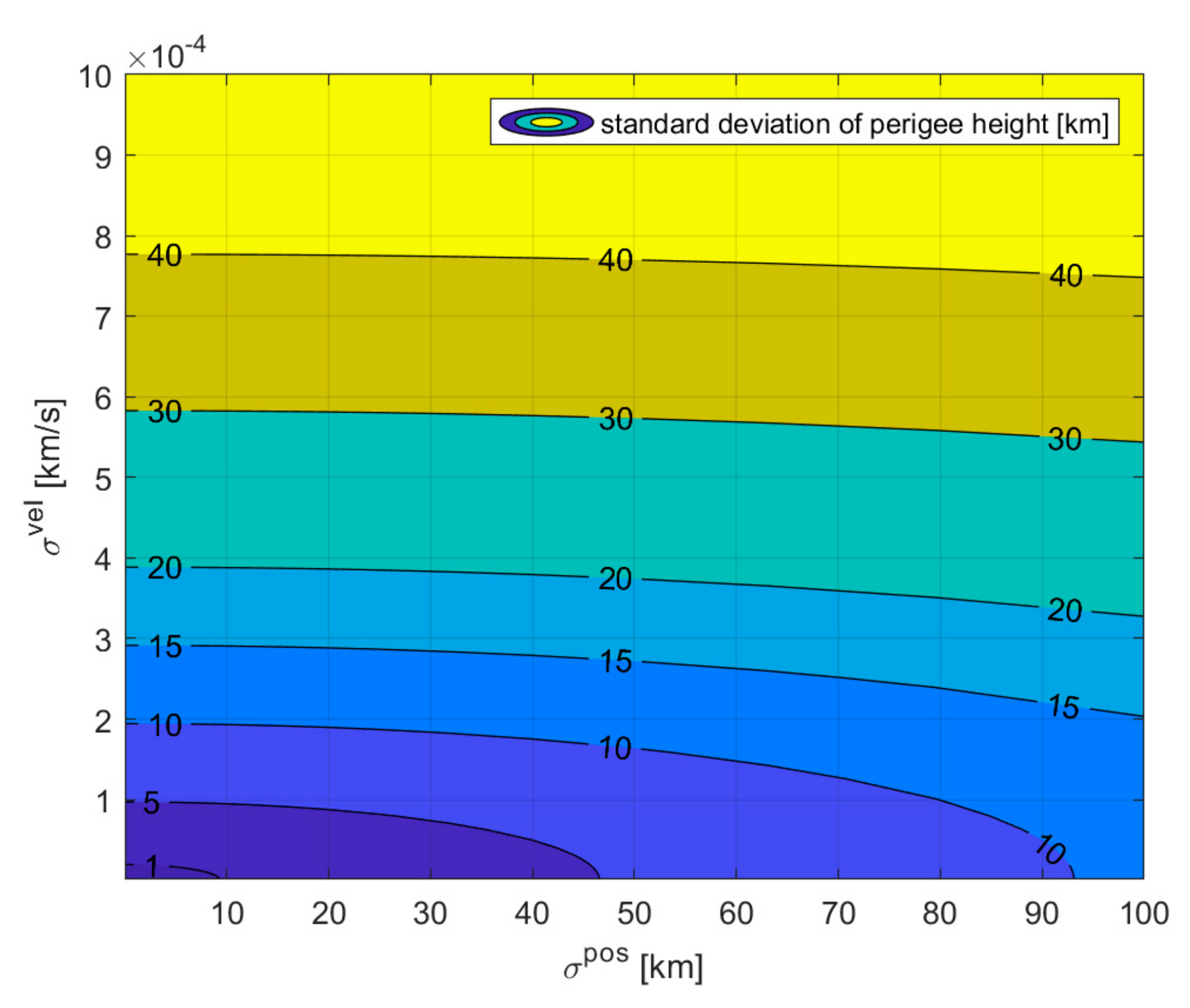
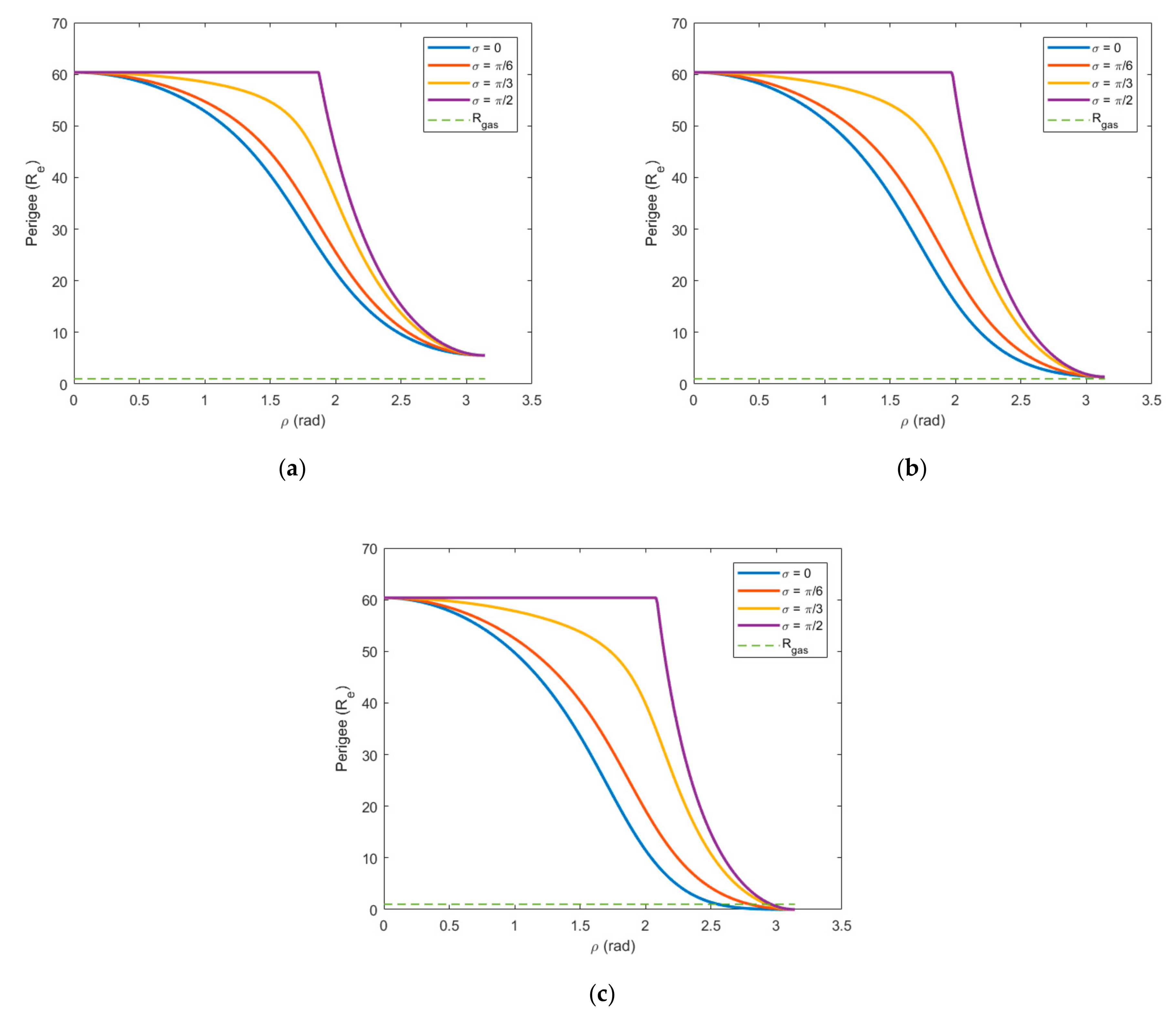
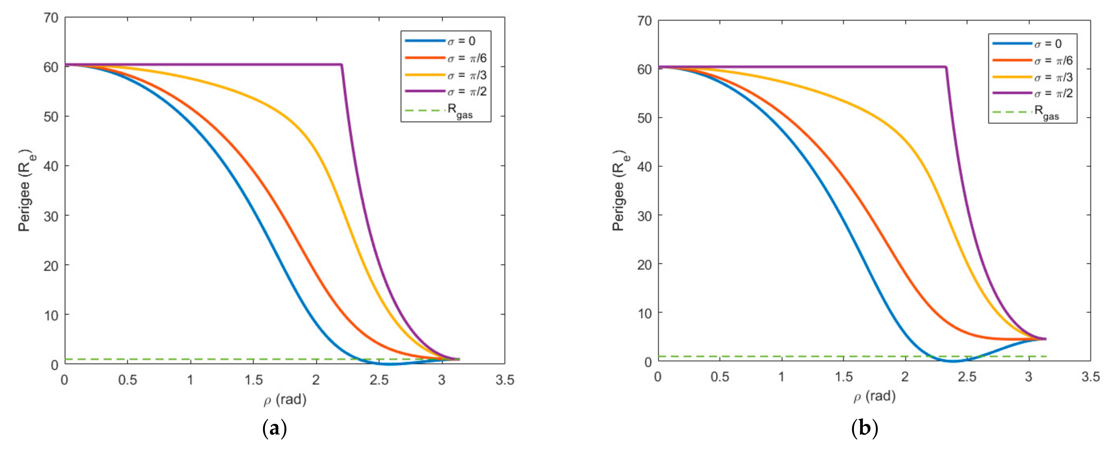
5.1. Sensitivity of Using Lunar Flyby plus Earth Aerobraking

If the flyby targeting goes wrong, the asteroid will be injected into an aerobraking trajectory with a lower or higher perigee. This section discusses the sensitivity of the aerobraking perigee to the entry conditions at the Moon; that is, the influence of pre-flyby position and velocity errors on the post-flyby perigee height is studied.

Post-flyby position ${\tilde{r}}_{aftga}$ and velocity ${\tilde{v}}_{aftga}$, which including the uncertainties, can be described as follows

$$\begin{array}{l}{\tilde{r}}_{aftga}=\left[\begin{array}{c}{r}_{bfga\_x}+{\sigma }_x^{pos}randn\left(0,1\right)\\ r_{bfga\_y}+{\sigma }_y^{pos}randn\left(0,1\right)\\ r_{bfga\_z}+{\sigma }_z^{pos}randn\left(0,1\right)\end{array}\right]\\ {\tilde{v}}_{aftga}=\left[\begin{array}{c}{v}_{bfga\_x}+{\sigma }_x^{vel}randn\left(0,1\right)\\ v_{bfga\_y}+{\sigma }_y^{vel}randn\left(0,1\right)\\ v_{bfga\_z}+{\sigma }_z^{vel}randn\left(0,1\right)\end{array}\right]+\Delta v_{ga}\\ \Delta v_{ga}=v_{\infty }^{+}-v_{\infty }^{-}\end{array}$$

(19)

$r_{bfga}$ and $v_{bfga}$ indicates the pre-flyby position and velocity, while ${\tilde{r}}_{aftga}$ and ${\tilde{v}}_{aftga}$ indicates the post-flyby position and velocity involving the uncertainties. randn(0,1) is a Gaussian random number generator with zero mean and a unit standard deviation, ${\sigma }^{pos}$ and ${\sigma }^{vel}$ indicates the expected pre-flyby position (indicated by superscript pos) and velocity (indicated by superscript vel) uncertainties. $\Delta v_{ga}$ indicates the velocity change caused by lunar flyby, while $v_{\infty }^{-}$ and $v_{\infty }^{+}$ indicates pre-flyby and post-flyby hyperbolic excessive velocity, which are described in Section 2.2. Furthermore, the corresponding perigee distance can be calculated by using the calculation method described in Section 3.3.

Taking asteroid 2012 TF79’s optimization results as the example,

Table 8. Asteroid 2012 TF79’s pre-flyby state and associated $\sigma$ values.

	Nom Value	$\mathit{\sigma }$	Unit
$r_x$	−298802.266580121	${10}^{-1}$	km
$r_y$	−233805.590770561	${10}^{-1}$	km
$r_z$	−105546.565356819	${10}^{-1}$	km
$v_x$	0.855934533216751	${10}^{-5}$	km/s
$v_y$	−0.495537514308965	${10}^{-5}$	km/s
$v_z$	0.642469340439085	${10}^{-5}$	km/s

shows the nominal pre-flyby state and the associated $\sigma$ of the asteroid 2012 TF79, while

Table 9. Asteroid 2012 TF79’s deterministic information.

	Description	Unit
Julian Date of flyby	2466872.98992665	JD
Coordinate reference frame	International Celestial Reference Frame (ICRF)
$\mathrm{Flyby}\mathrm{height}{h}_{ga}$	380.966926993433	km
$\mathrm{Flyby}\mathrm{angle}{\phi }_{ga}$	4.18119720291364	rad
$\mathrm{Dv}\mathrm{after}\mathrm{flyby}\Delta v_{aftga}$	(−0.000282473846928810; −0.000943184415699683; 0.000208519543117069)	km/s

shows the deterministic information of the asteroid 2012 TF79.

The propagation of uncertainties is performed by Monto Carlo method. More specifically, 10,000 virtual pre-flyby states are generated with a Gaussian distribution with mean value and standard deviation as in Table 8. According to the simulation results, if the order of magnitude of ${\sigma }^{pos}$ is ${10}^{-1}$ km and of ${\sigma }^{vel}$ is ${10}^{-5}$ km/s, the standard deviation of the perigee height is 0.51 km.

Furthermore, the impacts of different ${\sigma }^{pos}$ and ${\sigma }^{vel}$ on the perigee height are discussed. Monte Carlo method provides true trajectory statistics, but it is computationally intensive [30,31]. The Unscented Transform (UT), a method to calculate the mean value and the covariance of a probability distribution of a random variable that undergoes a nonlinear transformation [32] is introduced to improve the calculation efficiency. Considering ${\sigma }^{pos}\in [0,{10}^2]$ km and ${\sigma }^{vel}\in [0,{10}^{-3}]$ km/s, Figure 5 shows the impacts of different ${\sigma }^{pos}$ and ${\sigma }^{vel}$ on the perigee height standard deviation. According to simulation results, if the order of magnitude of ${\sigma }^{pos}$ and ${\sigma }^{vel}$ can be lower than ${10}^{-1}$ km and ${10}^{-5}$ km/s respectively, the standard deviation of perigee height can be controlled within about 1 km.

5.2. The Conditions of Using Lunar Flyby plus Earth Aerobraking without Maneuvers

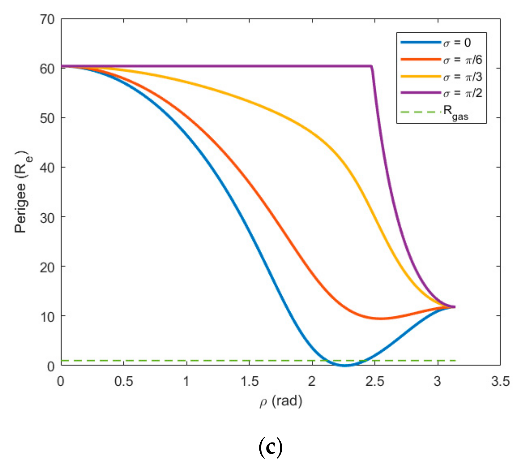
It can be seen from Table 4 that, compared with other asteroids, asteroid 2012 TF79 has a very small maneuver $d{v}_{aftga}$ between lunar flyby and Earth aerobraking (Only 1.01 m/s). In this section, based on the geometric characteristics of the lunar flyby, we further discuss the conditions that do not require maneuvering between the lunar flyby and Earth aerobraking.

In order to visually describe the process of lunar flyby, we introduce the RSW coordinate system [33]. Taking the end point of tangential velocity as the origin (this paper assumes that lunar orbit eccentricity is zero, so the lunar tangential velocity is equal to the lunar velocity): Lunar tangential direction is the R axis; the normal direction of lunar orbit is the W axis; S, R and W axes satisfy the right-hand orthogonal rule. The direction of $v_{\infty }$ can be described by $\rho$ and $\sigma$ in the RSW coordinate system, where $\rho$ is the angle with the S axis, and $\sigma$ is the angle between the projection of $v_{\infty }$ in the R-W plane and the R axis, which is positive when counter-clockwise around the S axis. $\beta$ indicates the angle between asteroid velocity and lunar velocity. The velocity geometric relationship at lunar flyby is shown in Figure 6. By considering the geometric relationship, the lunar flyby process can be completely equivalent to the geometric problem of rotating $v_{\infty }$. This will make the analysis of lunar flyby process more intuitive.

The inclination between the lunar orbital plane and equatorial plane varies between 4°57′ and 5°19′, with an average of about 5°9′. This paper regards the lunar inclination as the low-inclination. Therefore, the target direction of $v_{\infty }$ should be in the lunar orbit plane, that is, $\sigma =0$ or $\pi$. The geometric characteristics show that when $v_{\infty }$ is in the lunar orbit plane, the angle between $v_{moon}$ and $v_{\infty }$ can also be adjusted by single flyby or multiple lunar flybys. The following is a study of the variation in orbital energy with the $v_{\infty }$ direction in the case of $v_{\infty }$ in the lunar orbit plane.

Regarding the geometric relationship, the orbital energy after lunar flyby is only related to $\rho$, when keeping $\rho$ invariant, different $\sigma$ indicates the post-flyby orbit with a different eccentricity and orientation but the same energy. Therefore, the post-flyby velocity $‖v^{+}‖$ can be expressed as

$$‖v^{+}‖=\sqrt{v_x^2+v_y^2}=\sqrt{{(v_{\infty }\cos \rho +v_{moon})}^2+{(v_{\infty }\sin \rho )}^2}$$

(20)

The partial derivative of $‖v^{+}‖$ is as follows

$$\frac{\partial ‖v^{+}‖}{\partial \rho }=-\frac{\sin \rho v_{moon}}{\sqrt{{(v_{\infty }\cos \rho +v_{moon})}^2+{(v_{\infty }\sin \rho )}^2}}<0$$

(21)

It can be seen from the above equation that keeping $\sigma$ constant and rotating $v_{\infty }$ in the shadow plane (shown in Figure 6) is the most efficient way of changing the orbital energy, due to the derivative of the above formula is always negative. The $v^{+}$ decreases as the $\rho$ increases, and the minimal $‖v^{+}‖$ occurs when $v_{\infty }$ is opposite to $v_{moon}$. When $v_{\infty }$ > $v_{moon}$, the minimal-energy orbit that can be formed is the retrograde orbit; when $v_{\infty }$ < $v_{moon}$, the minimal-energy orbit that can be formed is the prograde orbit.

5.2.1. The Case of v_∞ < v_moon

To consider whether it is possible to further utilize Earth aerobraking after lunar flyby, it is necessary to study the height relationship between the post-flyby perigee and the boundary of the atmosphere. The value of $\rho$ uniquely determines the semi-major axis of the asteroid. The post-flyby eccentricity can be calculated by the following formula

$$e=\sqrt{\frac{r_{moon}{v}_t^2}{{\mu }_E}\left(\frac{r_{moon}}{{\mu }_E}{‖v^{+}‖}^2-2\right)+1}$$

(22)

where $\left\{\begin{array}{c}‖v^{+}‖=\sqrt{v_{moon}^2+v_{\infty }^2+2v_{moon}{v}_{\infty }\cos \rho }\\ v_t=\sqrt{{\left(v_{\infty }\sin \rho \sin \sigma \right)}^2+{\left(v_{moon}+v_{\infty }\cos \rho \right)}^2}\end{array}\right.$.

The semi-major axis can be calculated by the following formula

$$a=\frac{{\mu }_E{r}_{moon}}{2{\mu }_E-r_{moon}{‖v^{+}‖}^2}$$

(23)

Therefore, the post-flyby perigee can be calculated as follows

$$r_p\left(\rho \right)=a\left(1-e\right)$$

(24)

According to Tan, et al. [18], once the height at perigee above the Earth’s surface is larger than a critical value (approximately 100 km), the Earth aerobraking effect can be neglected. Therefore, in this paper, we use the critical height of 100 km to determine whether an Earth aerobraking occurs (the critical distance of atmosphere is denoted by $R_{gas}$ in the following text).

Assuming the mean orbital velocity of Moon is 1.022 km/s, we study three cases of $v_{\infty }$ equal to 0.6 km/s, 0.8 km/s, 1 km/s. The variation in perigee $r_p\left(\rho \right)$ with $\rho$ is simulated by $\sigma$ equal to 0, $\pi /6$, $\pi /3$ and $\pi /2$. The following figures give the simulation results, where the dotted line indicates the critical distance of atmosphere $R_{gas}$.

According to Figure 7, when $v_{\infty }$ < $v_{moon}$, whatever the value of $\sigma$, the minimal perigee distance occurs when the $v_{\infty }$ is opposite the $v_{moon}$ ($\rho =\pi ,\beta =0$). Therefore, the analytical expression of the minimal perigee distance can be calculated as follows:

$$r_{p\min }=\frac{r_{moon}^2{\left(v_{moon}-v_{\infty }\right)}^2}{2{\mu }_E-r_{moon}{\left(v_{moon}-v_{\infty }\right)}^2}$$

(25)

As $v_{\infty }$ increases, the minimum of the perigee height distance will gradually decrease until it is below the $R_{gas}$. When the minimal perigee distance is equal to the $R_{gas}$, a critical value $v_{\infty (c)}$ (about 0.83 km/s ) can be found, as follows,

$$v_{\infty (c)}=v_{moon}-\sqrt{2{\mu }_E\left(\frac{R_{gas}}{r_{moon}^2+r_{moon}{R}_{gas}}\right)}$$

(26)

That is, when $v_{\infty }$ < 0.83 km/s, the minimum of perigee distance is higher than the critical distance of atmosphere $R_{gas}$. When 0.83 km/s < $v_{\infty }$< $v_{moon}$, the minimum of perigee distance is lower than the $R_{gas}$, so it is possible to use aerobraking for further deceleration without any maneuvers.

5.2.2. The Case of v_∞ > v_moon

In the same way as in the Section 5.2.1, we study three cases of $v_{\infty }$ equal to 1.2 km/s, 1.4 km/s and 1.6 km/s. The variation in perigee $r_p\left(\rho \right)$ with $\rho$ is simulated by $\sigma$ equal to 0, $\pi /6$, $\pi /3$ and $\pi /2$. The following figures provide the simulation results, where the dotted line indicates the critical distance of atmosphere $R_{gas}$.

As can be seen from the Figure 8, for all magnitude of $v_{\infty }$ ($v_{\infty }$> $v_{moon}$), if $\sigma =0$ (the direction of $v_{\infty }$ is in the lunar orbit plane), the minimal perigee distance is 0 km. This means that it is possible for post-flyby perigee to reach the atmosphere. The left side of the minimum point indicates the prograde orbit, and the right side of the minimum point indicates the retrograde orbit. The left side of the first intersection point of the solid line and the dotted line indicates the prograde orbit with the perigee above the $R_{gas}$. The right side of the second intersection point of the solid and dotted line indicates retrograde orbit, with the perigee above the $R_{gas}$.

5.2.3. Summary

When $v_{\infty }$< 0.83 km/s, the minimum of perigee distance is higher than the critical distance of atmosphere $R_{gas}$, which means there is no possible further use of Earth aerobraking without any maneuvers.

When $v_{\infty }$ > 0.83 km/s, regardless of whether $v_{\infty }$ is larger than $v_{moon}$, the perigee distance after lunar flyby has the possibility of being lower than the $R_{gas}$ through single or multiple lunar flybys, which means that it is possible to use aerobraking for further deceleration without any maneuvers.

6. Conclusions

The Earth aerobraking method seems to be a feasible and cheap solution to capture the asteroid in a low-energy orbit that is easily accessible for spacecraft. In order to reduce the mass loss of the asteroid due to the thermal ablation, this paper proposes performing a lunar flyby process before the asteroid enters the atmosphere, named lunar flyby plus Earth aerobraking capture strategy.

The Geostationary Transfer Orbit (GTO) is used as the target orbit to compare the efficiency of three different capture strategies (direct capture strategy, Earth aerobraking capture strategy and lunar flyby plus Earth aerobraking capture strategy). Compared to the Earth aerobraking capture strategy, simulation results show that the main advantage of the lunar flyby plus Earth aerobraking capture strategy is that it can reduce the mass loss ratio. At the same time, if the asteroid has a suitable phase for lunar flyby, while reducing the mass loss ratio, the fuel consumption can also be reduced. The example of capturing asteroid 2012 TF79 is found to demonstrate the effectiveness of lunar flyby plus Earth aerobraking capture strategy of reducing both mass loss and fuel consumption.

Furthermore, the conditions that do not require maneuvering between the lunar flyby and Earth aerobraking are preliminarily discussed. The magnitude of lunar flyby $v_{\infty }$ determines whether it is possible to use lunar flyby plus Earth aerobraking without any maneuvers: when $v_{\infty }$ > 0.83 km/s, it is possible to use Earth aerobraking for further deceleration without any maneuvers.

References

1. Sonter, M. The technical and economic feasibility of mining the near-earth asteroids. Acta Astronaut. 1997, 41, 637–647. [Google Scholar] [CrossRef] [Green Version]
2. Sanchez, J.P.; McInnes, C. Asteroid Resource Map for Near-Earth Space. J. Spacecr. Rocket. 2011, 48, 153–165. [Google Scholar] [CrossRef] [Green Version]
3. Hasnain, Z.; Lamb, C.A.; Ross, S.D. Capturing near-Earth asteroids around Earth. Acta Astronaut. 2012, 81, 523–531. [Google Scholar] [CrossRef]
4. Sánchez, J.-P.; Neves, R.; Urrutxua, H. Trajectory Design for Asteroid Retrieval Missions: A Short Review. Front. Appl. Math. Stat. 2018, 4, 44. [Google Scholar] [CrossRef]
5. Massonnet, D.; Meyssignac, B. A captured asteroid: Our David’s stone for shielding earth and providing the cheapest extraterrestrial material. Acta Astronaut. 2006, 59, 77–83. [Google Scholar] [CrossRef]
6. Granvik, M.; Vaubaillon, J.; Jedicke, R. The population of natural Earth satellites. Icarus 2011, 218, 262–277. [Google Scholar] [CrossRef] [Green Version]
7. Yárnoz, D.G.; Sanchez, J.P.; McInnes, C.R. Easily retrievable objects among the NEO population. Celest. Mech. Dyn. Astron. 2013, 116, 367–388. [Google Scholar] [CrossRef] [Green Version]
8. Lagrange Point. Available online: https://en.wikipedia.org/wiki/Lagrange_point (accessed on 26 August 2021).
9. Ceriotti, M.; Sanchez, J.P. Control of asteroid retrieval trajectories to libration point orbits. Acta Astronaut. 2016, 126, 342–353. [Google Scholar] [CrossRef] [Green Version]
10. Cline, J.K. Satellite aided capture. Celest. Mech. Dyn. Astron. 1979, 19, 405–415. [Google Scholar] [CrossRef]
11. D’Amario, L.; Bright, L.; Wolf, A. Galileo trajectory design. Space Sci. Rev. 1992, 60. [Google Scholar] [CrossRef]
12. Peralta, F.; Flanagan, S. Cassini interplanetary trajectory design. Control. Eng. Pract. 1995, 3, 1603–1610. [Google Scholar] [CrossRef]
13. Strange, N.; Landau, D.; McElrath, T.; Lantoine, G.; Lam, T. Overview of mission design for NASA asteroid redirect robotic mission concept. In Proceedings of the 33rd International Electric Propulsion Conference (IEPC2013), Washington, DC, USA, 6–10 October 2013. [Google Scholar]
14. Gong, S.; Li, J. Asteroid capture using lunar flyby. Adv. Space Res. 2015, 56, 848–858. [Google Scholar] [CrossRef]
15. Bao, C.; Yang, H.; Barsbold, B.; Baoyin, H. Capturing near-Earth asteroids into bounded Earth orbits using gravity assist. Astrophys. Space Sci. 2015, 360, 61. [Google Scholar] [CrossRef]
16. Baoyin, H.X.; Chen, Y.; Li, J.F. Capturing near earth objects. Res. Astron. Astrophys. 2010, 10, 587–598. [Google Scholar] [CrossRef]
17. Tan, M.; McInnes, C.; Ceriotti, M. Low-energy near Earth asteroid capture using Earth flybys and aerobraking. Adv. Space Res. 2018, 61, 2099–2115. [Google Scholar] [CrossRef] [Green Version]
18. Tan, M.; McInnes, C.; Ceriotti, M. Capture of small near-Earth asteroids to Earth orbit using aerobraking. Acta Astronaut. 2018, 152, 185–195. [Google Scholar] [CrossRef] [Green Version]
19. Lyons, D.T.; Sjogren, W.; Johnson, W.T.K.; Schmitt, D.; Mcronald, A. Aerobraking Magellan; Astrodynamics: San Diego, CA, USA, 1992. [Google Scholar]
20. Lyons, D.T.; Beerer, J.G.; Esposito, P.; Johnston, M.D.; Willcockson, W.H. Mars Global Surveyor: Aerobraking Mission Overview. J. Spacecr. Rocket. 1999, 36, 307–313. [Google Scholar] [CrossRef] [Green Version]
21. Fast, L. Capture a 2m diameter asteroid, a mission proposal. In Proceedings of the AIAA SPACE 2011 Conference & Exposition, Long Beach, CA, USA, 27–29 September 2011. [Google Scholar]
22. Vallado, D.A. Fundamentals of Astrodynamics and Applications; Springer Science & Business Media: Berlin, Germany, 2001; Volume 12. [Google Scholar]
23. Liu, J.; Zheng, J.; Li, M. Dry mass optimization for the impulsive transfer trajectory of a near-Earth asteroid sample return mission. Astrophys. Space Sci. 2019, 364, 215. [Google Scholar] [CrossRef]
24. George, L.E.; Kos, L.D. Interplanetary Mission Design Handbook; National Technical Information Service: Springfield, VA, USA, 1998. [Google Scholar]
25. Heppenheimer, T.A. Approximate analytic modeling of a ballistic aerobraking planetary capture. J. Spacecr. Rocket. 1971, 8, 554–555. [Google Scholar] [CrossRef]
26. Sanchez, J.; McInnes, C. Synergistic approach of asteroid exploitation and planetary protection. Adv. Space Res. 2012, 49, 667–685. [Google Scholar] [CrossRef] [Green Version]
27. Atkinson, H.; Tickell, C.; Williams, D. Report of the Task Force on Potentially Hazardous Near Earth Objects; British National Space Centre: London, UK, 2009. [Google Scholar]
28. Gehrels, T.; Matthews, M.S.; Schumann, A.M. Hazards Due to Comets and Asteroids; Bulletin 24:3, 631; American Astronomical Society: Washington, DC, USA, 1994. [Google Scholar]
29. Chesley, S.R.; Chodas, P.W.; Milani, A.; Valsecchi, G.; Yeomans, D.K. Quantifying the Risk Posed by Potential Earth Impacts. Icarus 2002, 159, 423–432. [Google Scholar] [CrossRef]
30. Armellin, R.; Di Lizia, P.; Bernelli-Zazzera, F.; Berz, M. Asteroid close encounters characterization using differential algebra: The case of Apophis. Celest. Mech. Dyn. Astron. 2010, 107, 451–470. [Google Scholar]
31. Luo, Y.-Z.; Yang, Z. A review of uncertainty propagation in orbital mechanics. Prog. Aerosp. Sci. 2017, 89, 23–39. [Google Scholar] [CrossRef]
32. Ozaki, N.; Campagnola, S.; Funase, R.; Yam, C.H. Stochastic Differential Dynamic Programming with Unscented Transform for Low-Thrust Trajectory Design. J. Guid. Control. Dyn. 2018, 41, 377–387. [Google Scholar] [CrossRef]
33. He, S. Constrained-vinf transfer and consecutive-flyby trajectories. In Algorithm and Application; Univesity of Chinese Academy of Sciences: Beijing, China, 2019. [Google Scholar]
Figure 1. Lunar flyby coordinate system.
Universe 07 00316 g001
Figure 2. Schematic diagram of lunar flyby plus Earth aerobraking, used to capture an asteroid.
Universe 07 00316 g002
Figure 3. Differences in total delta-v and mass loss ratio between different capture strategies; (a) The differences in total delta-v; (b) The differences in total mass loss ratio.
Universe 07 00316 g003
Figure 4. Asteroid 2012 TF79’s transfer trajectories; (a) the heliocentric transfer trajectory; (b) the geocentric transfer trajectory.
Universe 07 00316 g004
Figure 5. The impacts of different σ p o s and σ v e l on the perigee height standard deviation.
Universe 07 00316 g005
Figure 6. Velocity geometric relationship at lunar flyby.
Universe 07 00316 g006
Figure 7. The variation in the perigee radius with ρ when v < vmoon. (a) v = 0.6 km/s; (b) v = 0.8 km/s; (c) v = 1 km/s.
Universe 07 00316 g007
Figure 8. The variation in the perigee radius with ρ when v > v m o o n . (a) v = 1.2 km/s; (b) v = 1.4 km/s; (c) v = 1.6 km/s.
Universe 07 00316 g008aUniverse 07 00316 g008b