Abstract
With the vast breakthrough brought by the Event Horizon Telescope, the theoretical analysis of various black holes has become more critical than ever. In this paper, the second-order asymptotic analytical solution of the charged dilaton black hole flow in the spinodal region is constructed from the perspective of dynamics by using the two-timing scale method. Through a numerical comparison with the original charged dilaton black hole system, it is found that the constructed analytical solution is highly consistent with the numerical solution. In addition, several quasi-periodic motions of the charged dilaton black hole flow are numerically obtained under different groups of irrational frequency ratios, and the phase portraits of the black hole flow with sufficiently small thermal parameter perturbation display good stability. Finally, the final evolution state of black hole flow over time is studied according to the obtained analytical solution. The results show that the smaller the integral constant of the system, the greater the periodicity of the black hole flow.
1. Introduction
The black hole is a spacetime region where the gravity is so strong that any particle (including photons) close to it can be dragged to its center. The earliest paper can be traced back to the pioneering work of Oppenheimer and Snyder [1] in 1939. Visual observation of a real black hole is highly challenging, because it does not reflect light and is too far away from us. Therefore, plenty of researchers have investigated invisible companion stars, namely black holes, based on the visible companion stars of binary systems [2,3,4]. Nowadays, the research on black holes has involved gravitational waves, wormholes, modified gravitational theory, quantum regime, and several other related fields [5,6,7,8,9,10,11,12,13,14].
Black holes can emit thermal radiation. Researchers found a significant analogy between the mathematical form of their physical laws and the laws of thermodynamics as early as the 1970s [15,16], and then the thermodynamic properties of black holes received a lot of attention [17,18,19,20,21,22]. The similarity between their thermodynamic phase structure and van der Waals fluid system was further proven [23,24]. Moreover, there are a great number of studies on the phase transition of black holes [25,26,27,28,29,30,31,32,33,34,35,36,37,38,39,40,41,42,43,44,45,46]. The critical behaviors of different black holes were discussed by depicting the P-V diagrams [25,26,27,28,29,30,31,32,33]. From these diagrams, one can identify the occurrence of the phase transition and the spinodal region, where the small-black-hole (SBH) and large-black-hole (LBH) coexist. Furthermore, the related homoclinic orbits in the extended phase space were also analyzed. Zhao et al. [34] mainly studied the phase transition process and demonstrated the SBH-LBH-phase coexistence curves’ boundary with different parameters in the charged topological dilaton AdS black hole. For the black holes in a higher dimension, such as Gauss-Bonnet-Born-Infeld AdS black holes, some interpretations on their critical behavior can be found in Refs. [35,44]. Dozens of researchers have studied the related critical behavior for the black hole in the extended phase space, where there are prosperous phase structures [11,27,35,43]. Furthermore, from the perspective of phase transition, some properties of the microstructure of the charged AdS black hole can be found in [46].
In order to identify the chaos motions of the Kerr-AdS black hole, Born-Infeld-AdS black hole, charged AdS and dilaton black hole, and charged Gauss-Bonnet AdS black hole, Chen et al. used the Melnikov method to study the temporal and spatial chaos of these black holes [47,48,49,50,51]. They found a critical value of the perturbation amplitude, which depends on other parameters in the black hole system; the temporal chaos exists in the case , while the spatial chaos exists whatever the value of is. For the Schwarzschild black hole under the minimal length effects, the same method was also applied to investigate its chaotic behavior [52]. Moreover, there are several references on the chaos motion of the particles around the black holes, including the analyses of the dynamic behavior of the particles, Poincaré surface of section, and innermost stable circular orbits [53,54,55].
Inspired by the similarity of thermal phase structure and van der Waals fluid system and the literature of different black hole solutions, this paper will mainly use the two-timing scale method (see [56] for more details) and analysis techniques to study the dynamic behavior of a charged dilaton black hole and construct the corresponding analytical solutions from the perspective of dynamics. The two-timing scale method is one of the most effective methods in the quantitative analysis of nonlinear dynamics. It can describe periodic motion and disclose the attenuated vibration of the dissipative system. From the references mentioned earlier, there exist non-chaotic regions under certain conditions. Therefore, considering the temporal thermal perturbation, the quasi-periodic behavior of the charged dilaton black hole flow in the spinodal region will also be discussed and analyzed in the following sections. The layout of this paper is as follows. In Section 2, the equation model of the charged dilaton black hole will be introduced in the extended phase space. In Section 3, the two-timing scale method will be used to solve the dynamic equation of the black hole flow, and the numerical comparison will be carried out in Section 4, where there is a quasi-periodic motion. Accordingly, several kinds of quasi-periodic motion will be shown in Section 5, and the paper ends with the discussion and conclusion.
2. Thermodynamics and Dynamics in the Extended Phase Space
2.1. Equation of State
This section reviews the thermodynamic definition of a charged dilaton black hole solution in the extended phase space. The action of Einstein-Maxwell-dilation gravity in a four-dimensional spacetime is given by [25,37,48,57,58]
where R is the Ricci scalar, is the scalar field of dilaton, is the cosmological constant, is the electromagnetic tensor related to vector potential . The coupling parameter between the Maxwell and dilaton fields is defined by , and b is an arbitrary positive constant.
Following the action (1), the metric element describing the spherical symmetric black hole solution can be obtained, i.e., [48,57]
with
where q is the charge of the black hole, m is related to the ADM mass M of (2) via , and . Note that when , the metric (2) simplifies to the R-N AdS black hole.
In the extended thermodynamic phase space, the thermodynamic pressure P and the volume V, which is the conjugate quantity of P, take the form
where represents the largest root of , which is the event horizon radius of the black hole. Concerning the first law of thermodynamics, P and V can be written as
Identifying the specific volume v with the event horizon radius of the charged dilaton black hole with
then the equation of state becomes
It describes the relationship between the three thermodynamic parameters (namely pressure P, specific volume v and Hawking temperature T) when the matter is in thermodynamic equilibrium. Note that there is a critical temperature
where the second-order phase transition happens (see Refs. [25,48] for more details). For , have the characteristics:
- (i)
- when ;
- (ii)
- when ;
- (iii)
- .
2.2. Equation of Dynamics
Combined with the equation of state of the charged dilaton black hole, the thermodynamic equation of the black hole flow is considered in the spinodal region, which is affected by the temporal-periodic perturbation. Thus, the absolute temperature T with a weak time-periodic fluctuation is written as
where is a thermal perturbation parameter, is the perturbation amplitude relative to the small viscosity, is frequency of the absolute temperature, and value will be smaller than value.
According to [48,49,50], there is a charged dilaton black hole flow, which is thermoelastic, slightly viscous, and isotropic, passes along the Eulerian coordinate x-axis in a tube with a fixed volume and unit cross-section. Moreover, the position x of the black hole is a function of the time t and the mass M of the column of fluid of unit cross-section between a fluid particle and the reference fluid particle. Thus, and are the specific volume and the velocity, respectively. Then, x satisfies the following equation
where the expression of is shown as (10), is a positive parameter related to the viscosity, s is a positive parameter, and A is a positive constant (see Ref. [48] for more details).
with
where is the inflection point in the spinodal region, which satisfies at .
Expand the functions and in Fourier series with respect to near as
where and are regarded as the position and velocity of the hydrodynamical modes, respectively (see [49,50,59,60] for details). Consider the first two modes, i.e., when , the Equation (9) become (omit )
Now we transform the dynamical equations of the charged dilaton black hole (13) into the form of second-order differential equations
3. Two-Timing Scale Method Solution
In this section, the asymptotic analytical solutions of the charged dilaton black hole are studied by using the two-timing scale method [56]. Suppose that the approximate solutions of the system (14) take the form
where the two-timing scales are defined as and , respectively.
Denote
where . Then, substituting Equations (15)–(17) into Equation (14) and comparing the coefficients of powers of , one obtains
Note that the works of temporal and spatial chaos of system (14) had been done in Ref. [59] when . We now consider the case , i.e., , and take the case of non-resonance into consideration, i.e., and .
Let , . Then, Equation (18) have the general solutions
where is a function of the time-scale and denotes the conjugate quantity of . Substituting Equation (21) into Equation (19), yields
To eliminate the secular terms of the above equations, let
Then the coefficients and are
where and are integration constants. Thus, the special solutions of Equation (18) become
Therefore, Equation (22) are reduced to
Similarly, suppose that the solutions of Equation (24) are
Substituting Equations (23) and (25) into Equation (20), it follows
where the complex expressions of , and are shown in Appendix A.
4. Numerical Comparison
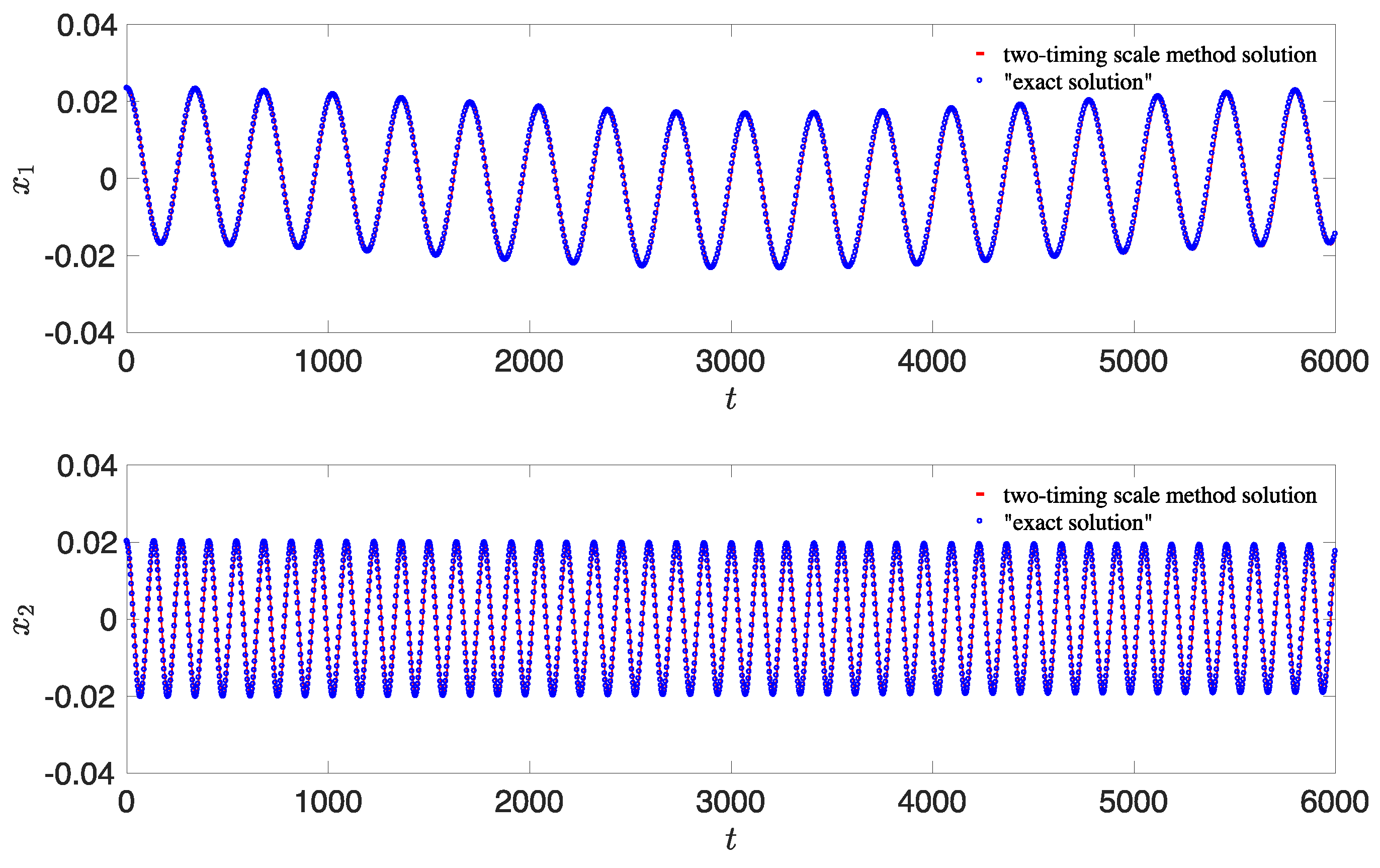
In order to verify the validity of the calculation results, a numerical comparison is carried out in this section. Consider the case and , and consequently . The initial value of the charged dilaton black hole system is selected as , and take the aforementioned integration constants and . As shown in Figure 1, the solution (28) obtained by the two-timing scale method is almost the same as the solution of the original system (14) (so-called “exact solution”) at each time. Meantime, these two solutions display the same trend as time evolves. In summary, these reveal that the two-timing scale method effectively describes this complex nonlinear charged dilaton black hole system, and the obtained asymptotic solutions are resultful with some parameter values.
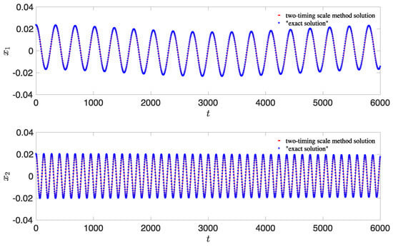
Figure 1.
A comparison between the two-timing scale method solution and the “exact solution” for , , , , , , , and .
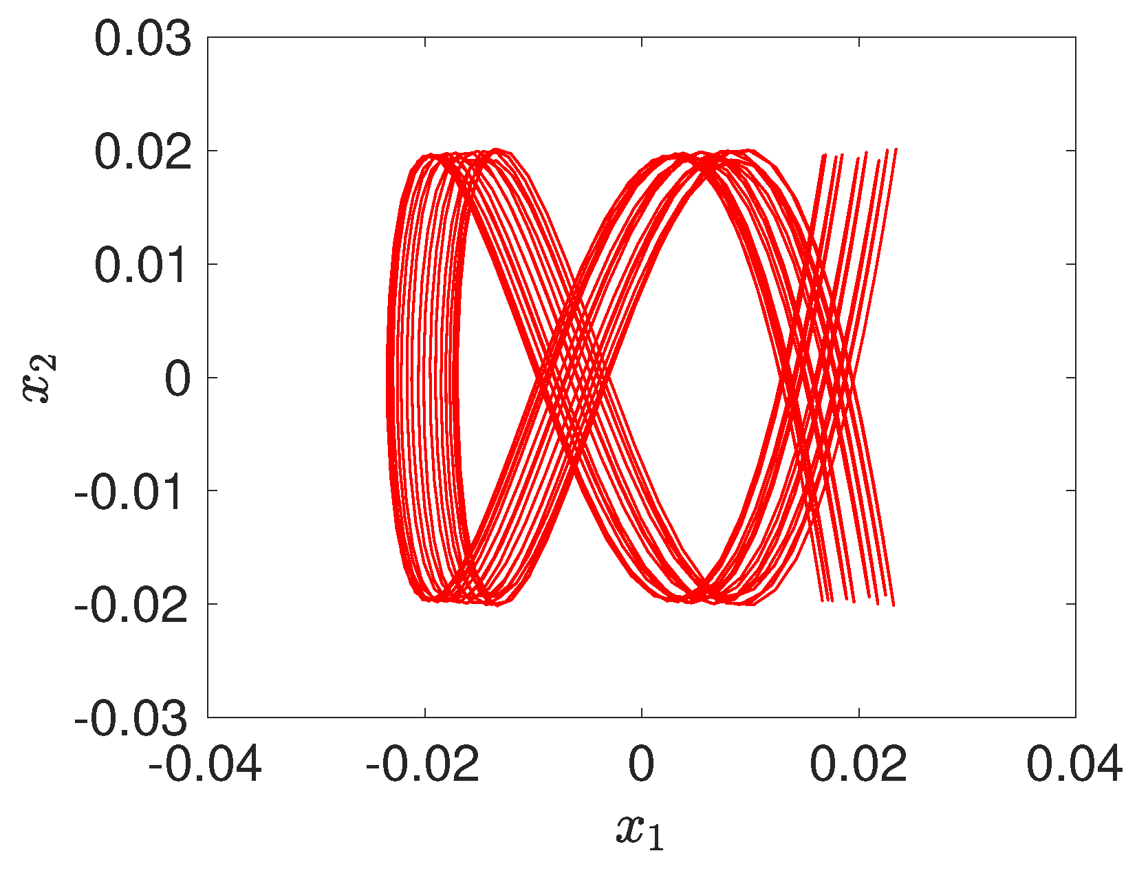
Moreover, at the same values of the above parameter, the phase portrait of the asymptotic solution is plotted as shown in Figure 2. Combining Figure 1 with Figure 2, it can be found that there exists a quasi-periodic motion, which is worthy of further study in the next section.
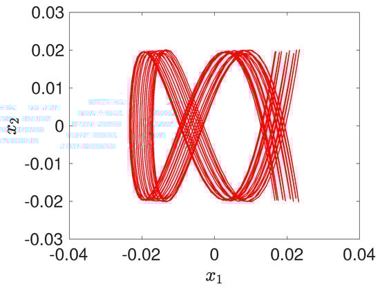
Figure 2.
Phase portrait of the two-timing scale method solution.
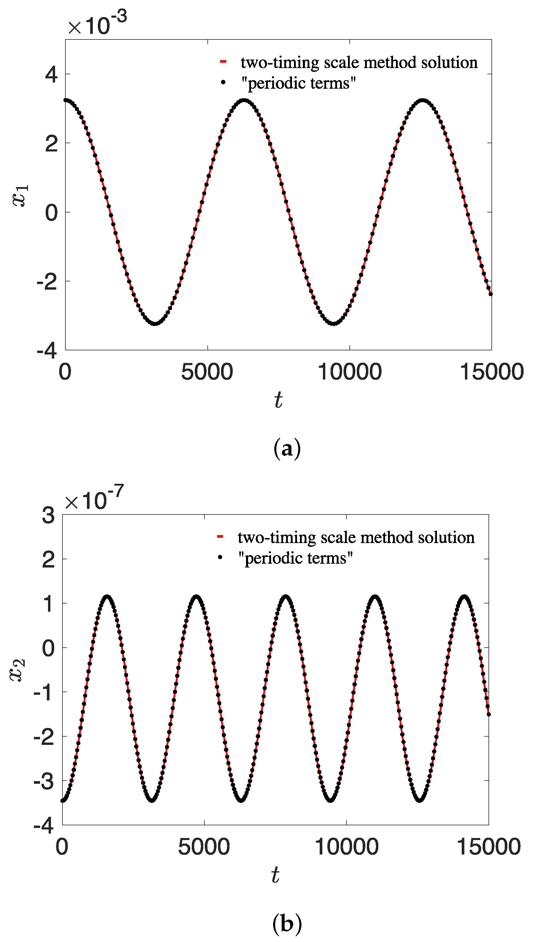
In order to explore the final state of the black hole flow, the following equations are considered by neglecting the non-periodic terms in the Equation (28), which are denoted by the “asymptotic periodic solutions”
Take , a comparison between the asymptotic solution and asymptotic periodic solution is shown in Figure 3. It is clear that the non-periodic terms in Equation (28) have barely any effect on the obtained solutions when the order of magnitude of integration constants is small.
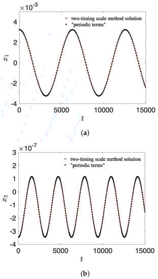
Figure 3.
A comparison between the asymptotic solution and asymptotic periodic solution for , , , , and : (a) Time-history diagram in -direction, (b) Time-history diagram in -direction.
5. Quasi-Periodic Behavior
Quasi-periodicity is a new type of long-term behavior, which is different from fixed point, homoclinic orbit, heteroclinic orbit, and periodic orbit. In deep space exploration, the Lissajous orbit and quasi-halo orbit near the Lagrangian points that have practical applications are also quasi-periodic. Mathematically, the frequencies in different directions are incommensurable, which implies that when the value of in Section 3 is an irrational number, the corresponding trajectory is said to be quasi-periodic. Then, as time evolves, the trajectory will never close into itself, which means that time-domain solutions will never be repeated. This is because any closed trajectory is bound to rotate an integer circle about and , the frequency ratio must be a rational number. On the contrary, each trajectory will be dense as time flows.
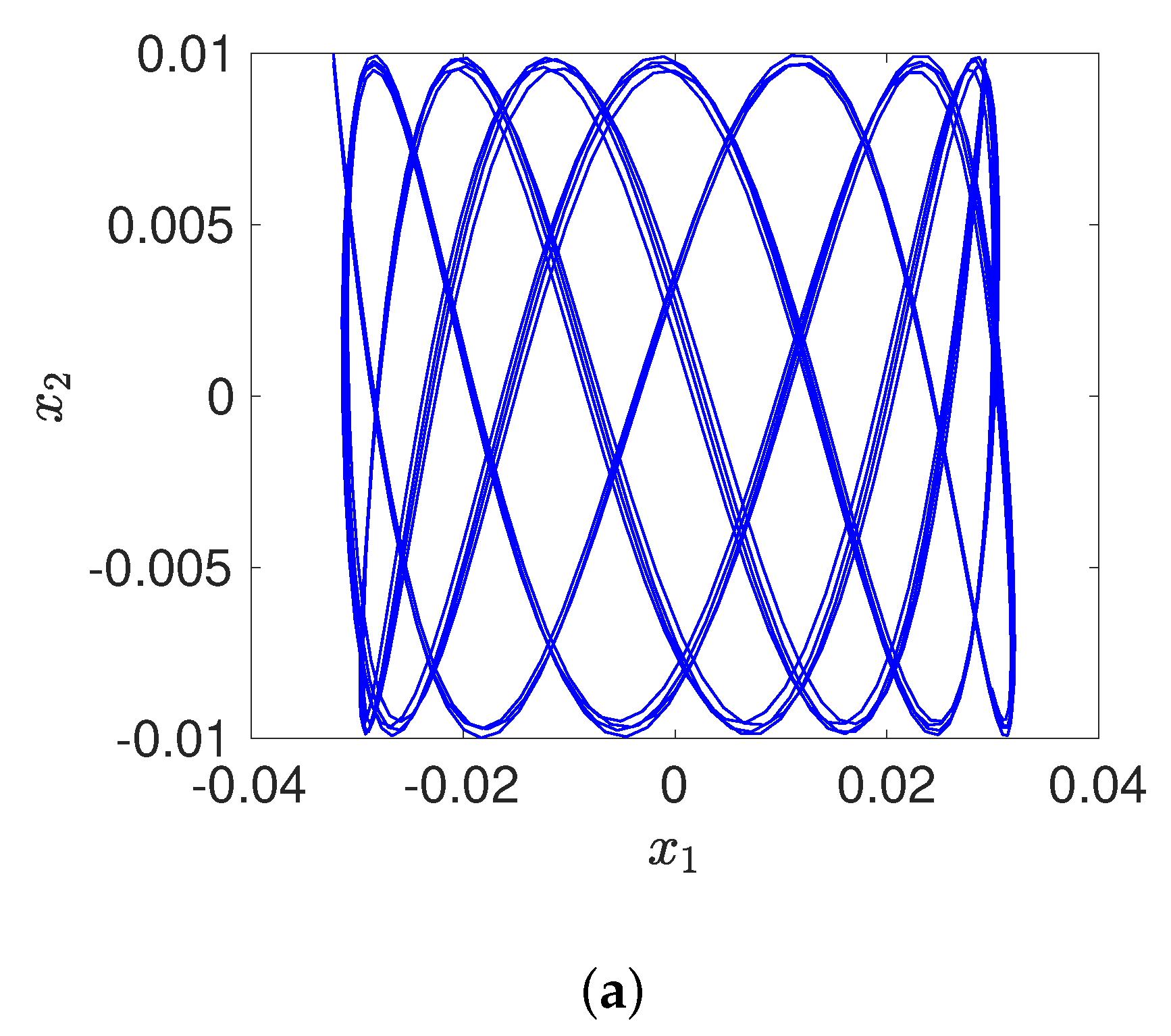
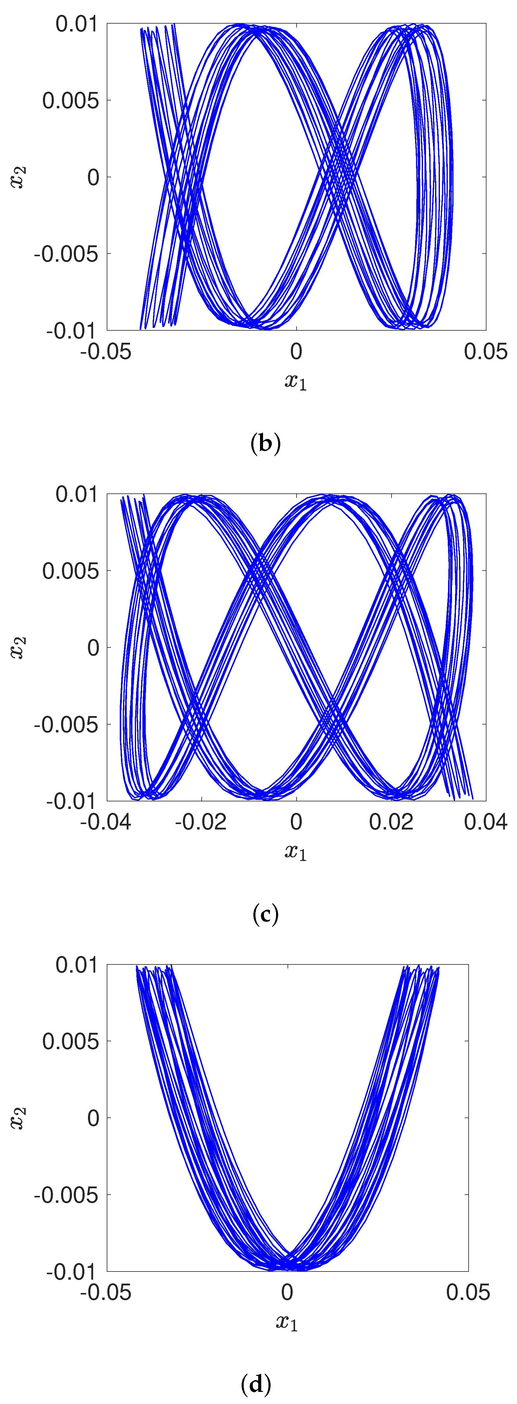
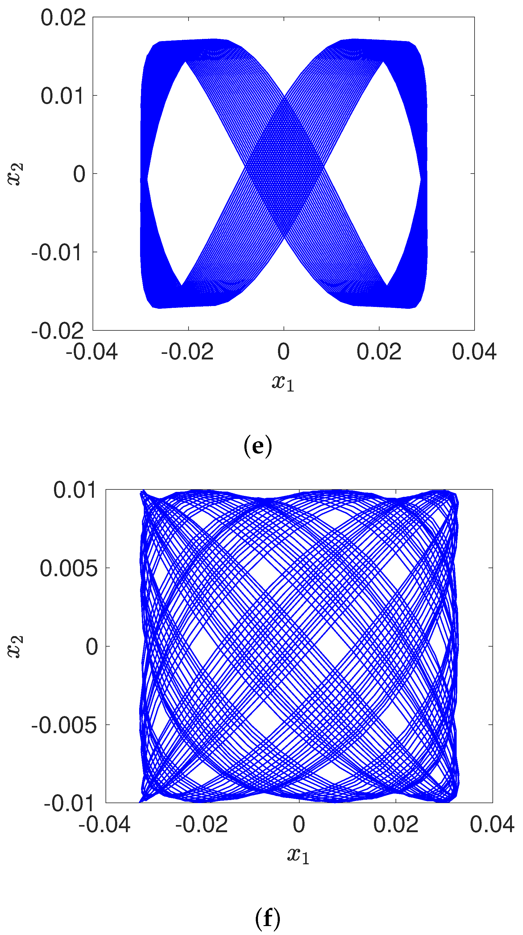
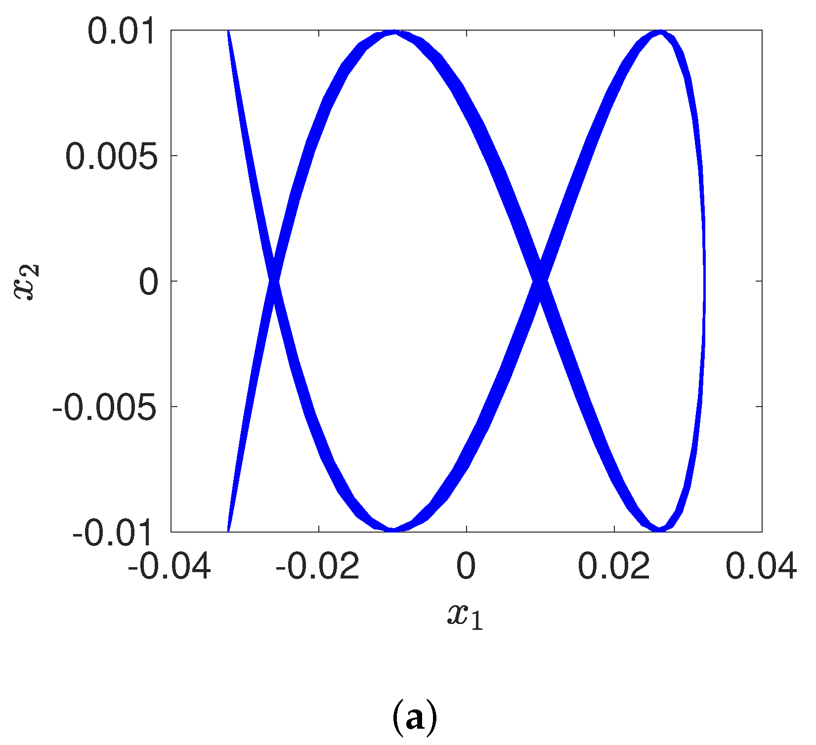
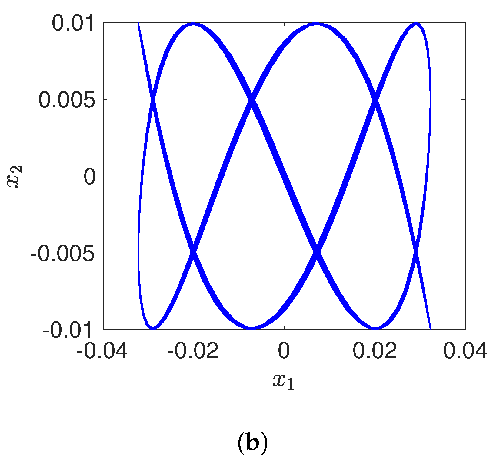
Based on the results in Section 4, it is worthy of studying the qualitative behavior of the “exact solution’’ of the charged dilaton black hole system (14). The quasi-periodic behavior characterized by the black hole flow is further studied in this section with different values of the parameters (see Table 1) and initial values of the black hole system. Note that the denominator of contains the irrational number ; then, it is obvious that there are constants and b to make an irrational number. Therefore,
is an irrational number for any rational constant . Then, several quasi-periodic motions are found and shown in Figure 4 and Figure 5. For example, take , , , , , , , , , and , and the initial value of the system as . Then, the phase portrait shows a “reticular shape” in Figure 4a, which characterizes the quasi-periodic motion of the black hole flow. In addition, seven more quasi-periodic motions are shown below, which are similar to “V-shape”, “8-shape” and “pillow-shape” and so on.

Table 1.
Parameter values in the charged dilaton black hole flow.
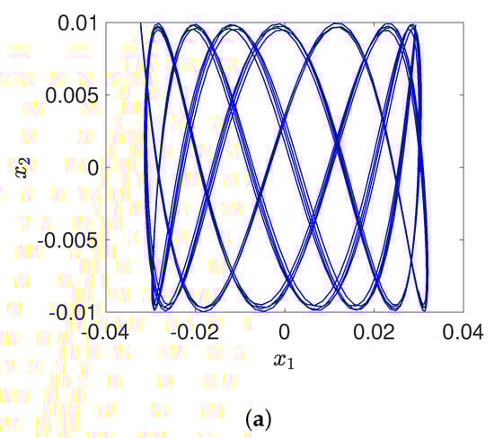
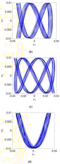
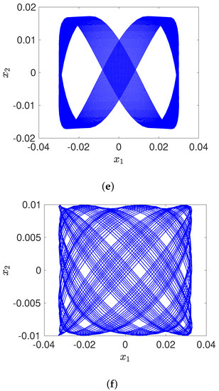
Figure 4.
(a–f) Phase portraits of the charged dilaton black hole system corresponding to the six groups in Table 1 when .
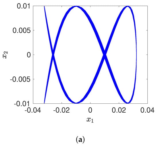
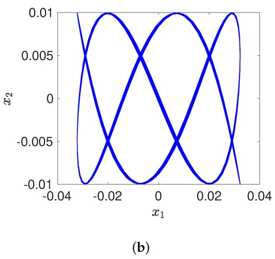
Figure 5.
(a,b) Phase portraits of the charged dilaton black hole system for different with .
Considering that the value of the thermal perturbation parameter is 0.000001, the related phase portraits of the system corresponding to the aforementioned Group (b) and Group (c) are shown in Figure 5. The phase trajectories of the system tend to be stable as time goes on. Moreover, the system’s motion tends to be periodic, and the vibration amplitude tends to be constant simultaneously.
6. Discussion and Conclusions
In this paper, the qualitative and quantitative analysis of charged dilation black holes is investigated. The two-timing scale method is applied to analyze the black hole flow equation and construct the second-order asymptotic analytical solution. According to these solutions, a numerical comparison with different system parameters values is carried out. By doing so, it can be found that these asymptotic solutions effectively describe the dynamical behavior of the black hole flow for a long time. At the same time, the relevant phase portraits are drawn to show quasi-periodic motion.
According to the obtained quasi-periodic motion, the quasi-periodic behavior of the black hole flow in the spinodal region is further studied when the frequency of is an irrational number. Several quasi-periodic motions with different parameter values are found. It is worth mentioning that when the thermal parameter perturbation takes a small value, the phase portraits of the black hole system exhibit better stability than the large value, and the vibration amplitude tends to be constant simultaneously.
Furthermore, to understand the final evolution state of the thermal dynamics of the black hole flow, the periodic solution is found according to the constructed analytical solution. The numerical comparison of these two solutions shows that they agree well for the small integral constant. In other words, the smaller the integral constant, the greater the extent of the black hole flow’s motion tends to be periodic.
Author Contributions
Conceptualization, F.G.; Formal analysis, R.W.; software, R.W.; writing-original draft, R.W.; writing—review and editing, F.G. All authors have read and agreed to the published version of the manuscript.
Funding
This research was funded by the National Natural Science Foundation of China (NSFC) through grant nos. 12172322 and 11672259, the China Scholarship Council through grant No. 201908320086, the Postgraduate Research & Practice Innovation Program of Jiangsu Province (KYCX21_3190).
Institutional Review Board Statement
Not applicable.
Informed Consent Statement
Not applicable.
Data Availability Statement
Not applicable.
Acknowledgments
We are very grateful to the anonymous reviewers whose comments and suggestions helped improve and clarify this paper.
Conflicts of Interest
The authors declare no conflict of interest.
Appendix A
References
- Oppenheimer, J.R.; Snyder, H. On continued gravitational contraction. Phys. Rev. 1939, 56, 455–459. [Google Scholar] [CrossRef] [Green Version]
- Webster, B.L.; Murdin, P. Cygnus X-1-a spectroscopic binary with a heavy companion? Nature 1972, 235, 37–38. [Google Scholar] [CrossRef]
- Campanelli, M.; Lousto, C.; Zlochower, Y.; Merritt, D. Large merger recoils and spin flips from generic black-hole binaries. Astrophys. J. 2007, 659, L5–L8. [Google Scholar] [CrossRef] [Green Version]
- Podsiadlowski, P.; Rappaport, S.; Han, Z. On the formation and evolution of black hole binaries. Mon. Not. R. Astron. Soc. 2010, 341, 385–404. [Google Scholar] [CrossRef] [Green Version]
- Abbott, B.P.; Abbott, R.; Abbott, T.D.; Abernathy, M.R.; Acernese, F.; Ackley, K.; Adams, C.; Adams, T.; Addesso, P.; Adhikari, R.X.; et al. Observation of gravitational waves from a binary black hole merger. Phys. Rev. Lett. 2016, 116, 061102. [Google Scholar] [CrossRef]
- Abbott, B.P.; Abbott, R.; Abbott, T.D.; Abernathy, M.R.; Acernese, F.; Ackley, K.; Adams, C.; Adams, T.; Addesso, P.; Adhikari, R.X.; et al. GW151226: Observation of gravitational waves from a 22-solar-mass binary black hole coalescence. Phys. Rev. Lett. 2016, 116, 241103. [Google Scholar] [CrossRef]
- Abbott, R.; Abbott, T.D.; Abraham, S.; Acernese, F.; Ackley, K.; Adams, A.; Adams, C.; Adhikari, R.X.; Adya, V.B.; Affeldt, C.; et al. Observation of gravitational waves from two neutron star-black hole coalescences. Astrophys. J. Lett. 2021, 915, L5. [Google Scholar] [CrossRef]
- Alexeyev, S.; Sendyuk, M. Black holes and wormholes in extended gravity. Universe 2020, 6, 25. [Google Scholar] [CrossRef] [Green Version]
- Stuchlík, Z.; Vrba, J. Epicyclic oscillations around Simpson-Visser regular black holes and wormholes. Universe 2021, 7, 279. [Google Scholar] [CrossRef]
- Kiritsis, E.; Kofinas, G. On Hořava-Lifshitz “black holes”. J. High Energy Phys. 2010, 2010, 122. [Google Scholar] [CrossRef] [Green Version]
- Poshteh, M.B.J.; Riazi, N. Phase transition and thermodynamic stability in extended phase space and charged Hořava-Lifshitz black holes. Gen. Relativ. Gravit. 2017, 49, 64. [Google Scholar] [CrossRef] [Green Version]
- Gao, F.B.; Llibre, J. Global dynamics of Hořava-Lifshitz cosmology with non-zero curvature and a wide range of potentials. Eur. Phys. J. 2020, 80, 137. [Google Scholar] [CrossRef]
- Król, J.; Klimasara, P. Black holes and complexity via constructible universe. Universe 2020, 6, 198. [Google Scholar] [CrossRef]
- Marto, J. Hawking radiation and black hole gravitational back reaction—A quantum geometrodynamical simplified model. Universe 2021, 7, 297. [Google Scholar] [CrossRef]
- Hawking, S.W. Black hole explosions? Nature 1974, 248, 30–31. [Google Scholar] [CrossRef]
- Hawking, S.W. Black holes and thermodynamics. Phys. Rev. D 1976, 13, 55–97. [Google Scholar] [CrossRef]
- Hawking, S.W.; Page, D.N. Thermodynamics of black holes in anti-de Sitter space. Commun. Math. Phys. 1983, 87, 577–588. [Google Scholar] [CrossRef]
- Wald, R.M. The thermodynamics of black holes. Living Rev. Relativ. 2001, 4, 6. [Google Scholar] [CrossRef] [Green Version]
- Hayward, S.A. Unified first law of black-hole dynamics and relativistic thermodynamics. Class. Quantum Gravity 1998, 15, 3147–3162. [Google Scholar] [CrossRef]
- Hendi, S.H.; Sajadi, S.N.; Khademi, M. Physical properties of a regular rotating black hole: Thermodynamics, stability, and quasinormal modes. Phys. Rev. D 2021, 103, 064016. [Google Scholar] [CrossRef]
- Gallerati, A. New black hole solutions in N=2 and N=8 gauged supergravity. Universe 2021, 7, 187. [Google Scholar] [CrossRef]
- Xiao, Y.; Chen, Y.; Feng, H.Y.; Zhu, C.R. Black hole solutions and thermodynamics in the infinite derivative theory of gravity. Phys. Rev. D 2021, 103, 044064. [Google Scholar] [CrossRef]
- Chamblin, A.; Emparan, R.; Johnson, C.V.; Myers, R.C. Holography, thermodynamics, and fluctuations of charged AdS black holes. Phys. Rev. D 1999, 60, 104026. [Google Scholar] [CrossRef] [Green Version]
- Wu, X.N. Multicritical phenomena of Reissner-Nordström anti-de Sitter black holes. Phys. Rev. D 2000, 62, 124023. [Google Scholar] [CrossRef]
- Dehghani, M.H.; Kamrani, S.; Sheykhi, A. P-V criticality of charged dilatonic black holes. Phys. Rev. D 2014, 90, 104020. [Google Scholar] [CrossRef] [Green Version]
- Zhang, M.; Yang, Z.Y.; Zou, D.C.; Xu, W.; Yue, R.H. P-V criticality of AdS black hole in the Einstein-Maxwell-power-Yang- Mills gravity. Gen. Relativ. Gravit. 2014, 47, 14. [Google Scholar] [CrossRef]
- Hu, Y.P.; Zeng, H.A.; Jiang, Z.M.; Zhang, H. P-V criticality in the extended phase space of black holes in Einstein- Horndeski gravity. Phys. Rev. D 2019, 100, 084004. [Google Scholar] [CrossRef] [Green Version]
- Hendi, S.H.; Dehghani, A. Criticality and extended phase space thermodynamics of AdS black holes in higher curvature massive gravity. Eur. Phys. J. C 2019, 79, 227. [Google Scholar] [CrossRef]
- Sharif, M.; Ama-Tul-Mughani, Q. P-V criticality and phase transition of the Kerr-Sen-AdS black hole. Eur. Phys. J. Plus 2021, 136, 284. [Google Scholar] [CrossRef]
- Liang, J. The P-v criticality of a noncommutative geometry-inspired Schwarzschild-AdS black hole. Chin. Phys. Lett. 2017, 34, 080402. [Google Scholar] [CrossRef]
- Chen, S.B.; Liu, X.F.; Liu, C.Q. P-V criticality of an AdS black hole in f(R) gravity. Chin. Phys. Lett. 2013, 30, 060401. [Google Scholar] [CrossRef] [Green Version]
- Liang, J.; Guan, Z.H.; Liu, Y.C.; Liu, B. P-v criticality in the extended phase space of a noncommutative geometry inspired Reissner-Nordström black hole in AdS space-time. Gen. Relativ. Gravit. 2017, 49, 29. [Google Scholar] [CrossRef]
- Li, R.; Wang, J. Hawking radiation and P-v criticality of charged dynamical (Vaidya) black hole in anti-de Sitter space. Phys. Lett. B 2021, 813, 136035. [Google Scholar] [CrossRef]
- Zhao, H.H.; Zhang, L.C.; Zhao, R. Two-phase equilibrium properties in charged topological dilaton AdS black holes. Adv. High Energy Phys. 2016, 2016, 2021748. [Google Scholar] [CrossRef]
- Sherkatghanad, Z.; Mirza, B.; Mirzaiyan, Z.; Mansoori, S.A.H. Critical behaviors and phase transitions of black holes in higher order gravities and extended phase spaces. Int. J. Mod. Phys. D 2017, 26, 1750017. [Google Scholar] [CrossRef] [Green Version]
- Hendi, S.H.; Nemati, A.; Lin, K.; Jamil, M. Instability and phase transitions of a rotating black hole in the presence of perfect fluid dark matter. Eur. Phys. J. C 2020, 80, 296. [Google Scholar] [CrossRef] [Green Version]
- Dehyadegari, A.; Sheykhi, A.; Montakhab, A. Novel phase transition in charged dilaton black holes. Phys. Rev. D 2017, 96, 084012. [Google Scholar] [CrossRef] [Green Version]
- Liang, K.; Wang, P.; Wu, H.; Yang, M. Phase structures and transitions of Born-Infeld black holes in a grand canonical ensemble. Eur. Phys. J. C 2020, 80, 187. [Google Scholar] [CrossRef] [Green Version]
- Ma, Y.; Zhang, Y.; Zhang, L.; Wu, L.; Gao, Y.; Cao, S.; Pan, Y. Phase transition and entropic force of de Sitter black hole in massive gravity. Eur. Phys. J. C 2021, 81, 42. [Google Scholar] [CrossRef]
- Chabab, M.; El Moumni, H.; Iraoui, S.; Masmar, K. Phase transitions and geothermodynamics of black holes in dRGT massive gravity. Eur. Phys. J. C 2019, 79, 342. [Google Scholar] [CrossRef]
- Hendi, S.H.; Azari, F.; Rahimi, E.; Elahi, M.; Owjifard, Z.; Armanfard, Z. Thermodynamics and the phase transition of topological dilatonic Lifshitz-like black holes. Ann. Der Phys. 2020, 532, 2000162. [Google Scholar] [CrossRef]
- Wang, P.; Wu, H.W.; Yang, H.T. Thermodynamics and phase transition of a nonlinear electrodynamics black hole in a cavity. J. High Energy Phys. 2019, 2019, 002. [Google Scholar] [CrossRef] [Green Version]
- Wang, P.; Wu, H.W.; Yang, H.T. Thermodynamics and phase transitions of nonlinear electrodynamics black holes in an extended phase space. J. Cosmol. Astropart. Phys. 2019, 2019, 052. [Google Scholar] [CrossRef] [Green Version]
- Zhang, L.C.; Ma, M.S.; Zhao, H.H.; Zhao, R. Thermodynamics of phase transition in higher-dimensional Reissner-Nordström-de Sitter black hole. Eur. Phys. J. C 2014, 74, 3052. [Google Scholar] [CrossRef] [Green Version]
- Qiu, J.H.; Gao, C.J. Constructing higher-dimensional exact black holes in Einstein-Maxwell-scalar theory. Universe 2020, 6, 148. [Google Scholar] [CrossRef]
- Guo, X.Y.; Li, H.F.; Zhang, L.C.; Zhao, R. Continuous phase transition and microstructure of charged AdS black hole with quintessence. Eur. Phys. J. C 2020, 80, 168. [Google Scholar] [CrossRef] [Green Version]
- Chen, Y.; Li, H.T.; Zhang, S.J. Chaos in Born-Infeld-AdS black hole within extended phase space. Gen. Relativ. Gravit. 2019, 51, 134. [Google Scholar] [CrossRef] [Green Version]
- Dai, C.Q.; Chen, S.B.; Jing, J.L. Thermal chaos of a charged dilaton-AdS black hole in the extended phase space. Eur. Phys. J. C 2020, 80, 245. [Google Scholar] [CrossRef]
- Chabab, M.; El Moumni, H.; Iraoui, S.; Masmar, K.; Zhizeh, S. Chaos in charged AdS black hole extended phase space. Phys. Lett. B 2018, 78, 316–321. [Google Scholar] [CrossRef]
- Mahish, S.; Bhamidipati, C. Chaos in charged Gauss-Bonnet AdS black holes in extended phase space. Phys. Rev. D 2019, 99, 106012. [Google Scholar] [CrossRef] [Green Version]
- Tang, B. Temporal and spatial chaos in the Kerr-AdS black hole in an extended phase space. Chin. Phys. C 2021, 45, 055101. [Google Scholar] [CrossRef]
- Guo, X.; Liang, K.; Mu, B.; Wang, P.; Yang, M. Chaotic motion around a black hole under minimal length effects. Eur. Phys. J. C 2020, 80, 745. [Google Scholar] [CrossRef]
- Zhou, X.; Chen, S.B.; Jing, J.L. Chaotic motion of scalar particle coupling to Chern-Simons invariant in Kerr black hole spacetime. Eur. Phys. J. C 2021, 81, 233. [Google Scholar] [CrossRef]
- Shafiq, S.; Hussain, S.; Ozair, M.; Aslam, A.; Hussain, T. Charged particle dynamics in the surrounding of Schwarzschild anti-de Sitter black hole with topological defect immersed in an external magnetic field. Eur. Phys. J. C 2020, 80, 744. [Google Scholar] [CrossRef]
- Hussain, S.; Hussain, I.; Jamil, M. Dynamics of a charged particle around a slowly rotating Kerr black hole immersed in magnetic field. Eur. Phys. J. C 2014, 74, 3210. [Google Scholar] [CrossRef] [Green Version]
- Strogatz, S.H. Nonlinear Dynamics and Chaos; CRC Press, Taylor & Francis Group: Boca Raton, FL, USA, 2018. [Google Scholar]
- Sheykhi, A. Thermodynamics of charged topological dilaton black holes. Phys. Rev. D 2007, 76, 124025. [Google Scholar] [CrossRef] [Green Version]
- Sheykhi, A. Topological Born-Infeld-dilaton black holes. Phys. Lett. B 2008, 662, 7–13. [Google Scholar] [CrossRef] [Green Version]
- Slemrod, M.; Marsden, J.E. Temporal and spatial chaos in a van der Waals fluid due to periodic thermal fluctuations. Adv. Appl. Math. 1985, 6, 135–158. [Google Scholar] [CrossRef] [Green Version]
- Melnikov, V.K. On the stability of the center for time periodic perturbations. Trans. Mosc. Math. Soc. 1963, 12, 3–52. [Google Scholar]
Publisher’s Note: MDPI stays neutral with regard to jurisdictional claims in published maps and institutional affiliations. |
© 2021 by the authors. Licensee MDPI, Basel, Switzerland. This article is an open access article distributed under the terms and conditions of the Creative Commons Attribution (CC BY) license (https://creativecommons.org/licenses/by/4.0/).