Two-Dimensional Correlation Function of Binary Black Hole Coalescences

Abstract

We compute the two-dimensional correlation functions of the binary black hole coalescence detections in LIGO-Virgo’s first and second observation runs. The sky distribution of binary black hole coalescence events is tested for correlations at different angular scales by comparing the observed correlation function to two reference functions that are obtained from mock datasets of localization error regions uniformly distributed in the sky. No excess correlation at any angular scale is found. The power-law slope of the correlation function is estimated to be $\gamma =2.24\pm 0.33$ at the three-$\sigma$ confidence level, a value consistent with the measured distribution of galaxies.

1. Introduction

On 14 September 2015, researchers from the Laser Interferometer Gravitational-wave Observatory (LIGO) [1] Scientific Collaboration (LSC) and the European Virgo Collaboration [2] made the first direct detection of Gravitational Waves (GWs) from a pair of coalescing black holes [3]. Less than two years after that first announcement, LIGO and Virgo observed GWs from the merger of two neutron stars [4], an event that was rapidly followed by the Fermi Gamma-ray Space Telescope’s detection of a gamma-ray flash, and eventually by optical, infrared, radio, and X-ray observations by hundreds of telescopes around the world in what became the most observed event in the history of modern astronomy [5].

Currently, GW astronomy is a well-established scientific discipline. In the first two observing runs of Advanced LIGO and Virgo, O1 and O2, LSC and Virgo collaboration researchers observed ten Binary Black Hole (BBH) coalescence detections and one binary neutron star coalescence detection. The third observation run, O3, brought us candidate detections on a weekly basis [6], enabling a plethora of novel astrophysical and theoretical investigations.

The next decade will see GW astronomy further expand its reach in frontier scientific research. Japan’s KAGRA detector [7] has joined the international network of GW ground-based observatories. India has established the LIGO-India Scientific Collaboration (LISC) and finalized plans for the construction of the LIGO-India detector [8]. The European space-based LISA mission [9], slated to launch in 2034, will greatly improve detection capabilities and localizations of astrophysical sources. The International Pulsar Timing Array project will detect ultra-low frequency GWs within ten years [10]. Optical, particle, and GW astronomy will together explore the Universe through complementary physical carriers.

The publication of LIGO-Virgo’s first catalog of compact binary merger signals [11] has shown that GW astrophysics is a powerful tool for population and source property studies of compact objects, tests of General Relativity, and large-scale cosmological measurements. However, many open questions still remain. For example, tests of GR have returned a null result [12]; the formation channels of black hole binaries [13] and the physics of EM-bright mergers [14] are still unclear, as well as the determination of the Hubble constant from GW sirens [15]. Despite LIGO and Virgo running all-sky, unmodeled searches [16,17], no GW signal has been detected that cannot be modeled as a compact binary coalescence. Other sources of multi-messenger signals such as isolated compact objects [18], core-collapse supernovae [19], and magnetars [20] have not been observed in the GW domain.

The rapid growth in the number of BBH coalescence detections and the dramatic improvement in their sky localizations are turning GW astrophysics into a precision observational science like large-scale structure astrophysics and early-Universe cosmology. One important physical concept in large-scale structure investigations and observational cosmology is that of the Correlation Function (CF) [21]. The (two-point) (auto-)CF describes the excess probability of finding pairs of points at a given separation. In large-scale astrophysics and observational cosmology, the CF (or its homolog in the frequency space, the power spectrum) is commonly used to describe the spatial distribution of galaxies or the density fluctuations observed in the cosmic microwave background. The CF from galaxy surveys, for example, allows astronomers to estimate the distance scales of galaxy clustering and gain information about the origin and evolution of the Universe’s large-scale structures.

The purpose of this short article is to introduce the concept of the CF for BBH coalescence events. We use the public BBH coalescence detections in LIGO-Virgo’s O1 and O2 runs to compute the two-dimensional CF for the population of these objects. Ten detections with sky localizations ranging from 39 square degrees to 1666 square degrees are clearly not sufficient to draw any meaningful conclusion on the spatial distribution of BBH coalescences. However, this calculation shows that the CF can be used to investigate the statistical properties of the population of these objects. We illustrate the method by comparing the two-dimensional CF obtained from the LIGO-Virgo O1-O2 BBH detections to a CF obtained by a random distribution of the same detections. The result shows that the two-dimensional spatial distribution of the detections is consistent with an isotropic distribution, as reported in Ref. [22] by implementing a pixelization-based method for the O1-O2 BBH detections. We also confirm this conclusion by comparing the CF to a synthetic CF obtained by simulating a number of BBH detections with sky localization error regions consistent with those of the LIGO-Virgo sample.

2. Two-Dimensional Correlation Function

In our analysis, we follow the customary definition for the two-dimensional (angular) CF of large-scale astrophysics [21]. The two-dimensional CF of a population of objects describes the excess probability of finding two objects separated by the angular distance $\theta$ with respect to a uniform distribution. To compute the CF of the BBH population, we treat the sky localization error regions of the BBH detections as probability density heat maps. Given the (normalized) sky localization error region map of the $i^{\mathrm{th}}$ BBH detection in the sample, $M_i(\chi ,\phi )$, where $\chi$ and $\phi$ are the polar and azimuthal angles on the celestial sphere, respectively, we define the sky localization probability density map of the sample as:

$$M(\chi ,\phi )=\frac{1}{A\left(N\right)}\sum _{i=1}^N{F}_i(\chi ,\phi )M_i(\chi ,\phi ),$$

(1)

where N is the number of BBH detections, $F_i$ are probability weights that depend on the GW detector network sensitivity, and $A\left(N\right)$ is a normalization factor. By expanding the sky localization map in spherical harmonics,

$$M(\chi ,\phi )=\sum _{lm}{a}_{lm}{Y}_{lm}(\chi ,\phi ),$$

(2)

the sky correlation function of the BBH sample can be defined as:

$$C\left(\theta \right)={\langle M\left({\widehat{n}}_1\right)·M\left({\widehat{n}}_2\right)\rangle }_{21},$$

(3)

where the average is taken over the observed sky with angular separation $\theta$ held fixed. Using the addition theorem of spherical harmonics, the CF can be written as:

$$C\left(\theta \right)=\frac{1}{4\pi }\sum _l{a}_l^2{P}_l(cos\theta ),$$

(4)

where $P_l(cos\theta )$ denotes the Legendre polynomial of order l and argument $cos\theta$, and we have defined $a_l^2={\sum }_m{\left|a_{lm}\right|}^2$. Note that the CF in Equation (4) differs with the usual definition of the angular power spectrum that is used in Cosmic Microwave Background (CMB) cosmology, where $a_l^2=(2l+1)C_l$. As the map $M(\chi ,\phi )$ describes a probability density field, rather than the perturbation field of a physical quantity, in the following, we focus on the CF instead of the power spectrum, which is the standard measure for fluctuation fields.

The quantities $a_l^2$ are measured from the sky localization map $M(\chi ,\phi )$ and determine the two-dimensional angular distribution of the BBH sample. Comparison of the CF to theoretical models involves modification of Equation (4) by multiplying the $a_l^2$ coefficients by a window function $W_l$ to take into account experimental constraints in the observations. For example, the finite beam resolution of the detector introduces a high-l cutoff that can be modeled with a window function $W_l\propto exp[-l(l+1){\sigma }^2]$, where $\sigma$ is the detector resolution [21]. If the object population cannot be observed across the full sky, a mask is required. In contrast with CMB observations, where the region of the sky along the galactic plane must be masked in CMB observations due to the impossibility of measuring temperature fluctuations along the galactic plane, the full sky is transparent to GWs, and no mask is necessary. As the sky map in Equation (1) is obtained by summing the sky localization error regions of the BBH detections, the angular resolution is determined by the diffraction-limited spot size of the LIGO detectors:

$${\theta }_{\mathrm{res}}=\frac{c}{2df},$$

(5)

where d is the typical separation of the detectors in the network, c is the speed of light, and f is the frequency of the measurement. Assuming a typical frequency of 200 Hz for the detector sensitivity and a LIGO-Virgo detector distance $d\sim 7000$ km, a crude estimate of the minimum map angular resolution is ${\theta }_{\mathrm{res}}\sim 3^{°}$, or $\sigma \sim 1/30$, implying a high-l cut-off of $l_{\max }\sim 30$.

In the following analysis, for the sake of simplicity, we assume the probability weights in Equation (1) to be constant, i.e., we assume that the sensitivity of the LIGO-Virgo detector network does not depend on the sky position (see Ref. [22] for a more refined analysis and a discussion on the effects of detector sensitivity on isotropic test of GW detections). An additional, possible modification of Equation (4) is due to the different sensitivities of the GW detector network across the O1-O2 epochs and the varying number of detectors observing each BBH event in the sample. These systematics can be eliminated, at least partially, by comparing the observed CF $C_{\mathrm{obs}}\left(\theta \right)$ to a CF, which is computed from a set of $\mathcal{N}$ reference maps $M_{\mathrm{ref},k}(\chi ,\phi )$, $k=1,\cdots \mathcal{N}$, obtained by uniformly distributing the observed BBH sky localization error regions in the sky. A more refined analysis could be performed by injecting a population of simulated BBH signals with a uniform angular distribution and then creating the reference map by recovering the sky localization error regions of these injections with the GW network in the same configuration as in the real case. While this procedure would produce a more rigorous CF estimate than the one considered here, we consider it beyond the scope of this paper due to the small sample of BBH detections and the illustrative purpose of our analysis. We plan to revisit this procedure in a future work.

3. Results

We used the public sky localizations of the O1-O2 LIGO-Virgo BBH detections from the GW Open Science Center [23] and the open source Healpy package [24] to compute the CF. The sky localization error regions of the BBH detections came with different resolutions. We first rescaled each map to an NSIDE resolution of 256, corresponding to a pixel angular resolution of ${\theta }_{\mathrm{pix}}\sim {0.23}^{°}\ll {\theta }_{\mathrm{res}}$. Choosing different values of the map resolution affected the final results only by a few percent. We then created the map $M_{\mathrm{obs}}(\chi ,\phi )$ in Equation (1) by summing the sky localization error regions of each BBH event and normalizing to the number of detections, such as ${\sum }_j{M}_{\mathrm{obs}}\left(p_j\right)=1$, where $p_j$ denotes the $j^{\mathrm{th}}$ pixel. 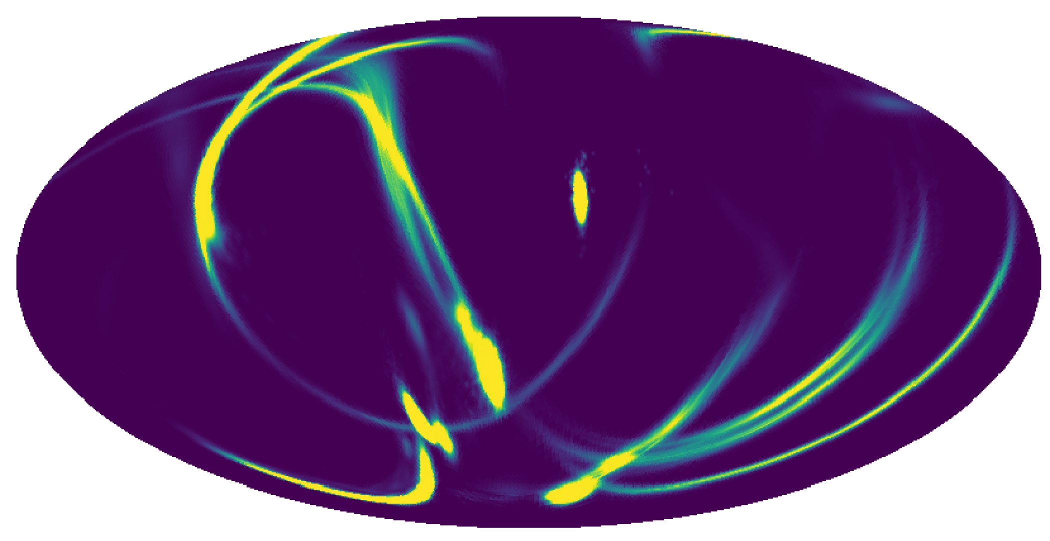A Mollweide representation of $M_{\mathrm{obs}}(\chi ,\phi )$ in Equation (1) is shown in Figure 1.

The $M_{\mathrm{obs}}(\chi ,\phi )$ map was treated as a heat map, and the Healpy function map2alm was used to compute $a_{lm}$. The coefficients of the Legendre expansion in Equation (4) were then obtained by summing the $|a_{lm}{|}^2$ in m. We followed the same procedure to compute the CF from reference maps $M_{\mathrm{ref},k}(\chi ,\phi )$ used to test possible angular correlation signatures in the CF.

In our analysis, we compared the observed CF $C_{\mathrm{obs}}\left(\theta \right)$ to two reference CFs. The first CF (Model A), $C_{\mathrm{ref},A}\left(\theta \right)$, was obtained by averaging the CF of 500 artificial maps, each obtained by randomly rotating the maps of each single BBH detection in the sky by arbitrary $\chi$ and $\phi$ angles. The second CF (Model B), $C_{\mathrm{ref},B}\left(\theta \right)$, was obtained by averaging 500 synthetic maps, each consisting of 10 elliptically-shaped sky localization error regions with random orientation and uniformly distributed in the sky. The sky localization areas of these artificial events were chosen such that their semi-axes were $R·(x,1/x)$, where x is uniformly distributed in $(0,10)$, and their area $\pi R^2$ was drawn from a lognormal distribution with mean (standard deviation) equal to the mean (standard deviation) of the sky localization areas of the observed events. Probability distribution contours of each of these artificial sky localization areas were simulated by superimposing 100 regions built as described above and radius decreasing as $f_n\left(R\right)=Rln\left(2\right)/ln(2+n)$, where $n=0\cdots 99$. The above parameters reproduced sky localization error regions qualitatively similar to the observed BBH error regions while their variations did not significantly affect the final CF. Both reference maps were normalized to the number of detections in the sample, following the same procedure used for the observed map. One example of a synthetic map is shown in Figure 2.

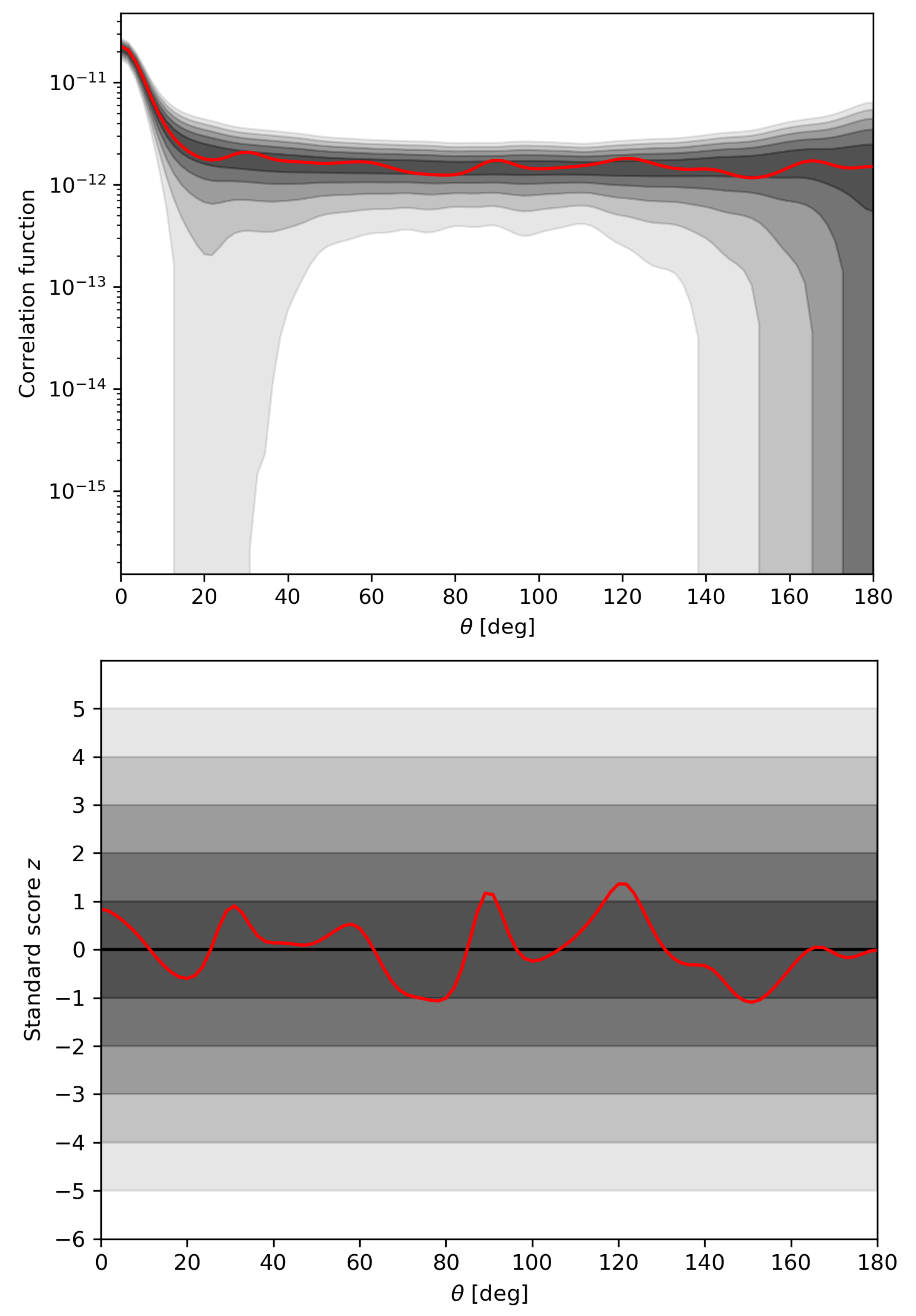
Figure 3 shows the observed CF compared to the reference CF for Model A. $C_{\mathrm{obs}}\left(\theta \right)$ is represented in the top plot by the red curve. The five grey-shaded bands denote one through five standard deviations from the average of the CF computed on the reference maps $M_{\mathrm{ref},k}(\chi ,\phi )$ from Model A, $C_{\mathrm{ref},A}\left(\theta \right)$. The bottom plot shows $C_{\mathrm{obs}}\left(\theta \right)$ normalized to $C_{\mathrm{ref},A}\left(\theta \right)$. The observed CF lies entirely in the two-$\sigma$ band of the reference map, thus showing no excess correlation at any angular scale with respect to a uniform sky distribution of the O1-O2 detections. 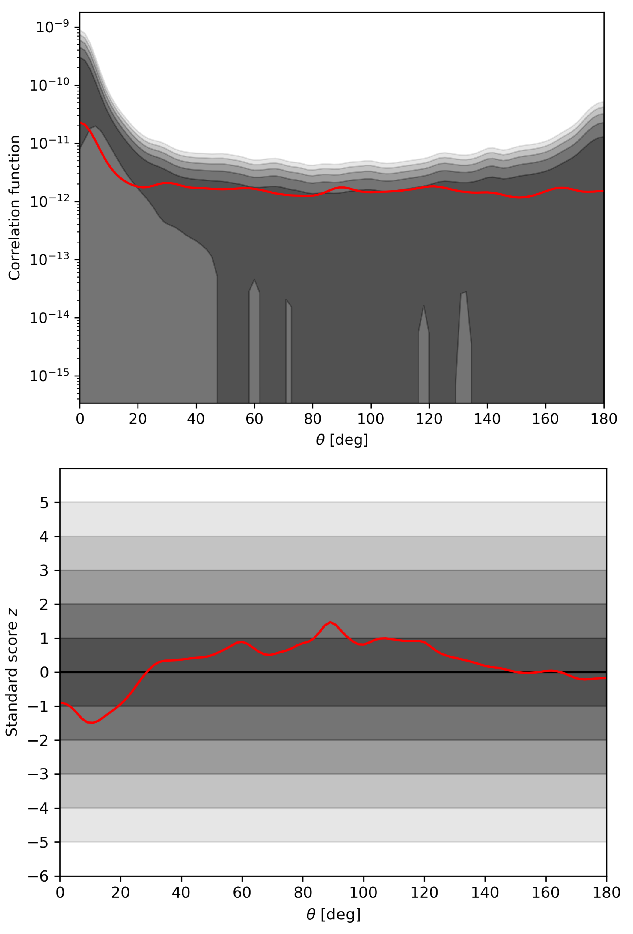No excess correlation at any angular scale could be found when comparing $C_{\mathrm{obs}}\left(\theta \right)$ to the reference CF for Model B, $C_{\mathrm{ref},B}\left(\theta \right)$. Results for this model are shown in Figure 4. The observed CF lied entirely within the 2-$\sigma$ error band of $C_{\mathrm{ref},B}\left(\theta \right)$. At small angular scales, $C_{\mathrm{obs}}\left(\theta \right)$ showed a lack of correlation compared to $C_{\mathrm{ref},B}\left(\theta \right)$. This mismatch was likely due to the crude approximation used to simulate the artificial maps. As can be seen from Figure 1, the LIGO-Virgo sky localization error regions of observed BBH events are not perfect ellipses. Even if they were, their ellipticity would not follow a uniform distribution in their semi-axis ratio. Finally, drawing samples from a lognormal distribution of sky localization areas did not accurately represent the observed distribution of sky localizations in O1 and O2. A much more accurate estimate of BBH events’ angular correlations could be obtained by simulating realistic sky maps by injecting, recovering, and localizing events according to the actual sensitivity of the GW detector network.

The CF in Equation (4) can be interpreted as a weighted projection of the spatial two point CF $\xi \left(r\right)$. At small scales, the power-law behavior of the CF is expected to be:

$$C\left(\theta \right)={\left(\frac{\theta }{{\theta }_0}\right)}^{1-\gamma },$$

(6)

where ${\theta }_0$ is an angular correlation scale and $\gamma$ is the power-law slope of the spatial two point CF:

$$\xi \left(r\right)={\left(\frac{r}{r_0}\right)}^{-\gamma },$$

(7)

where $r_0$ is the spatial correlation length. The power-law slope of the BBH distribution can be obtained by fitting $C_{\mathrm{obs}}\left(\theta \right)$ at small angular scales. A weighted best fit of Equation (6) from $\theta \sim {\theta }_{\mathrm{res}}$ to $\theta \sim {18}^{°}$, where departures from the power-law behavior become evident, gives for the power-law slope $\gamma =2.24\pm 0.33$ at three-$\sigma$ confidence level, a value consistent with a uniform distribution of objects, $\xi \left(r\right)\sim r^{-2}$. As a comparison, the power-law slope from Sloan Digital Sky Survey (SDSS) data is $\gamma \sim 1.8$ over the range ${0.005}^{°}$–${10}^{°}$ [25]. The VIMOS Public Extragalactic Redshift Survey (VIPERS) reports $\gamma \sim 1.7-1.8$ for a broad range of galaxy luminosities and stellar masses in the redshift range $0.5<z<1.1$ [26]. The VIMOS-VLT Deep Survey observes a significant redshift evolution of the luminosity dependence of the power-law slope parameter with $\gamma$ steepening from $\gamma \sim 1.7$ at low redshift to $\gamma \sim 2.4$ for $z\sim 0.9$ and galaxies with high intrinsic luminosity [27]. In contrast to the SDSS, VIPERS, and VIMOS-VLT results, which point to galaxy clustering in the redshift range of BBH detections, $z\lesssim 0.5$, our result showed no evidence of clustering at these distance scales. It would be interesting to test whether any evidence of clustering would appear in the data with more BBH detections and better sample statistic.

4. Conclusions

In this short article, we computed the two-dimensional CF of BBH observations in the first and second observation runs of advanced LIGO and Virgo. The CF is commonly used in large-scale structure astrophysics and precision cosmology to quantify the spatial distribution of an object class population. Similarly, we used the two-dimensional CF to measure the statistical properties of the BBH coalescence spatial distribution. By comparing the CF of the LIGO-Virgo detections to a simulated CF from a synthetic sample of sky localizations and a CF obtained by randomly re-orienting the BBH detections, we showed that the distribution of O1-O2 BBH events in the sky was in agreement with a uniform distribution of sources, as previously reported in Ref. [22]. The power-law slope of the CF was found to be $\gamma =2.24\pm 0.33$, a value consistent with the upper bound of the power-law slope from galaxy surveys at low redshift z.

While the limited number of O1-O2 detections with large sky localization error regions did not allow us to draw any significant physical conclusions, our work lays the formalism for computing the CF of a class of GW detections. Our analysis was clearly rudimentary and could be improved in many ways. The extension to the tens of LIGO-Virgo detections in O3 is straightforward. A better estimate for the two-dimensional spatial distribution of BBH coalescence events could be obtained by comparing the detected CF to a synthetic CF from a realistic population of events as done in Ref. [22]. This could be done by testing the detected CF against a CF from injection sets consistent with the observed BBH coalescence population and detector network sensitivity. The existence of angular correlations in the spatial distribution of BBH coalescences could be tested by building CFs for events distributed isotropically in the sky, or at given angular scales. Comparisons of the observed BBH CF to CFs of anisotropic models for the astrophysical GW background [28] and other astrophysical objects could be used to test correlations of BBH events with the spatial distribution of these objects [29], test BBH population paradigms, and probe fundamental physics [30,31]. Our method could also be extended to include information about the distances of the BBH sources by computing the three-dimensional CF [32]. The latter could be compared to CFs obtained from given models of population synthesis, as well as three-dimensional CFs of other astrophysical objects. With the anticipated higher rate of detections and more accurate sky localizations in future LIGO-Virgo observing runs, the CF of BBH and other GW-bright sources may prove itself as another useful tool for GW astronomy investigations.