Article

Significance of Black Hole Visualization and Its Implication for Science Education Focusing on the Event Horizon Telescope Project

1
Department of Science Education, Chuncheon National University of Education, Chuncheon, Gangwon-do 24328, Korea
2
The Center for Educational Research, Seoul National University, Seoul 08826, Korea
3
Department of Physics Education, Chungbuk National University, Cheongju, Chungbuk 28644, Korea
*
Author to whom correspondence should be addressed.
Universe 2020, 6(5), 70; https://doi.org/10.3390/universe6050070
Submission received: 18 April 2020 / Revised: 18 May 2020 / Accepted: 22 May 2020 / Published: 25 May 2020
(This article belongs to the Special Issue Black Holes and Relativistic Jets)

Abstract

:
In recent years, substantial progress has been made in black hole visualization. However, there is a lack of essential up-to-date information regarding black holes in current school curricula, in spite of students’ substantial interest in black holes. In this study, we examined the implications of the Event Horizon Telescope project, a recent achievement of the scientific community, for science education. An analysis of the black hole visualization research process, based on Giere’s scientific reasoning model, revealed that there are two categories of the black hole visualization processes: visualization through prediction based on a theory and visualization through real-world observation data. Black hole images are not merely scientific outputs that students must memorize; rather, they can be a useful resource for learning the nature of science and the characteristics of scientific reasoning.

1. Introduction

Scientists have continuously sought to visualize the invisible domain, including the micro world, such as atoms and molecules, and the macro world, such as outer space, and they have overcome diverse technical limitations to achieve it. To name a few, brain imaging technologies, such as positron emission tomography (PET) and functional magnetic resonance imaging (fMRI), have significantly advanced neurological understanding of the perception process of humans, and the advancement of the geographic information system (GIS) is significantly transforming the scientific research process through visualization.
One of the recent remarkable achievements of the scientific community is the visualization of the M87 black hole, approximately 55 million light years away from Earth. The first-ever image of a black hole was initially revealed on 10 April 2019, which drew the attention of the general public, as well as those in scientific fields of study. This was achieved by the Event Horizon Telescope (EHT) project, which integrated eight radio telescopes in six regions around the world into one network. The project team introduced ultraprecision hydrogen atom clocks to synchronize the data of different telescopes, installed a specially designed ultrahigh-speed data storage and recording system, and developed various image algorithms [1]. More than 200 scientists collaborated on this project to observe the black hole.
Science educators need to concentrate on the latest achievements of scientific research and consider their connection to school education and the possibility of introducing them. Black holes are a subject in which many elementary, middle, and high school students show keen interest; therefore, it is essential to examine the integration of the recent research achievements of the EHT project with science education in schools, the directions that should be pursued in science education, and the points that need to be emphasized in this regard.
What images of black holes have scientists created and how have they visualized black holes that cannot be directly observed? Why is black hole visualization important to scientists? What implication does it have for the total research process? What images of black holes are we providing to students? How can we meaningfully put black hole images to use in science education?
With these questions in mind, we explored the scientific implications of black hole visualization on the theoretical basis of Giere’s scientific reasoning model [2]. Giere et al. [2] claimed that the general public needs to understand scientific reasoning to be able to utilize scientific information and to have insights not only on scientific outcomes but also on the nature of science as a human activity. Hence, understanding scientific reasoning is essential to the cultivation of “scientific literacy,” which is an important goal of science education. Therefore, we argue that examining the black hole research process through Giere’s model would be useful not only for how to teach a subject but also for broad implications in science education.
In the past, black holes were depicted using various shapes in science magazines, mass media, and science textbooks. Some of them were visualized based on scientific grounds, but others were pure imagination of individuals. Now, we have the black hole image obtained via the EHT project, and we will be able to use it for next-generation educational curricula or textbooks. Thus, it is necessary to analytically examine the scientific implications of black hole visualization. In this study, we aim to derive educational implications by analyzing the research process of black hole visualization.
The results of the study will be presented and discussed in the following order. In Section 2, we further discuss Giere’s scientific reasoning model and the data collection method used in this study. In Section 3, we distinguish two black hole visualization processes. In Section 3.1, we describe black hole visualization through prediction, based on a theory. In Section 3.2, black hole visualization through real-world observation data. In Section 4, we compare visualization between theoretical prediction and actual observation. In Section 3 and Section 4, we also explain how the black hole visualization research process fits Giere’s scientific reasoning model. Based on the characteristics of scientific reasoning in the black hole visualization research process, we discuss the educational significance of the black hole image in Section 5.

2. Research Method

2.1. Analysis Tool

Giere proposed a model wherein the real world, data, explanations, and predictions have dynamic relationships (Figure 1). Scientists collect data on the real world through observations and experiments and thereafter create models to explain them. They make predictions through reasoning and calculation, based on these models, and then compare the predictions with the data. If the data match the predictions, the model becomes relevant to explaining the real world; if not, the model must be revised or different models are explored.

2.2. Data Collection and Analysis

This study was primarily conducted through literature analysis and in-depth discussion among the researchers.
We first extracted historical black hole studies from three introductory books [3,4,5]. Subsequently, we outlined how black hole studies have flowed historically and mapped these major black hole studies to Giere’s model. A brief description of the results of this mapping is as follows. Based on Newtonian mechanics and general relativity, the existence of the black hole, from which even light cannot escape, was predicted. The possibility of the existence of the black hole was supported through observations, such as Quasar, Cyg X-1, Sgr A*, and gravitational waves. From various theories, such as Newtonian mechanics, general relativity, quantum mechanics, and thermodynamics, scientists predicted the existence and the conditions for black hole generation (Chandrasekhar limit) and the characteristics of black holes (the properties of spinning black holes, the radiation emitted by black holes). This represents the left side of Giere’s model. On the other hand, research focused on observations was conducted. Various types of measuring equipment, such as optical telescopes, radio telescopes, X-ray telescopes, adaptive optics, and Michelson interferometers (LIGO), were used for measurement. This represents the right side of Giere’s model. Through this process, we have confirmed that major black hole studies can be properly mapped using Giere’s model. Subsequently, the papers that were searched and reviews were more focused on the study of black hole visualizations.
The papers on theory-based visualization were extracted based on studies on visualization research of black holes. We reviewed the abstracts of academic papers obtained by searching on Google Scholar, using the keyword “the image of the black hole,” and we found three metastudies on the research on the visualization process of black holes. The contents of the selected papers included the visualization process described by a researcher who first attempted to visualize black holes [6] and the black hole visualization process summarized by researchers who participated in the EHT project [7,8]. We outlined the theory-based visualization process while reviewing the references cited in the three key reference papers and the papers that cited these three key reference papers.
We extracted the studies that measured M87 with a radio telescope for the analysis of the observation-based visualization because the EHT’s measurement target was M87 (Virgo A) and the measurement was made with a radio telescope. Studies on observation-based visualization were obtained by searching on Google Scholar, using the keywords “radio observation M87” and “radio observation Vir A.” We also examined six papers from the EHT project [1,9,10,11,12,13] to study the visualization process in the EHT project.
After summarizing the main research findings in black hole visualization, we placed each research finding within Giere’s model. Through repetitive discussions among the three researchers, we adjusted different opinions and reached a consensus.

3. Two Black Hole Visualization Processes

Through the repetitive mapping process in Giere’s model, we were able to distinguish two black hole visualization processes. Studies on black hole visualization can be primarily divided into theory-based visualization and visualization through real-world observation.
Since the late 1970s, black holes were visualized using diverse theories, and some features were emphasized or omitted, depending on the purpose of visualization. Black hole visualization through real-world observation was first performed for the periphery (e.g., jet and radio lobe) of a black hole, owing to the limited resolution. The core part (nucleus or shadow of black hole) was visualized only recently. First, we examine the black hole visualization based on theory in Section 3.1 and, thereafter, explain the black hole visualization process in detail through real-world observation in Section 3.2.

3.1. Black Hole Visualization Based on Theory

Scientists predicted and visualized how a black hole would appear based on theories, such as the solution of a nonrotating black hole (Schwarzschild solution) [14], solution of a rotating black hole (Kerr solution) [15], equation of the temperature and flux of radiation from an accretion disk near a black hole [16], and Fermat’s principle. The schematic of the black hole visualization is shown in Figure 2. This figure shows that the light emitted from an accretion disk near a black hole is bent by the effect of the gravity lens and reaches the observer along the null geodesics [17].
The first idea behind the black hole visualization began from how a black hole distorts the images of stars (or wide light sources) at the rear of the black hole. Bardeen [18] demonstrated, based on the Kerr solution [15], that a shadow (dark region) appears when a black hole is positioned in front of light that has a greater angle of view compared with the black hole. The author also demonstrated that the shape of the shadow changes from a circular shape to a D shape, according to the black hole’s spin. Many researchers have since visualized how a black hole, without an accretion disk, gravitationally distorts the image of a starfield (or milky way) behind it [19,20].
As shown in Figure 2, the light emitted from the accretion disk (or a point light source that moves in a circular trajectory) arrives through two paths. When the observer is located above the disk’s plane, the image created by the light that reaches the observer by passing through the top of the black hole is the primary image, and the image created by the light that reaches the observer by passing through the bottom of the black hole is the secondary image [21].
Cunningham and Bardeen [22] calculated the primary and secondary images of a point light source that moves in a circular trajectory, which is very close to the black hole. This indicated that the shadow of a black hole may not be hidden by bright objects rotating around the black hole by the primary and secondary images.
Luminet pioneered black hole visualization using an accretion disk [23]. Luminet was curious about the side appearance of a black hole surrounded by a luminous accretion disk [6]. He assumed that a black hole is nonrotating (Schwarzschild black hole) and, thereafter, determined how light travels from the accretion disk, which is located at a constant radius from the black hole, to two observers at 10° and 30° above the disk’s plane [23]. The results, including both primary and secondary images, were visualized in a contour graph. Owing to the rotation of the accretion disk, even if the light was emitted at an equal distance from the black hole, the brightness is different, owing to the Doppler shift, among other reasons. Therefore, he calculated the radiation flux using the equation of Page and Throne [16], which represents the time-averaged flux flowing out of the disk by the function of the radial distance from the center and the accretion rate. Thereafter, he visualized the radiation flux in a contour graph [23], which appeared as antisymmetric due to the redshift. This predicted that the shadow of a black hole may not be hidden by an accretion disk rotating around the black hole by the primary and secondary images. He drew dots on a negative paper using a pen to generate black hole images and created the first black and white image of a black hole by reversing the contrast of the picture that captured these dots because there was no computer program for visualization at that time [6]. Finally, the black hole that appears to an observer at 10° from the accretion disk plane was visualized, as shown in Figure 3a [23]. The secondary image was not visualized because the radiation flux was only calculated for the primary image.
Later, Fukue and Yokoyama [17] made the same assumption as Luminet and, thereafter, calculated the radiation flux and temperature of the light reaching the observer, using the equation of Page and Throne [16]. They visualized the black hole in colors using orange, yellow, white, and violet, according to the temperature. Only the primary image of the black hole was visualized. The Kerr black hole reflecting the secondary image was visualized using computer simulations by Viergutz [24]. Light that traveled from the accretion disks at an equal distance from the center of the black hole was visualized using contours, and the temperatures were visualized using colors.
Black holes were continuously and dynamically visualized using a double negative gravitational renderer (DNGR) in the film Interstellar. James et al. [25] visualized the black hole by reflecting all the primary and secondary images, as well as the Doppler effect, but they agreed with the director to not reflect the Doppler effect to create a more comfortable visualization for a nonspecialist audience. Therefore, they visualized the difference in brightness between the left and right sides of the black hole almost identically, as shown in Figure 3b, assuming that the accretion disk was rotating very slowly [25].
Black hole images have also been visualized through general relativistic magnetohydrodynamics (GRMHD) [26,27]. Diverse images have been created using GRMHD simulations, according to the spin (a*) and magnetic flux (φ) of black holes, which are important parameters, and compared with the jet and other measurement results.
Some studies visualized the shadow shapes of the black hole based on alternative solutions, instead of general relativity (Kerr or Schwarzschild solution). The first alternative theory is general relativity with additional fields. The theory that included scalar hair in the black hole expected that the shadow of a black hole is not one shadow, but there would be additional lobes or disconnected dark regions inside the shadow [28]. The second alternative theory is about diverse black hole mimickers. These mimickers include superspinars with |a*| > 1 and naked singularities. Among these, the naked singularities were visualized in a bright disk shape with no dark shadow [29]. Finally, there are alternative theories that comprise black hole solutions with classical modifications to general relativity, as well as effects obtained from approaches to quantum gravity, which predicted the shadow of black holes similar to the result of the Kerr solution [30].

3.2. Black Hole Visualization through Real-World Observation

3.2.1. Visualization of Black Holes Based on Real-World Observation Before the EHT Project

Black holes were suspected to be at the center of the galaxy or at the quasar. However, observing black holes from Earth requires a substantial amount of time and technical effort because they are located at great distances. Celestial bodies that were suspected to be black holes were observed and visualized using the light of various wavelengths. Owing to the opacity of the atmosphere, satellites outside the atmosphere must be used to observe celestial bodies and the measurements on the surface were limited to visible light and radio waves.
Optical devices generally have a limitation in terms of resolution, owing to diffraction. Angular resolution is proportional to the wavelength and inversely proportional to the diameter of the telescope or antenna. Among the celestial bodies that are suspected to be black holes, those that exhibit the largest angle on Earth are M87 and Sgr A*, and their angles are 22–53 μas [9,31]. To observe these celestial bodies using visible light, a convex lens or concave mirror of approximately 4 km, or larger, is required, even if visible light of 400 nm or the shortest wavelength is used. Considering that the diameter of the optical telescope under construction now is 25.4 m, observing the center of a black hole using visible light is practically impossible.
Black hole visualization using a radio telescope started from the periphery of the black hole, owing to the limited resolution. The resolution of radio telescopes gradually improved as the radio wavelength used in radio telescopes decreased and the effective diameter (maximum distance between telescopes perpendicular to the direction of the object to be measured: baseline) of the telescope increases by combining multiple radio telescopes. As the resolution of the radio telescope increased, the visualization gradually moved from the periphery to the center of the black hole.
M87 (Virgo A) is a galaxy in Virgo and a powerful radio source. The observation of M87 in the visible light region was performed earlier. M87 can be found in Messier’s list in 1781 [32], and the Optical Jet was found in 1918 [33]. Observation using a radio telescope started subsequent to this. M87 was observed using a radio telescope with wavelengths of 3.7 m (80 MHz) and 1.4 m (214 MHz) in 1951; it was identified as a radio star that emits powerful radio waves [34]. To visualize the core of M87, radio telescopes with a baseline of 1.5 km, using wavelengths 21.4 cm (1.4 GHz) in 1968 [35], and with a baseline of 2.7 km, using 11.1 cm (2.7 GHz) in 1969 [36], were used.
Turland [37] visualized the temperatures around M87 using contour lines (Figure 4a) and divided the core of M87 into four regions of emission: nucleus, north proceeding (Np) lobe, south following (Sp) lobe, and jet. The data for visualization were collected from a radio telescope with a baseline of 0.143–4.6 km, using a wavelength of 6 cm (5 GHz). A representative example of increasing the effective diameter of the telescope by integrating multiple radio telescopes is the very large array (VLA). This telescope is an array of 27 radio telescopes in a Y shape and the baseline of the VLA can be adjusted between 1 and 35 km by changing the distance between the telescopes. Hines et al. [38] visualized the jets and radio lobes around a black hole, produced by VLA observation and image transformation by the CLEAN algorithm, as shown in Figure 4b. The CLEAN algorithm is based on a Fourier inverse transform to configure images based on information acquired from telescopes with sparsely very far distance [39,40]. The region that appears similar to a thin line extending to the upper right and lower left from the center in Figure 4b is the jet. The wavelength used in this measurement is 6 cm (5 GHz), and the baseline of the telescope, calculated based on resolution, is approximately 17 km.
Thus, the wavelength measured in the black hole visualization using radio telescopes decreased from several meters to several centimeters and the effective diameter (baseline) of the telescope increased gradually from several meters to dozens of kilometers through the integrations of multiple radio telescopes. As the resolution of radio telescopes improved, the hotspots around M87, which appeared as a star, together with the line between the hotspots (In the early stages of the discovery, radio lobes were sometimes referred to as hotspots, because they were measured as bright and have a high temperature [41]) and the nucleus of M87 were visualized.

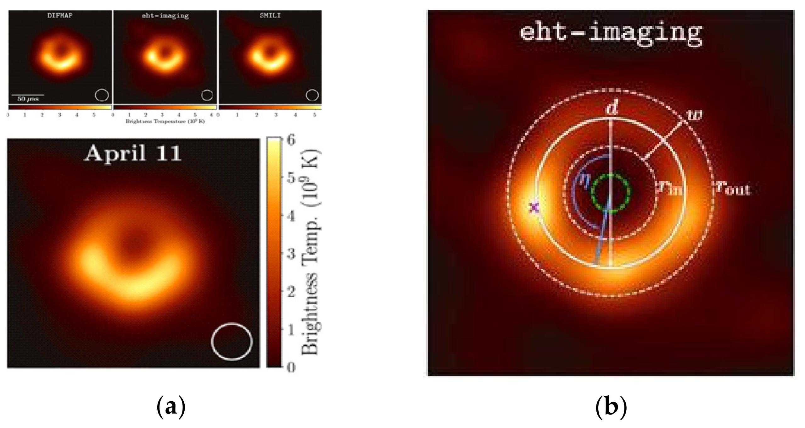
3.2.2. Visualization of the Black Hole Center through the EHT Project

The shadow diameter of M87, which was suspected to be a black hole, was expected to appear at an angle of 19–38 μas from Earth via calculations [9,31]. Scientists expected that the shadow of the black hole could be visualized because each resolution is 20 μas, if measured with a wavelength of 1.3 mm (230 GHz), using very long baseline interferometry (VLBI), with a diameter of approximately equal to the Earth’s diameter (approximately 13,000 km). To develop a telescope with an effective diameter of the scale of the Earth, the EHT project mobilized eight telescopes (i.e., ALMA, APEX, LMT, PV, SMT, JCMT, SMA, and SPT) in six geographical locations (i.e., Chile, Mexico, Spain, Arizona, Hawaii, and Antarctica) [1]. The distances between these telescopes were 0.160–10,700 km, and the maximum angular resolution was 25 μas [9].
The recording of radio waves of a short wavelength (high frequency) requires a very fast data recording speed and vast data storage. In the EHT project, the data were saved at the speed of 64 Gbps. Finally, 15 PB of data were stored in the form of voltage changes of the antenna over time [10]. The PB-level data obtained from each telescope were collected and reduced using three methods (HOPS (Haystack Observatory Processing System. This method was used in calibrating EHT data from early observations) [42], CASA (Common Astronomy Software Applications package. Recently, this method was been frequently used in VLBI) [43], and AIPS (NRAO Astronomical Image Processing System. This method is widely used for radio waves below 86 GHz) [44]) [10].
Because only partial information of the black hole can be obtained through sparsely located telescopes at a very far distance, it is difficult to obtain a single image of the black hole; therefore, it was necessary to find possible images through diverse image processing methods and compare them with each other. The image processing for this purpose was performed in two steps. In Step 1, four teams blindly reconstructed an image of M87 using two methods (CLEAN (This is a reverse modeling method that has been used traditionally in radio telescopes) [39] and RML (Regularized Maximum Likelihood. This is a forward modeling technique that has been developed and used recently) [45]). The images reconstructed by each team had slight differences in ring azimuthal profile, thickness, and brightness; however, they were similar in that the south was brighter and the ring diameter was approximately 40 μas [11]. Hence, in Step 2, the black hole was visualized using three software packages (DIFMAP (A software package based on CLEAN) [46], eht-imaging [47], and SMILI (Eht-imaging and SMILI are open source software libraries specifically developed for EHT based on RML) [48]) based on the two methods used in Step 1. Finally, three images were created using three software packages, and the first image of a black hole was created by averaging these three images, as shown in Figure 5a [11].

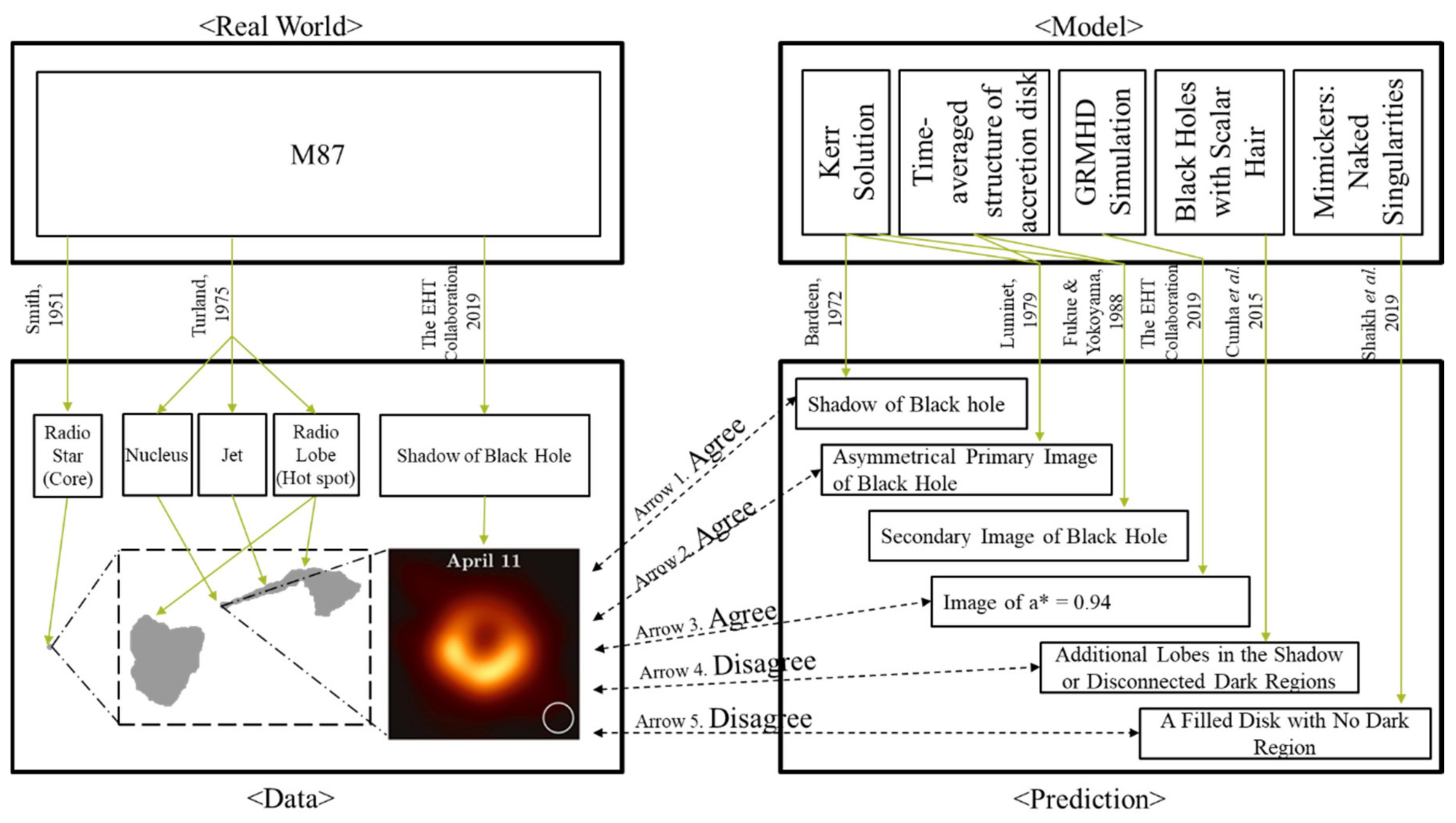
4. Comparison of Visualization between Theoretical Prediction and Actual Observation

According to Giere’s model, data from observations support or modify existing theories or models when they are compared with predictions based on theory. This process is outlined in Giere’s model in Figure 6. The EHT project results illustrate this dynamic process of scientific reasoning. The two-way arrows in Figure 6 indicate how the EHT project results are consistent or inconsistent with the predictions of the existing black hole theories.
Visualization of the black hole periphery through real-world observations before the EHT project did not directly support the theoretical prediction of the black hole shadow; however, through the EHT project, black holes finally became a physical entity that can be researched on and tested, rather than a mathematical concept [1]. Using black hole images, researchers can not only observe the ring with brighter emission in the south, but they can also measure the various features of black holes, such as ring diameter (d), ring width (w), inner and outer diameters of the ring (rin, rout), and orientation angle (η), as shown in Figure 5b [11]. Furthermore, the black hole visualization data obtained through the EHT project enabled the acquisition of additional information by comparing them with theoretically predicted results, and this supported or rejected some theories.
Specifically, the black hole images obtained from the EHT project provided additional information on black holes, based on their comparison with the results of the GRMHD simulation. The GRMHD simulation generated black hole images for various spins (a*) and magnetic fluxes (φ) of black holes. Images similar to the actual observation results could be obtained at a* = −0.94, 0, and 0.94, by comparing the images obtained using the EHT. Among them, the model of a* = −0.94 was rejected because the images were not stable over time, whereas the model of a* = 0 was rejected because it could not explain the conservative lower-limit jet power (Pjet > 1042 erg s−1), which is an existing measurement result [49]. Finally, the model of a* = 0.94 was validated [12].
In addition, diverse data acquired through the black hole images of the EHT project supported some theories and rejected others by evaluating the theories that explained what is at the center of M87. The black hole images were similar to those predicted by the existing theory of general relativity and the Kerr matrix (Arrows 1 and 2 in Figure 6) [26,27]. Therefore, the results of this EHT project still support general relativity and the Kerr solution [1,12]. However, the result of this study rejects various alternative solutions that explain the black hole. First, it rejects general relativity that includes additional fields. Unlike the theory that includes scalar hair, which predicted that there are additional lobes and disconnected dark regions in the shadow of the black hole [28], there was only one dark region in the EHT image (Arrow 4 in Figure 6) [12]. Second, it rejects theories about diverse black hole mimickers. The result of the GRMHD simulation found that only the image with a black hole spin of a* = 0.94 was similar to the EHT image and the superspinar with |a*| > 1 was rejected (Arrow 3 in Figure 6) [12]. Furthermore, naked singularities, which predicted an image without a dark shadow, were rejected (Arrow 5 in Figure 6) [29]. Finally, alternative theories that consist of black hole solutions with classical modifications to general relativity, as well as effects resulting from approaches to quantum gravity [30], were not rejected because they predicted a black hole shadow similar to that of the Kerr solution. These alternative theories could be discussed in the future through further observations of higher frequencies, the degree of polarization, and the variability of the flow of the accretion disk [12].
Currently, VLBI using a shorter wavelength of 0.87 mm is being tested and studies are underway to place additional radio telescopes in spacecraft to increase the effective diameter to larger than the Earth’s radius [1,31,50]. The resulting black hole visualization of higher resolutions could be used to support or reject many alternative theories that have been accepted hitherto and those that will emerge in the future.

5. Educational Significance

In this study, we examined the black hole research process and analyzed the characteristics of the black hole visualization process based on Giere’s model.
Scientists have predicted the images of black holes using various methods based on theories, even when the technical tools for observing black holes were not developed. The development of computer simulation has further improved these methods. For example, additional information on black holes was provided via the GRMHD simulation, and the black hole image for the movie “Interstellar” was created using the DNGR code. However, a higher resolution was required to obtain vivid black hole images through real-world observations, which also required radio telescopes of shorter wavelengths or increased effective diameters. Along with the development of various technologies related to radio telescopes, black hole visualization through observation started from the periphery and has gradually become more mainstream. The EHT project has scientific significance because, for the first time, images of a black hole center were obtained through real-world observations. The information obtained through the black hole images of the EHT project was compared with the characteristics of black holes predicted by existing theories and thereafter used to evaluate the appropriateness of these existing theories. Furthermore, they were combined with other diverse scientific theories, algorithms, and technologies for data transformation, in the process of converting the actual observation data into images.
Therefore, in black hole research, visualizations were obtained neither through simple observations nor through the simple imagination of scientists. Scientists have made boundless efforts toward precise prediction, using theory and visualization, through real-world observational data and their transformation. Diverse scientific theories and technologies are involved in this visualization process. In addition, the results of this visualization ultimately serve to evaluate and develop scientific theories.
It is meaningless for students to view black hole images as mere scientific achievements without understanding the process. Many of the black hole images in current science textbooks used in high schools in South Korea had no descriptions about the image source or the image creation process [51,52,53]. Black hole images and their descriptions in textbooks and educational materials will be revised in the future because it is now possible to use the black hole images of the EHT project. This revision requires the careful attention of science educators. The presentation of black hole images in science education is important because understanding the scientific process is as important as learning scientific concepts. Black hole images can help students understand not only the appearance and structure of black holes but also the roles and significance of visualization in scientific research. This requires an explanation regarding the creation of the black hole images and their sources. Moreover, an explanation is also required on whether the images are the results of theoretical simulations, simple imaginary drawings, or images based on observation, as well as their creation process.
Students should understand the following if they not only use the black hole images of the EHT project as the results of science but to also improve their understanding of the scientific process:
  • The images obtained via the EHT project are not the only images of the black holes. For a substantially long period of time, scientists have predicted and studied black hole images based on scientific theories. In science, simulation based on theories is as important as actual observation.
  • The images obtained via the EHT project required a complex data transformation process. They are the result of creating whole images from partial images, through various comparisons and evaluations, in which many theories are involved. These images were not obtained from direct visual observations using telescopes with high magnifications.
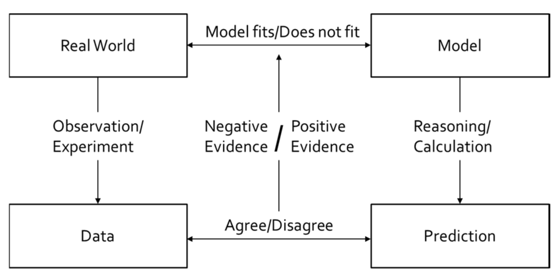
  • The images obtained via the EHT project are compared with the characteristics and images of black holes predicted using theories and are used to evaluate the appropriateness of the existing theories on black holes. The results of real-world observations influence the creation and modification of theories.
  • The images obtained via the EHT project are not the final images of black holes; rather, they enable various subsequent studies on black holes. The black hole images obtained via the EHT project are the products of scientific research and a stepping stone that enables further research.
As visualization and visual representation are critical in scientists’ research processes, visual representation is also critical and essential for science education [54]. Most scientific knowledge and principles, including structures and appearances of animals and plants, the principle of shadows, motor mechanism, and structures of atoms and molecules, are difficult to explain or understand without visual representations. In the movie “Interstellar,” visualizations for the public showed slightly different characteristics to those for scientists. Some important features of the black hole (e.g., asymmetry due to the Doppler effect) were removed, and the black hole was visualized to provide a familiar image to the nonspecialist. Learners are in the middle of the general public and scientists. It is therefore necessary to discuss what properties could be removed and kept in the visualization for students. Visual representations can not only be used to understand and memorize scientific concepts but to also understand the nature of science and the characteristics of scientific reasoning. In particular, as the direct perception of black holes by humans is difficult, understanding the efforts that scientists have made and the methods they seek to employ to visualize black holes, as well as understanding the development of science as a consequence of such research, will help foster true scientific literacy.

Author Contributions

Conceptualization, H.-G.Y.; Formal analysis, J.P. and I.L.; Funding acquisition, H.-G.Y.; Investigation, J.P. and I.L.; Methodology, J.P. and I.L.; Project administration, H.-G.Y.; Resources, J.P. and I.L.; Supervision, H.-G.Y.; Validation, H.-G.Y.; Visualization, J.P.; Writing—original draft, H.-G.Y. and J.P.; Writing—review & editing, H.-G.Y. and I.L. All authors have read and agreed to the published version of the manuscript.

Funding

This research was funded by the National Research Foundation of Korea (NRF) grant funded by the Korea government (MIST: Ministry of Science and ICT), No. 2019R1F1A1040353.

Conflicts of Interest

The authors declare no conflicts of interest.

References

  1. EHT Collaboration. First M87 Event Horizon Telescope results. I. The shadow of the supermassive black hole. Astrophys. J. Lett. 2019, 875, L1. [Google Scholar] [CrossRef]
  2. Giere, R.N.; Bickle, J.; Mauldi, R.F. Understanding Scientific Reasoning; Thomson Wadsworth: Melbourne, VIC, Australia, 2006. [Google Scholar]
  3. Thorne, K. Black Holes & Time Warps: Einstein’s Outrageous Legacy; WW Norton & Company: New York, NY, USA, 1995. [Google Scholar]
  4. Park, S. Einstein and Hawking’s Black Hole; Whistler: Seoul, Korea, 2005. [Google Scholar]
  5. Woo, J. Prof. Woo’s Black Hole Lecture; Gimm-Young Publishers, Inc.: Seoul, Korea, 2019. [Google Scholar]
  6. Luminet, J.P. An illustrated history of black hole imaging: Personal recollections (1972–2002). arXiv 2019, arXiv:1902.11196. [Google Scholar]
  7. Ramakrishnan, V. Seeing is believing. Resonance 2019, 24, 529–534. [Google Scholar] [CrossRef]
  8. Falcke, H. Imaging black holes: Past, present and future. J. Phys. Conf. Ser. 2017, 942, 012001. [Google Scholar] [CrossRef]
  9. EHT Collaboration. First M87 Event Horizon Telescope results. II. Array and instrumentation. Astrophys. J. Lett. 2019, 875, L2. [Google Scholar] [CrossRef]
  10. EHT Collaboration. First M87 Event Horizon Telescope results. III. Data processing and calibration. Astrophys. J. Lett. 2019, 875, L3. [Google Scholar] [CrossRef]
  11. EHT Collaboration. First M87 Event Horizon Telescope results. IV. Imaging the central supermassive black hole. Astrophys. J. Lett. 2019, 875, L4. [Google Scholar] [CrossRef]
  12. EHT Collaboration. First M87 Event Horizon Telescope results. V. Physical origin of the asymmetric ring. Astrophys. J. Lett. 2019, 875, L5. [Google Scholar] [CrossRef]
  13. EHT Collaboration. First M87 Event Horizon Telescope results. VI. The shadow and mass of the central black hole. Astrophys. J. Lett. 2019, 875, L6. [Google Scholar] [CrossRef]
  14. Schwarzschild, K. Über das Gravitationsfeld eines massenpunktes nach der Einsteinschen theorie. Sitz. Deut. Akad. Wiss. Math. Phys. Berlin 1916, 18, 189–196. [Google Scholar]
  15. Kerr, R.P. Gravitational field of a spinning mass as an example of algebraically special metrics. Phys. Rev. Lett. 1963, 11, 237. [Google Scholar] [CrossRef]
  16. Page, D.N.; Thorne, K.S. Disk-accretion onto a black hole. Time-averaged structure of accretion disk. Astrophys. J. 1974, 191, 499–506. [Google Scholar] [CrossRef]
  17. Fukue, J.; Yokoyama, T. Color photographs of an accretion disk around a black hole. Publ. Astron. Soc. Japan 1988, 40, 15–24. [Google Scholar]
  18. Bardeen, J.M. Timelike and null geodesics in the Kerr metric. In Black Holes (Les Astres Occlus); Dewitt, C., Dewitt, B.S., Eds.; Gordon and Breach: New York, NY, USA, 1973. [Google Scholar]
  19. Müller, T.; Weiskopf, D. Distortion of the stellar sky by a Schwarzschild black hole. Am. J. Phys. 2010, 78, 204–214. [Google Scholar] [CrossRef]
  20. Riazuelo, A. Seeing relativity-I: Ray tracing in a Schwarzschild metric to explore the maximal analytic extension of the metric and making a proper rendering of the stars. Int. J. Mod. Phys. D 2019, 28, 1950042. [Google Scholar] [CrossRef]
  21. Luminet, J.P. Black Holes; Cambridge University Press: Cambridge, UK, 1992. [Google Scholar]
  22. Cunningham, C.T.; Bardeen, J.M. The optical appearance of a star orbiting an extreme Kerr black hole. Astrophys. J. 1973, 183, 237–264. [Google Scholar] [CrossRef]
  23. Luminet, J.-P. Image of a spherical black hole with thin accretion disk Astron. Astron. Astrophys. 1979, 75, 228–235. [Google Scholar]
  24. Viergutz, S.U. Image generation in Kerr geometry. I. Analytical investigations on the stationary emitter-observer problem. Astron. Astrophys. 1993, 272, 355–377. [Google Scholar]
  25. James, O.; Von Tunzelmann, E.; Franklin, P.; Thorne, K.S. Gravitational lensing by spinning black holes in astrophysics, and in the movie Interstellar. Class. Quantum Gravity 2015, 32, 065001. [Google Scholar] [CrossRef]
  26. Dexter, J.; McKinney, J.C.; Agol, E. The size of the jet launching region in M87. Mon. Not. R. Astron. Soc. 2012, 421, 1517–1528. [Google Scholar] [CrossRef] [Green Version]
  27. Mościbrodzka, M.; Falcke, H.; Shiokawa, H. General relativistic magnetohydrodynamical simulations of the jet in M 87. Astron. Astrophys. 2016, 586, A38. [Google Scholar] [CrossRef]
  28. Cunha, P.V.P.; Herdeiro, C.A.R.; Radu, E.; Rúnarsson, H.F. Shadows of Kerr black holes with scalar hair. Phys. Rev. Lett. 2015, 115, 211102. [Google Scholar] [CrossRef] [PubMed] [Green Version]
  29. Shaikh, R.; Kocherlakota, P.; Narayan, R.; Joshi, P.S. Shadows of spherically symmetric black holes and naked singularities. Mon. Not. R. Astron. Soc. 2019, 482, 52–64. [Google Scholar] [CrossRef]
  30. Giddings, S.B.; Psaltis, D. Event horizon telescope observations as probes for quantum structure of astrophysical black holes. Phys. Rev. D 2018, 97, 084035. [Google Scholar] [CrossRef] [Green Version]
  31. Johannsen, T.; Psaltis, D.; Gillessen, S.; Marrone, D.P.; Özel, F.; Doeleman, S.S.; Fish, V.L. Masses of nearby supermassive black holes with very long baseline interferometry. Astrophys. J. 2012, 758, 30. [Google Scholar] [CrossRef] [Green Version]
  32. Messier, C. Catalogue des Nébuleuses et des Amas d’Étoiles (Catalog of Nebulae and Star Clusters); L’Imprimerie Royale: Paris, France, 1781. [Google Scholar]
  33. Curtis, H.D. Descriptions of 762 nebulae and clusters photographed with the crossley reflector. Pub. Lick Obs. 1918, 13, 9–42. [Google Scholar]
  34. Smith, F.G. An accurate determination of the positions of four radio stars. Nature 1951, 168, 555. [Google Scholar] [CrossRef]
  35. Macdonald, G.H.; Kenderdine, S.; Neville, A.C. Observations of the structure of radio sources in the 3C catalogue—I. Mon. Not. R. Astron. Soc. 1968, 138, 259–311. [Google Scholar] [CrossRef] [Green Version]
  36. Hogg, D.E.; MacDonald, G.H.; Conway, R.G.; Wade, C.M. Synthesis of brightness distribution in radio sources. Astron. J. 1969, 74, 1206–1213. [Google Scholar] [CrossRef]
  37. Turland, B.D. Observations of M87 at 5 GHz with the 5-km telescope. Mon. Not. R. Astron. Soc. 1975, 170, 281–294. [Google Scholar] [CrossRef] [Green Version]
  38. Hines, D.C.; Owen, F.N.; Eilek, J.A. Filaments in the radio lobes of M87. Astrophys. J. 1989, 347, 713–726. [Google Scholar] [CrossRef]
  39. Högbom, J.A. Aperture synthesis with a non-regular distribution of interferometer baselines. Astron. Astrophys. Suppl. Ser. 1974, 15, 417–426. [Google Scholar]
  40. Clark, B.G. An efficient implementation of the algorithm ‘CLEAN’. Astron. Astrophys. 1980, 89, 377–878. [Google Scholar]
  41. Gull, S.F.; Northover, K.J.E. Bubble model of extragalactic radio sources. Nature 1973, 244, 80–83. [Google Scholar] [CrossRef]
  42. Whitney, A.R.; Cappallo, R.; Aldrich, W.; Anderson, B.; Bos, A.; Casse, J.; Goodman, J.; Parsley, S.; Pogrebenko, S.; Schilizzi, R.; et al. Mark 4 VLBI correlator: Architecture and algorithms. Radio Sci. 2004, 39, 1–24. [Google Scholar] [CrossRef]
  43. McMullin, J.P.; Waters, B.; Schiebel, D.; Young, W.; Golap, K. CASA architecture and applications. ASP Conf. Ser. 2007, 376, 127–130. [Google Scholar]
  44. Greisen, E.W. The FITS interferometry data interchange convention—Revised. AIPS Memo Ser. 2016, 114, 1–59. [Google Scholar]
  45. Thiébaut, É. Principles of image reconstruction in interferometry. EAS Publ. Ser. 2013, 59, 157–187. [Google Scholar] [CrossRef]
  46. Shepherd, M. Difmap: Synthesis Imaging of Visibility Data; ascl: 1103.001. ASCL: Leicester, UK, 2011. Available online: http://ascl.net/1103.001 (accessed on 11 April 2020).
  47. Chael, A.; Bouman, K.; Johnson, M.; Wielgus, M.; Blackburn, L.; Chan, C.; Farah, J.R.; Palumbo, D.; Pesce, D. eht-imaging: v1.1.0: Imaging Interferometric Data with Regularized Maximum Likelihood. Available online: https://zenodo.org/record/2614016#.XspLf8ARVPY (accessed on 24 May 2020).
  48. Akiyama, K.; Tazaki, F.; Moriyama, K.; Cho, I.; Ikeda, S.; Sasada, M.; Okino, H.; Honma, M. SMILI: Sparse Modeling Imaging Library for Interferometry. Available online: https://zenodo.org/record/2616725#.XsuzR2gzaUk (accessed on 24 May 2020).
  49. Young, A.J.; Wilson, A.S.; Mundell, C.G. Chandra imaging of the X-ray core of the Virgo cluster. Astrophys. J. 2002, 579, 560–570. [Google Scholar] [CrossRef] [Green Version]
  50. Roelofs, F.; Falcke, H.; Brinkerink, C.; Mościbrodzka, M.; Gurvits, L.I.; Martin-Neira, M.; Kudriashov, V.; Klein-Wolt, M.; Tilanus, R.; Kramer, M.; et al. Simulations of imaging the event horizon of Sagittarius A* from space. Astron. Astrophys. 2019, 625, A124. [Google Scholar] [CrossRef] [Green Version]
  51. Kim, Y.M.; Kim, I.G.; Kim, J.K.; Kim, J.B.; Park, B.Y.; Jung, H.J.; Hanh, I. Physics II; Kyohaksa: Seoul, Korea, 2018. [Google Scholar]
  52. Kim, S.W.; Shin, S.; Oh, K.; Lee, S.K.; Lee, Y.; Jang, J. Physics II; Jihaksa: Seoul, Korea, 2018. [Google Scholar]
  53. Lee, K.Y.; Kim, H.S.; Park, J.; Lee, S.M.; Jeong, J.H.; Choi, Y. Earth Science I; Visang: Seoul, Korea, 2018. [Google Scholar]
  54. Lemke, J. Multiplying meaning: Visual and verbal semiotics. In Scientific Text Reading Science: Critical and Functional Perspectives on Discourses of Science; Martin, J.R., Veel, R., Eds.; Routledge: London, UK, 1998. [Google Scholar]
Figure 1. Scientific reasoning model (redrawn from [2]).
Universe 06 00070 g001
Figure 2. Schematic of the black hole visualization.
Universe 06 00070 g002
Figure 3. Black hole images made with a theory-based prediction: (a) First black hole image [23] (Luminet, J.-P, A&A, 75, 235, 1979, reproduced with permission © ESO); (b) Black hole image in the film Interstellar [25]. The upper part of the figure represents the primary image of the disk and the lower part shows the secondary image.
Universe 06 00070 g003
Figure 4. Images of the periphery of a black hole based on measurements: (a) M87 visualized with contour lines (from Figure 1, observations of M87 at 5 GHz with the 5 km telescope, Turland, D. B., Mon. Not. R. Astron. Soc., 170) [37]; (b) Image of the total intensity of M87 (from Figure 3, Hines, D.C.; Owen, F.N.; Eilek, J.A. Filaments in the radio lobes of M87. Astrophys. J. 1989, 347, 713-726. © AAS. Reproduced with permission) [38].
Universe 06 00070 g004
Figure 5. The first image of a black hole [11]: (a) Image of a black hole, created by averaging these three images; (b) Measurement of the various features of the black hole.
Universe 06 00070 g005
Figure 6. Overview of studies regarding black hole visualization analyzed by using Giere’s model.
Universe 06 00070 g006

