Abstract
The model of a multiverse is advanced, which endows subuniverses like ours with space and time and imparts to their matter all information about the physical laws. It expands driven by dark energy (DE), which is felt in our Universe (U) by mass input and expansion–acceleration. This dark multiverse (DM) owes its origin to a creatio ex nihilo, described in previous work by a tunneling process in quasi-classical approximation. Here, this origin is treated again in the context of quantum gravity (QG) by solving a Wheeler de Witt (WdW) equation. Different than usual, the minisuperspace employed is not spanned by the expansion parameter a but by the volume . This not only modifies the WdW-equation, but also probabilities and solution properties. A “soft entry” can serve the same purpose as a tunneling process. Sections of solutions are identified, which show qualitative features of a volume-quantisation, albeit without a stringent quantitative definition. A timeless, spatially four-dimensional primordial state is also treated, modifying a state proposed by Hartle and Hawking (HH). For the later classical evolution, elaborated in earlier papers, a wave function is calculated and linked to the solutions for the quantum regime (QR). It is interpreted to mean that the expansion of the DM proceeds in submicroscopic leaps. Further results are also derived for the classical solutions.
1. Introduction
The multiverse conception is currently in a state which is comparable to that of black holes before the proof of their existence. Because one does not know for sure if something like a multiverse exists, and since all the more nothing is known about its properties, the occupation with multiverses has the touch of the exotic. In addition, it is not foreseeable that one comes to solid conclusions about their existence and characteristics as fast as with black holes. It is therefore not surprising that there are very different concepts for them. It is certainly advantageous, if a concept sticks to proven equations: it has often turned out that previously unknown phenomena are actually realized in nature, if they are in harmony with approved physics. In addition, it would speak for a specific concept if detectable influences on U would result from it. However, it cannot be ruled out that a concept, based on modified basic equations, will finally prevail. If some day a particular concept comes out on top, the others become more or less obsolete, which could of course also happen to the current concept. However, that does not necessarily mean that the others were completely worthless because they could have paved the way for the ultimate winner.
The present concept was initiated in Ref. [1], refined in Ref. [2] and is further developed in this paper. The most important results of the earlier work are briefly summarized in Section 2. Section 3 deals with two scenarios for the origin of the DM, the first with a tunneling process as proposed by Vilenkin [3,4] and Linde [5] (VL), and the second with a modification of a timeless primordial state proposed by Hartle and Hawking [6]. Both scenarios are dealt with by using two methods, 1. relatively short with a quasi-classical, approximate treatment of the QR, and 2. much more detailed in the context of QG by solving an unusual WdW-equation, which we consider appropriate and deduce in the Appendix. Furthermore, an equation for the classical regime (CR) is derived, whose solution is smoothly connected to that for the QR and interpreted in a special way. In doing so, we encounter a solution that represents an alternative to the tunneling solution and can be called a “soft entry”. In Section 4.1, we critically reflect on the basic idea of our DM-concept, the storage and transmission of information about the laws of physics. In this context, we point to difficulties arising from loop theory of QG (LQG) and suggest ways in which they may be overcome. The identification of solution sections exhibiting properties of a spatial volume quantisation provides this subsection with a particular significance. In Section 5, properties of the classic solution are elaborated, which were only hinted at or not dealt with in Ref. [2]. At first, the conditions are calculated, which, allowing for primordial matter, enable an (unstable) equilibrium between this and the DE at the beginning of the DM-expansion.
Then, the minimal the age of the DM is calculated, which is compatible with the maximum curvature allowed by corresponding measurements in U. It is also clarified how it comes about that the irreversible solution of the cosmological equations with a friction term in the equation for the expansion acceleration, , solves as well the reversible equations for a scalar field driven expansion. Finally, it is investigated how the DM-expansion behaves in comparison to the expansion of U.
For the readers’ convenience, all abbreviations are listed before Appendix A.
2. Summary of Previous Work on the DM-Concept
Essence and determination of the considered DM are that the latter provides space and time for subuniverses with ours among them, i.e., the latter arise in an already prefabricated space. Thus, it was not generated along with them but long before. Thus far, we assumed that it originated at a finite time in the past by a creation from nothing, emerging continuously from nothingness through quantum mechanical tunneling. For this, it must be a closed and expanding multiverse of positive curvature, if topologically more complex situations (three-torus) are excluded, and its expansion must start at zero velocity immediately after the tunneling. The maximum spatial curvature that would be compatible with relevant measurements of negative result is so small that the space, in which U lives, extends far beyond its particle horizon. As a consequence, large areas exist outside that are causally not connected with the interior, are thus structurally quite different, and can be considered as parts of a multiverse embracing U.
The ingredient forming the backbone of the DM or the space-time spanned by it, respectively, is assumed to be dark energy (DE). It is no additional extra, but the medium which is generating space and time. Subuniverses like ours are assumed to originate from fluctuations of independent inflation fields. Since the DE of the DM also fills U, it can be considered as a fingerprint of the DM on U. It causes not only a continuously accelerated expansion of the DM but is also responsible for the accelerated expansion presently observed in U, if its mass density is properly adjusted. If, as in inflation theories, its initial value is chosen close to the Planck density, then must decay by a factor of about so it can be identified with the DE observed in U. The decay factor agrees approximately with the factor, by which the presently observed mass density of the cosmological constant differs from the value predicted by elementary particle theory. This suggested the assumption of a mechanism, by which, in the course of the increasing expansion of the DM, the effect of a huge and unchangeable cosmological constant is continuously reduced down to its present much lower efficiency. It turned out that this mechanism can be intimately linked to a proposed solution for another, so far largely ignored conundrum of physics, namely the question of how it comes about that in each point of space-time the physical laws are obeyed.
For this purpose, going far beyond what was set out above, we assumed that the space-time of the DM is of a very special kind in that it is encoded with all the information about the physical laws, to which all material components occurring in the subuniverses must obey. This could be achieved in a geometric way, as is the case with the laws of gravitation according to the general theory of relativity, or with the laws of electrodynamics, using an additional spatial dimension as in the Kaluza–Klein theory. Alternatively, the physical laws could as well be stored in subatomic structures of a granular space-time in a similar way as the laws of biological growth are encoded in the DNA. According to our former assumptions, the information about all physical laws, and the physical agents to whom they relate, is transmitted through the creational tunneling process to the subsequent initial state of the DM. This means that the primordial nothingness is understood as a state of pure information without space and time.
As stated above, we assume that keeps its large initial value during the whole evolution of the DM. Without reduction it would cause an extremely accelerated expansion. The space added by this must be equipped with all information listed above via transfer from already existing space. This will take time that is not available, if the spatial expansion proceeds too fast. Therefore, we assumed that this transfer impedes the spatial expansion, and that this can be cumulatively represented by a friction term in the cosmological equations. Without it, the Friedman–Lemaître (FL) equation would be with the immediate consequence . Introducing a linear friction term, the latter equation becomes
where is a constant. Multiplication with and integration with respect to t yields
The integration constant was chosen such that, at , the time immediately after the tunneling process, the DM starts with and , where
( and with = Planck length, = Planck density), and evolves according to the usual FL-Equation (2). It is therefore possible to say that our model leads to solutions of the standard theory which are only re-interpreted in an unusual way. In Ref. [2], it was shown that even the cosmological equations for a scalar field , driven by a potential , are satisfied. As a result, the interaction of the huge cosmological constant with energy density and the friction force of Equation (1) has exactly the same effect as a dark energy (exerting an anti-gravitational force and providing mass in our universe), which is represented by a scalar field with energy density , and is therefore also referred to as DE. Its origin is inseparably linked to the emergence of space-time because, according to the above, the latter is generated by it. Because of the associated information about properties like mass or charge, in principle, particles should also be incorporated in the FL-equation at least in the form of a cumulative mass density. Since this would not disclose anything new as compared to the results of Ref [1], as in Ref [2], this is relinquished here.
In the dimensionless quantities,
( = Planck time), Equations (1) and (2) become1
and
The solution of the last equation for the initial conditions and at is
Employing the Wick rotation for , Equation (6) is converted into
For and plus at , the solution , shown in Figure 1, is obtained. Since and are both extremely small,
is an excellent approximation. Equation (6) is satisfied by calculating from it the mass density
Inserting in it solution (9), using Equation (4) and the last of Equations (3), and cutting out , we obtain for the present state by solving for
where is the value of the DE-density measured at present in U, and (with present age of U) is the condition that allows the neglect of according to Ref. [2]. Because is so small, holds according to Equation (10), and the volume is given by according to Equation (A10) of the Appendix. The total energy of M is therefore , so it grows with increasing expansion . Consequently, the friction force does not, as usual, convert potential energy into heat; instead, it only slows down the energy increase of M and, simultaneously, the decrease of (negative) gravitational energy.
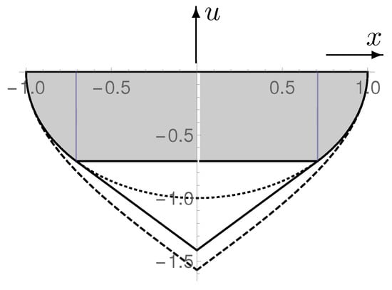
Figure 1.
Approximate solutions for the QR, discussed from the bottom up. 1. dashed curve: , 2. full curve: solution (13) continued by straight lines, 3. dotted curve: semicircle, 4. curve with gray filling: HH-like solution.
Annotation: We consider the case only in Section 4.1, everywhere else we assume .
3. Two Scenarios for the Origin of the Dark Multiverse
In Refs. [1,2], it was assumed that the DM comes about by a creation from nothing, conveyed by a quantum mechanical tunneling process as introduced into cosmology by Vilenkin [3,4] and Linde [5]. At about the same time, Hartle and Hawking presented a quite different proposal, according to which the primordial condition of the universe is a timeless quantum state in four spatial dimensions on equal footing, filling essentially a 4D-sphere. The VL-approach employs four spatial coordinates as well; however, one of them comes out by a Wick rotation of the time, a mathematical tool, by which the effectively time-dependent tunneling process is described in a particularly easy, albeit approximate manner. In the HH-approach, on the other hand, the positively curved space is truly four-dimensional; due to symmetry requirements (no boundary condition), no point is distinguished from the others, which in any way could be interpreted as a starting point. Nevertheless, time is still implicitly contained in that the wave function of the timeless state is linked to a three-dimensional probability density and depends on the metric coefficients of a 3D-space, while matter fields involve a 3D-mass-density. No simple approximation of the quantum behavior is possible as in the VL-approach, rather a true quantum theory of the gravitational field must be invoked. For this purpose, the WdW-equation is chosen, according to which the states of the multiverse are generally timeless.
In this paper, two separate approaches are undertaken, the first modifying the VL-approach, and the second the HH-approach.
3.1. Quasiclassical Approximation of the Quantum Regime
- Creation from nothing through tunneling. It is interesting to look into the question of whether a tunneling solution of Equation (8) is also possible when , as in the HH-approach, forms a semicircle (page 86 of Ref. [7]) so that no point is distinguished. Accordingly, we demand the validity of the equationand determine from Equation (8) in such a way that Equation (12) is satisfied. From the latter follows . Inserting this in Equation (8), eliminating u by use of Equation (12), and resolving with respect to yieldsThis treatment of the QR is an approximation which is getting worse the deeper one gets into it. In that sense, the negative values of the density may perhaps not be taken seriously. However, for , a singularity appears that is just what should be avoided in a quantum treatment.There are two ways to get out of this situation with a viable solution.1. the solution (13), yielding in the range , is continued into the range by a straight line with the slope following from Equation (8) for .2. The solution (13) is cut off at .Both possibilities are shown in Figure 1. The truncated HH-like solution, supplemented by two straight lines, has a peak which constitutes a distinguished point and must therefore be regarded as a tunneling solution of the VL-type. It represents an alternative to the solution (45) of Ref. [2], or , but does not comply with the HH-concept.
- HH-like primordial state. In the case of the solution cut off at with , the situation changes. If the two end points are connected by a horizontal straight line and the resulting corners rounded, one arrives at a solution, whose boundary, although not having a constant curvature, does not contain any point which could be interpreted as a temporal beginning. Although this solution results from the effort to construct a VL-like tunneling solution, it makes sense to accept it as a solution compatible with the HH-intention, so that the fourth spatial coordinate (which resulted from time by a Wick Rotation) is on equal footing to the others. It is obvious that the treatment of this model with the WdW-equation in the context of QG is much more appropriate because of its time independence.
3.2. Employing Quantum Gravity with Use of a Wheeler-De Witt Equation
In this section, the solution of the WdW-equation [8,9], applied to a properly chosen minisuperspace, is used to investigate the tunneling process considered in Ref. [2] (and ending up in a modification of the latter), and a modified HH-concept. Despite the 50 years that have passed since the introduction of this equation, and despite the many papers and book contributions in which it was treated, it is still not as straightforward as in ordinary quantum mechanics to find the right solution for a given concept and to interpret it appropriately (see e.g., [10], quoted in pages 206–207 of Ref. [11], or page 135 of Ref. [12]). This is partly because there are two types of probability interpretation, either by transition probabilities or by the square of the wave function. In addition, problems arise with respect to the Hermiteness of operators, setting proper boundary conditions, and the role of time. Considerable effort was made to find analytic solutions to the WdW-equation (see e.g., [13]) and study such conditions with them.
The ambition of this paper goes in a different direction. We want to use the square of the wave function for calculating probabilities. However, regarding its normalization and the associated probability interpretation, we try a way that deviates from the usual. In doing so, we find it useful to base the WdW-equation on a different minisuperspace for the following reason: in several places, the three-dimensionality of space enters the relevant WdW-equation in a decisive way. This can be seen in its derivation, which is therefore carried out in the Appendix A with reference to the critical points. Furthermore, densities contained in it like relate to three dimensions. Finally, the three-dimensionality is also reflected in solutions. On the one hand, the wave function for the CR depends on , if it is calculated in the usual way (see item 3 in Section 3.2.1). On the other hand, its square, the probability density, decreases over time instead of increasing as expected. All of this has prompted us to choose instead of a as the variable spanning the minisuperspace. This leads not only to more plausible probability densities, but also to a modified WdW-equation.
3.2.1. Creation from Nothing
- Solution in the QR. In finding the right solution for a creation from nothing, we restrict ourselves to the option 2, for which we must solve Equation (A9) (with ),According to pages 203–206 of Ref. [11], a solution is considered the best, for which is largest at and decreases fast with increasing x because it roughly corresponds to the tunneling through the potential barrier given by the factor ∼ near in Equation (A8). We take the position that probability statements make sense only within an already existing multiverse, while conclusions based on such statements about the start of the tunneling are external, that is, they come from nowhere and must be regarded as meaningless. In the selection of a solution for an equivalent process, being suggested as a viable alternative on page 204 of Ref. [11] with reference to Ref. [10], we rely entirely on the probability interpretation of and choose so that with increasing v its square permanently increases. The solution shown in Figure 2 has this property; in the place where it is linked with the wave function for the CR, it satisfies the further constraint , which is explained further down. In the next paragraph, another argument is developed which supports our selection. Although derived with the goal of a tunneling process, this solution has nothing in common with the latter and therefore should be named differently, e.g., “soft entry”. Equation (14) has, of course, also a genuine tunneling solution, which can be treated in exactly the same way as our “soft entry” solution.
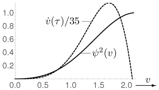
- Interpretation. Contributions to the literature on QG such as [14,15,16] give the impression that too little information is available for the assignment and interpretation of the WdW-equation. In Ref. [16], the interesting suggestion is made to use the de Broglie–Bohm interpretation for this purpose. According to this, from the representation of the wave function, particle trajectories satisfying are derived. Unfortunately, this is not possible in our case because the solutions of Equation (14) are real whence . Therefore, we develop an alternative, which, like the de Broglie–Bohm approach, leaves quantum mechanics completely unchanged and concerns only its interpretation. Under application to the solutions of Equation (14), it consists essentially in reversing the step that leads from the classical to the quantum-mechanical description. Specifically, for the spatial density of the quantum mechanical momentum, we make the ansatz( is obtained from Equations (A2)–(A4)) by which it is identified with the classical momentum. The multiplication of the left side by i constitutes the return to classical values and can be interpreted as reverse Wick rotation. With Equations (4), , , and going over to dimensionless quantities, and resolving with respect to , the last equation becomesThis means that the DM moves to larger values of until it terminates the entry process, if everywhere . The velocity and , up to a normalization factor the probability density of our “soft entry” solution, are depicted in Figure 2. From that, it becomes particularly clear that our solution is suitable for describing a creation from nothing. Regarding the dynamics, one could even say, at least for this solution that in the QR the role of time is taken over by the probability density .
- Wave function of the the CR. We want to connect the wave function of the QR with that of the CR and have to determine the latter. For this, it is advantageous to use the interpretation of the classical solution based on Equations (5) and (6) with a friction term because then the minisuperspace contains only the one variable v. Furthermore, we can use the fact that we already know the classical solution (9), which satisfies the equationWe first consider the quantisation of the latter in the minisuperspace spanned by a or x resp. This can be done in the same way as in the derivation of Equation (A7). With , Equation (17) becomes . The equation corresponding to Equation (A2) is obtained by setting , and . With this, one can go directly to Equation (A6) and from there to dimensionless quantities, ending up at the WdW-equationIts general solution iswhere are Bessel functions, and a and b are integration constants. As mentioned in the introduction to Section 3.2, the solution depends on the volume . Furthermore, for , the envelope of the Bessel functions is whence, due to the factor in front of , the envelope of decays with u as . This solution would actually lead the DM-expansion to ever smaller probabilities, so absolutely not what one would reasonably expect.The situation turns for the better, if we employ the minisuperspace spanned by v. The corresponding WdW-equation can be easily deduced from Equation (18) by replacing in it by according to Equation (A10). The resulting equation isand has the solutionwhere is an integration constant. This solution must be continuously and with continuous derivative be connected to the solution for the QR, that of Equation (14). For the latter as well as for Equation (20), it holds that together with also is a solution, where C is a freely selectable constant. This allows us to freely set the value of one of the two solutions at the junction and to continuously join the other. Due to the extremely small value of , the derivative of the solution (21) for the CR is essentially equal to zero for all v. It follows that the derivative of the solution for the QR must be virtually zero at the junction. For the sake of simplicity, we therefore demand that the derivative of both solutions is exactly zero at the junction. With the boundary condition for the QR-solution at the border to the CR, it follows from Equation (16) that there also and thus must apply. Thus, QG requires the same boundary condition as the quasi-classical approximation.Figure 3 shows the solutions thus obtained. The joining point is or and not as in Section 3.1. This is due to the requirement and the fact that Equation (14) does not allow a solution with and . The classical solution (21) is entered twice in the figure, once over (horizontal straight line), and once over (dashed curve).
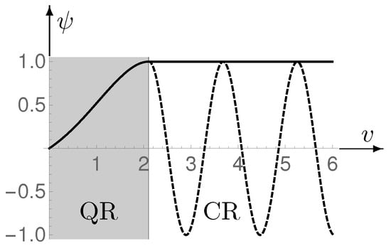 Figure 3. The full curve is a joint representation of the “soft entry” solution for the QR (gray filling) and for the CR. The dashed curve shows once again, but highly compressed in the horizontal direction in order to visualize the oscillations.
 - Normalization of and corresponding probabilities. The freely selectable factor C in the solutions of Equations (14) and (20) allows a particularly simple fulfillment of the normalization condition (A11), for which onlymust be chosen. The normalized solution is then . This does not only apply to the solution for the QR, but also to combined solutions for the QR and the CR. For comparing states that have been traversed up to a certain time (corresponding volume ), it appears reasonable to extend the normalization range from up to . Over time, the upper boundary becomes larger and larger, with the result that the probability density of fixed and duly normalized intermediate states becomes ever smaller. Therefore, it is obviously useless to compare intermediate states of different normalization. In other words, it only makes sense to compare states with the same normalization, which amounts to determining the ratio of their probabilities. However, this is just as well obtained from a wave function without normalization, which is valid for the entire range. (This is the reason why our figures are not based on normalized wave functions.)For interpreting the dynamics of the system described by the wave function (21), the probability density can not be used as in the case of the “soft entry” solution. The reason is that it has many local maxima, and the system would remain with one of them, once it has reached it. This problem can be solved by considering the set of values between two successive zeros as a single quantum state of the classical system. This range has the size following from or and corresponds to the x-range orwhere Bohr radius. Regarding the dynamics, we assume that the system jumps from one state to the next in leaps of the length . In this interpretation, up to an uninteresting factor, the probability density of the various system states is given by the average of the local density over a half period, that is, byWith our solution, the probability of the different states does not decrease as with the solution (19) based on the usual minisuperspace. However, it does not increase as desired either. This can, however, be improved by taking advantage of the fact that the classical dynamic is an evolution in time, and by relating the probability density not to volume but to time (using instead of ). Settingfor we employ the classical solution: from and use of Equation (9), we get and finallywhere v does the jumps of height described above. Plotted above v, thus follows a staircase-like curve of the slope . Once again, the incremental probability of the individual quantum states can be considered as a substitute for time.
3.2.2. Modified HH-Approach
- Depictive model. In this section, we investigate an alternative to the HH-approach which differs comparatively more from the latter than the approach in Section 3.1. We now assume that the timeless primordial state is a 4D-sphere of radius in a 4D-space (coordinates ) of constant positive curvature, uniformly filled with DE of the 3D-density . It can be represented by the surfaceof a 5D-sphere in a Euclidean 5D-space. Assuming that the 3D-subspace spanned by is homogeneous and isotropic, its metric belongs to the class of metrics with line elementwhere and . For both and , a 3D-space of the same metric is transversed, so one can say that, for given a, two identical homogeneous, isotropic and closed 3D-spaces of Volume exist. Due to the factor , not present in the representation (24) of the surface of the initial 5D-sphere, the metric of its homogeneous and isotropic 3D-sub-spaces is a subclass of the metrics of Equation (24). We must therefore find out which restrictions result for the expansion parameter a. According to Equation (24), for , from which it follows that and . A maximum value of a follows from the fact that the total volume of 3D-sub-spaces, belonging to the range of permissible a values, may not be larger than the surface of the initially given sphere in the Euclidean 5D-space, and is given byThe surface of the Euclidean 5D-sphere is invariant under rotations , each of which leads to another set of homogeneous and isotropic 3D-sub-spaces, which for given all have the same metric and shape. All in all, we get a number3 of similar 3D-sub-spaces, which, based on their abundance, are equally probable. We assume that each of them can serve as a timeless primordial state of the DM. (An important difference to the HH-model is that the latter has only one coordinate which can turn from space-like to time-like; furthermore, the initial state is represented only by the lower part of the 4D-sphere, while the upper part is reserved for the evolution in time, see pages 80–83 of Ref. [7].)
- Treatment in the framework of quantum gravity. For the above model, which is partly based on classical ideas, a suitable solution of the WdW-equation for the QR is to be found. Because we again want to have a continuous connection between the solutions for the QR and the CR, once again we impose the boundary conditions and . In order to implement our concept from above as accurately as possible, we look for a solution in the QR whose probability density is as constant as possible. This condition can only roughly be satisfied (see Figure 4). Furthermore, it appears reasonable to require for this timeless state that its total momentum disappears, i.e.,Therefore, must apply what can be easily satisfied. (Note that zero is the only value for which the total momentum is not imaginary.) In Figure 4, a solution satisfying the above requirements is entered together with the properly adapted classical solution , Equation (21).
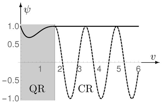 Figure 4. Joint representation of the HH-like QR-solution and the CR-solution , the latter being shown a second time in dashed style and with strong horizontal compression.Both in the HH-concept, used as a model, and in the present concept, the transition from the time-independent primordial state in four spatial dimensions to a time-dependent evolution in three spatial dimensions represents a critical point. (In the original version of the HH-concept [6], it appears somewhat non-transparent [17] by being accomplished via transition probabilities. In a later contribution—see pages 85–86 of Ref. [7]—the transition is explicitly performed by linking the purely spatial solution for the QR with the time-dependent solution for the CR, the same as done by us in this and in Section 3.2.1.)A look at the averaged probability density in the CR does not reveal why the DM should make this transition. In our case, it could slightly be favored by the fact that each of the four spatial coordinates and, in addition, coordinates resulting from them by a rotation (if allowed by LQG) are eligible for the transition to a time coordinate. However, another means can help: because a transition from space to time is concerned, it offers itself to relate the probability density in the CR to the time interval as in Section 3.2.1. According to Equation (23), due to the prefactor , starts with an extremely small value which is smaller than by many orders of magnitude. However, since it is a probability assessment of the same state, it must be considered as equivalent. In this way, the transition from space to time is associated with a corresponding change in relating the probability densities. Thus, the transition from purely spatial to time-dependent states finally leads to an evolution with increasing probabilities.
4. Critical Comments on the Quantum Results
4.1. Notes on the Storage and Transmission of Information
In Ref. [2], different possibilities have been indicated regarding how the information about the physical laws and their physical implementation could be stored in the DM. A storage in structured arrangements of space grains as examined in the LQG would seem most attractive. Unfortunately, due to the size of the smallest volume allowed by the LQG, i.e., the volume
of the space atoms according to page 30 or Ref. [18], this does not seem possible. In addition, the limits for the storage and transmission of information, determined by Bekenstein [19,20] and Bremermann [21], would also be infringed, provided that they were valid in the QR. Our “soft entry” process may serve as an example. The volume of the initial state after the entry is (see Figure 3) or
This corresponds fairly closely to the smallest volume (28) of the LQG, and, in that, according to the latter, substructures are not possible in which huge amounts of information could be stored. The mass of the DE contained in this volume is approximately where is the Planck mass. According to Bremermann, the upper limit for the information transmission speed is ≈. With an initial mass ≈ of the DM (reached after the “soft entry”) and a entry duration of ≈, the maximum transferable information is
which is far too little.
Despite the limitations of the LQG, let us at this point tentatively have a look at the possibility that, still undetected, much finer substructures below the LQG structures exist. (This is of course a rather speculative assumption.) After all, at least the WdW-Equation (A9),
allows such solutions. (In order to stay within the scope of valid physics, one would have to assume that the information concerned is not bound to matter. Otherwise, Bronstein’s black hole argument would be violated, according to which anything smaller than is “hidden inside its own mini black hole”, see pages 7–8 of Ref. [18]). A corresponding solution for the HH-like case with and, once again, is shown in Figure 5. (The discontinuous transition from short to extremely long waves is due to the fact that, in the transition from the QR to the CR, jumps from zero to , see Equation (10); it could be remedied by prescribing a continuous transition of .) Like the solution for the CR, it contains many zeros of , if . As for the CR-solution, we interpret the regions between neighboring zeros as single states. Except for those with small v, the distance between adjacent zeros is pretty much or , which can be derived from Equation (30): for , the latter reduces to
whence
and or
exactly. For , these are quanta of almost the same size as provided by the LQG according to Equation (28) with . (A spectrum of quanta can not be deduced here.) Equations (28) and (33) yield even the same volume quanta exactly, i.e., , if is chosen according to
Based on Equations (3) and (10), the same applies if for , while and are chosen according to
After Ref. [18], is a quantity of , from which it follows that . The latter is a conclusion that does not emerge from our investigation.
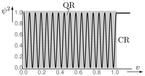
Figure 5.
QR-solution of Equation (30) with and substructures obtained by choosing . For the reason of presentability, only a small value, , was used. The short horizontal line at the top right is the beginning of .
Concerning our information problem, there are still other options to be considered. As already suggested in Ref. [2], information might also be stored in hidden higher dimensions, which would be an issue for string theory. Another possibility would be that both string and loop theory are involved. In the Discussion, Section 6, the urgency of the information problem is emphasized once again.
Another way of solving this problem, perhaps even the best one, would be to allow a much larger volume of the initial state. Even with an initial volume of the order (magnitude of the volume jumps of the classical solution), one would still be far in the range of quantum physics, albeit outside the range where QG is absolutely required. However, nothing seems to speak against using it there. This case of a much larger initial volume is addressed more closely in Section 4.3.
4.2. Notes on the Primordial States
According to Figure 3 and Figure 4, the width of the QR, resulting from solutions of Equation (14), is , essentially the same as found above for the volume quanta. This means that, in its primordial state, the DM consists of nothing more than a single space atom. If so, then the question arises as to whether it makes any sense to distinguish between solutions of different shape, e.g., a tunneling and a “soft entry” solution. This could at best serve to characterize space atoms of different shapes, but then should be done in a different way than usual. Furthermore, the question arises of whether the initial state for the classical evolution would not have to be composed of many space atoms. This possibility is discussed in the next subsection.
4.3. Primordial State with Large Volume
Figure 6 shows what the probability density of our “soft entry” process looks like when the QR is much further extended. As already indicated above, the size of the volume jumps performed by the classical solution appears to be a reasonable choice for the volume of the QR. The latter is then made up of about space atoms, which could be enough to accommodate the amount of information required by our DE model. For not having to choose a much smaller initial density (see Equation (3)) because of , we give up the condition for leading to the latter, and must replace the consequential boundary condition . This means that we can use Equation (14) and must only continue the “soft entry” solution underlying Figure 3 to larger values of v. For Figure 6, the position of the upper QR-boundary was chosen so that Equation (27) is satisfied. The transition from QR to CR would be best accomplished by passing over with continuous derivative to the decreasing density of the CR, and then looking for a common solution for the transition region, a lengthy procedure not accomplished here.
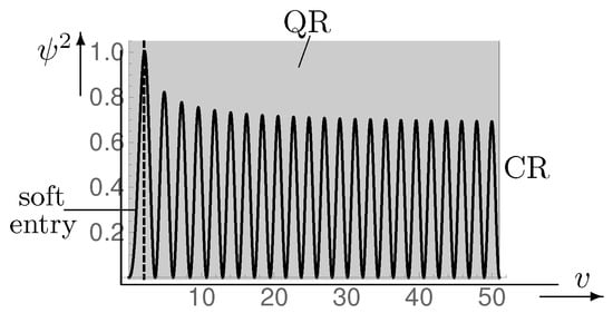
Figure 6.
Square of our “soft entry” solution, extending from to the dashed line, and at constant continued over a larger v-interval. The upper boundary value , selected for visualization, should in reality be much larger.
As can be seen from Figure 6, our “soft entry” solution fits very well with our interpretation of the -values between adjacent zeroes as quantum states. Obviously, the quantum states with small v-values are somewhat higher and wider than the others. This can be explained by the fact that they are subjected to a particularly strong spatial curvature. With the correspondingly continued HH-like state of Figure 4, the fit is not nearly as good. However, the extended “soft entry” state of Figure 6 can also be reinterpreted as HH-like. (For this purpose, Equation (27) was taken into account). For our purposes, this interpretation appears even more appropriate because it is difficult to imagine how large amounts of information will be accommodated, if the volume quanta, which are supposed to store them, arise one after the other.
The rather large volume of the HH-like primordial state thus obtained may even settle a never resolved discrepancy between the VL- and the HH-approach. According to Ref. [17], the VL-approach favors a universe (multiverse in our case) with an initial state of the smallest possible size, whereas the HH-approach favors one of the largest imaginable size. As a sort of compromise, our DM-model favors an HH-like primordial state of medium size between the smallest and largest possible.
5. Properties of the CR-Solution
5.1. Initial Equilibrium between DE and Matter
In Ref. [2], it was suggested that the initial state of the expansion phase could be an – albeit unstable – equilibrium between DE and matter. Because of the importance of this, the related calculation is made up here. For the sake of simplicity, it is limited to case . The additional matter term converts Equation (6) for into
With for , from this, we get
With , the time derivative of Equation (36) results in
In the case of the friction-involving interpretation, for and , this equation must reduce to Equation (5), i.e., . In consequence, in the last equation, must be replaced by . With the equilibrium conditions for , we get from the last equation
Resolving Equations (37) and (38) with respect to and yields the results shown in Table 1.

Table 1.
Equilibrium values of and .
Because in Ref. [1] the influence of an initial (unstable) equilibrium on the solutions has already been dealt with in detail, and because it is unlikely that, in the present case, significant changes will occur (due to the extremely slow temporal change of , the situation is already very equilibrium-like), and also for reasons of clarity, a correspondingly extended treatment is waved here.
5.2. Minimum Age of the Dark Multiverse
In Ref. [2], the age of the DM was evaluated on the simplifying assumption that its size exceeds that of U by a factor or more. This is far beyond the lower limit of , posed by measurements of the spatial curvature. Therefore, in the following, the age limit is determined. For this purpose, the factor in the solution (9) for must be taken from the full Equation (36) of Ref. [2], , where with presents a value of a and metric radius of the observable boundary of U. Putting and , we obtain from this equation
Inserting this, , with , and present Hubble time, in Equation (9) and resolving the latter with respect to yields its present value
In Figure 7, the function is shown together with the aforementioned lower limit .
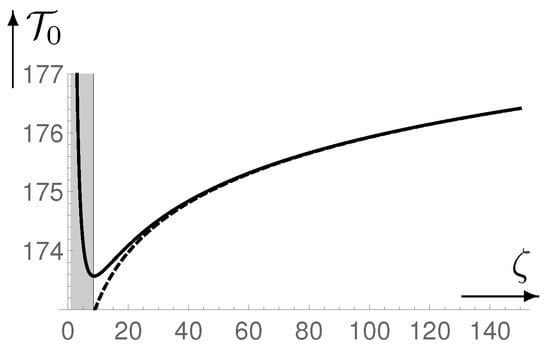
Figure 7.
Age of the DM as a function of . Due to inadmissible curvature values, the shaded area must be excluded. The dashed curve represents the approximation .
5.3. Irreversibility of the Friction-Involving Interpretation
By including the friction term in Equation (1), for particularized reasons (time savings for the transmission of information), an irreversible element was deliberately introduced into the basic cosmological equations derived from general relativity. It is surprising that the irreversible solutions thus obtained are also solutions of the usual equations involving a scalar field . It is worthwhile to investigate how this comes about. For this, we first consider the equations with a scalar field ,
All of them are invariant with respect to time reversal because appears in them only quadratically. ( is invariant because and change their sign simultaneously with t.)
Let us now turn to the irreversible interpretation involving friction. In this, the FL-Equation (2) is only seemingly reversible, since for . What was shown in Ref. [2] is that the solutions of this equation coincide with the solutions of the system of Equations (41) and (42) only as time is moving forward; for , this is no longer true. (This does not immediately become apparent from Ref. [2] because the solutions of the system (41) and (42) were only calculated forward in time. For example, Equation (60) from there, , used to calculate the solution, would have to be replaced by for .) The resolution of the seeming contradiction is therefore that the fulfillment of both the reversible and the irreversible equations by our solution applies only to advancing time.
5.4. Behavior of the DE in Our Universe
It was shown in Ref. [1] that the rest mass density of the DE, measured in M and U, matches for , where is the proper time in U, and is the time of the origin of U as judged from M. Our model assumes that in M the DE is at rest with respect to the coordinates , etc. This does not mean that it is at rest as well in U. It is shown below that it does so at least approximately.
In the following, we consider two states of U.
State 1: U contains only the DE of the DM, and, omitting the angular contributions, the square of the line element is
State 2: is the real present state of U with
where the subscript denotes the affiliation to U, is the radial, and the time-coordinate. We assume that the origins of the radial coordinates and coincide, and search for a transformation that converts into a form commensurable with . In order to keep an unchanged rest mass density, we set
With this (specifically ), from Equation (43), we get
where and are the partial derivatives of with respect to and resp. To determine how the position is judged in U, following from , we insert in this whence , and obtain
According to Equations (43) and (46), the differential contribution of an element to the distance of the position under consideration, expressed in terms of the radial coordinate of state 2, is . This is true because for length measurements, and according to Equation (45). With this, from Equations (44) and (46), we get or
where or is the distance from the origin of the DE-element at in situation 1 or 2 resp. According to this, the expansion velocity of the DE in U is
where was used. The expansion velocity of the cosmic substrate in U is
where was used, with H and being the Hubble parameter and the Hubble time resp. Inserting for the present value , with use of Equations (11), (48) and (49), and , the ratio of the two expansion velocities becomes
In view of uncertainties regarding the Hubble parameter and the huge numbers involved, it spoils nothing to say that the two velocities are essentially the same. Even a slightly larger expansion velocity of the DE cannot be excluded. In this case, the following scenario could come into effect: Since the observed expansion-acceleration of the material components of U is attributed to the DE, according to the principle actio = reactio, this should conversely delay the DE-expansion. The mass density of the DE could then even be slightly below the usual value because some of the acceleration caused by it would emanate from its kinetic energy. However, if the numerical values obtained above are correct, just the opposite will happen: a decelerating effect on the matter must be compensated by a slightly higher mass density of the DE.
6. Discussion
The concept of a timeless, spatially four-dimensional HH-like state developed in Section 3.1 and Section 3.2.2 as a primordial state represents one of the most important supplements to our model of the DM. In contrast to the tunneling or the “soft entry” concept, the information about the physical laws and the tools needed for their implementation are bound to matter from the very beginning. This can certainly be regarded as an advantage over the other two concepts, in which the tunneling or entry is preceded by a further state of pure information without integration into matter, a state that cannot be described within the framework of valid physical laws. According to Hawking, the HH-state could never have been created due to its timelessness because its creation would require a temporal before. The same argument would apply as well to our HH-like state. However, we cannot agree with this interpretation. It is certainly true that in many, perhaps most cases, cause and effect follow each other in time, which is usually associated with the use of these words. However, there are counterexamples in mathematics and logics, where, instead of cause and effect, the word pair precondition and consequence is used. In this case, the first implicates the second and not vice versa, with time being irrelevant. This is exactly what is also conceivable for the HH- or our HH-like state.
Because of its timelessness, like the HH-model, our HH-like model can only be treated within the framework of a QG-theory. Our unusual choice of a minisuperspace, using the volume as basis of the WdW-equation, was due to the fact that the usual procedure yields very implausible probabilities in the CR. Our approach leads not only to more plausible probabilities, but also to the identification of single states, which can be interpreted as spatial volume quanta.
With regard to the most important feature of our DM model, the storage and transmission of information about the physical laws, the investigations in Section 4.1 have shown how difficult it is to integrate deeper details beyond the friction term into common physics. On the other hand, it seems to be an urgent demand to open up new ways in this respect because the problem is palpable: elementary particles such as the electron have no receiving device and no brain, with which they could receive commands and implement them into action, and the properties with which they are described (e.g., rest mass, charge and spin) are not sufficient to act and react as required by physical laws. In this respect, at present, questions and speculations are instead the order of the day. As seen in Section 4.1, QG without loop theory would allow substructures below the LQG-structures. Would this be possible, or are the limits posed by LQG too restrictive? What role does the DE play in this game? At least the HH-like primordial state with large volume, treated in Section 4.3, seems to provide a useful approach.
Regarding newly identified properties of the solution for the CR, we point out the behavior of the DE in U, examined in Section 5.4. It is understood that DE causes the acceleration of galaxy expansion, and there must be a counteraction to this action. We suggested that the latter might consist in slowing down a somewhat higher expansion velocity of the DE, but this could not be conclusively demonstrated in consideration of very narrow numerical relationships and possible inaccuracies. Thus, after all, that too has to be ranked as a speculation. On the other hand, another, potentially disturbing problem with the friction term introduced into the equation for the DM-expansion-acceleration could be adequately solved.
As indicated at the beginning of the Introduction, it is currently a huge problem to prove beyond doubt that there is a multiverse at all and, even more so, to verify the validity of assumptions that enter into a multiverse concept. In our case, one possibility would be to examine more closely the footprint of the multiverse in our universe, specifically the time dependence of the DE density given by Equations (9) and (10). It would be even more difficult, but also more interesting, to unveil their decomposition into the two opposing components and given by Equation (2).
Funding
This research received no external funding.
Conflicts of Interest
The author declares no conflict of interest.
Abbreviations
The following abbreviations are used in this manuscript:
| M | multiverse |
| U | our universe |
| DE | dark energy |
| DM | dark multiverse |
| QR | quantum regime |
| CR | classical regime |
| VL | Vilenkin–Linde |
| HH | Hartle–Hawking |
| QG | quantum gravity |
| LQG | loop quantum gravity |
| WdW | Wheeler–de Witt |
| FL | Friedmann–Lemaître |
Appendix A
Inserting
in Equation (2) and multiplying the latter with yields
The case of constant density , examined closer in the main body, is included by setting and . Having the same dimension as , can be interpreted as an energy density. Integrating it at given a over the total volume V of the DM yields the quantity
Note that, by way of the multiplication by , the three-dimensionality of space enters decisively into the derivation. This is also expressed by the fact that and are 3D-densities. Interpreting H as the Hamiltonian of the system,
is the corresponding Lagrangian. The associated momenta are
(Since and result in Equations (41) and (42), our above interpretations of H and L are justified.) Resolving the last two equations with respect to and resp. and inserting the results into Equation (A3) with (A2) yields
Now, employing the quantisation rules and , after multiplication with we obtain the equation
where is the wave function of the DM in the so-called minisuperspace spanned by the variables a and . Inserting with , with dimensionless , , , and Equation (3) yields
In the case or , the substitutions and translate into and by what Equation (A7) reduces to the particularly simple and for frequently studied case
For the reasons depicted in Section 3.2, we do not employ this equation. Instead, we apply the equation which is obtained, if, in the above derivation, from Equation (A5) onward, a is eliminated by using , in place of , and a dimensionless volume . (The initial volume is , and the corresponding dimensionless volume is .) The result of this procedure is
It can be read directly from Equation (A8) by eliminating x through use of
and by replacing with . Note that Equation (A9) does not result from Equation (A8) simply through transformation and therefore has different solutions.
We are only dealing with real solutions in this paper, and for them the (also real) Hamiltonian is obviously Hermitian, no matter how the scalar product is defined. is the 3D-density of the probability P, i.e., so that its volume integral over the full range R of possible V values yields 1, i.e., we have
References
- Rebhan, E. Model of a multiverse providing the dark energy of our universe. Int. J. Mod. Phys. A 2017, 32, 1750149. [Google Scholar] [CrossRef]
- Rebhan, E. Acceleration of cosmic expansion through huge cosmological constant progressively reduced by submicroscopic information transfer. Int. J. Mod. Phys. A 2018, 33, 1850137. [Google Scholar] [CrossRef]
- Vilenkin, A. Creation of universes from nothing. Phys. Lett. B 1982, 117, 25–28. [Google Scholar] [CrossRef]
- Vilenkin, A. Quantum origin of the universe. Nucl. Phys. B 1985, 252, 141–152. [Google Scholar] [CrossRef]
- Linde, A.D. Quantum creation of the inflationary universe. Lett. Nuovo Cim. 1984, 39, 401–405. [Google Scholar] [CrossRef]
- Hartle, J.B.; Hawking, S.W. Wave function of the universe. Phys. Rev. B 1983, 28, 2960–2975. [Google Scholar] [CrossRef]
- Hawking, S.; Penrose, R. The Nature of Space and Time; Princeton University Press: Princeton, NJ, USA, 2000. [Google Scholar]
- DeWitt, C.M.; Wheeler, J.A. (Eds.) Lectures in Mathematics and Physics. In Batelle Rencontres; Benjamin: New York, NY, USA, 1968. [Google Scholar]
- DeWitt, B.S. Quantum Theory of Gravity. I. The Canonical Theory. Phys. Rev. 1967, 160, 1113–1148. [Google Scholar] [CrossRef]
- Coleman, S. Why there is nothing rather than something: A theory of the cosmological constant. Nucl. Phys. B 1988, 310, 643–668. [Google Scholar] [CrossRef]
- Linde, A. Particle Physics and Inflationary Cosmology; Contemporary Concepts Physics 5; Harwood Academic Publishers: Reading, UK, 1990; pp. 1–362. [Google Scholar]
- Rovelli, C. Reality Is Not What It Seems: The Journey to Quantum Gravity; Penguin Publishing Group: London, UK, 2017. [Google Scholar]
- Vilenkin, A.; Yamada, M. Tunneling wave function of the universe. arXiv 2018, arXiv:1808.02032v2. [Google Scholar] [CrossRef]
- Peres, A. Critique of the Wheeler-DeWitt Equation. In On Einstein’s Path. Essays in Honor of Engelbert Schucking; Harvey, A., Ed.; Springer: New York, NY, USA, 1999; pp. 367–379. [Google Scholar]
- Patrick, P. Using Trajectories in Quantum Cosmology. arXiv 2018, arXiv:1902.00796v1. [Google Scholar]
- Pinto-Neto, N.; Fabris, J.C. Quantum cosmology from the de Broglie–Bohm perspective. Class. Quantum Gravity 2013, 30, 143001. [Google Scholar] [CrossRef]
- Vilenkin, A. Many Worlds in One; Hill and Wang: New York, NY, USA, 2006; pp. 190–191. [Google Scholar]
- Rovelli, C.; Vidotto, F. Covariant Loop Quantum Gravity: An Elementary Introduction to Quantum Gravity and Spinfoam Theory; Cambridge University Press: Camebridge, UK, 2014; Available online: http://www.cpt.univ-mrs.fr/~rovelli/IntroductionLQG.pdf (accessed on 27 May 2019).
- Bekenstein, J.D. Universal upper bound on the entropy-to-energy ratio for bounded systems. Phys. Rev. D 1981, 23, 287. [Google Scholar] [CrossRef]
- Bekenstein, J.D. Energy cost of information transfer. Phys. Rev. Lett. 1981, 46, 623–626. [Google Scholar] [CrossRef]
- Bremermann, H.J. Optimization through evolution and recombination. In Self-Organizing Systems 1962; Yovits, M.C., Jacobi, G.T., Goldstein, G.D., Eds.; Spartan Books: Washington, DC, USA, 1962; pp. 93–106. [Google Scholar]
| 1 | For later purposes (Section 4.1), we consider here a slightly more general case. Unfortunately, when Ref. [2] was written down for printing, in the derivation of Equation (26) there (Equation (7) here), two different types of calculation were mixed up, which resulted in two sign errors. For correction, the following substitutions must be made there: in Equation (22), and in the unnumbered equation immediately thereafter. The resulting Equation (26) is, however, correct. |
| 2 | Note that by this assumption or resp. the term in Equation (2) drops out, i.e., the friction term plays a role only in the CR. |
| 3 | Due to space-related quantum effects, this number could be quite small. |


© 2019 by the author. Licensee MDPI, Basel, Switzerland. This article is an open access article distributed under the terms and conditions of the Creative Commons Attribution (CC BY) license (http://creativecommons.org/licenses/by/4.0/).