Averaging and the Shape of the Correlation Function

Abstract

A brief pedagogical introduction to correlation femtoscopy is given. We then focus on the shape of the correlation function and discuss the possible reasons for its departure from the Gaussian form and better reproduction with a Lévy stable distribution. With the help of Monte Carlo simulations based on asymmetric extension of the Blast-Wave model with resonances we demonstrate possible influence of averaging over many events and integrating over wide momentum bins on the shape of the correlation function. We also show that the shape is strongly influenced by the use of the one-dimensional parametrisation in the $q_{inv}$ variable.

1. Introduction

Correlation femtoscopy is widely used in heavy-ion collisions for the determination of space–time characteristics of hadron-emitting sources. Most commonly, the two-particle correlation functions are fitted by a Gaussian parametrisation augmented with correction terms due to final-state interactions. The widths of this parametrisation are interpreted in terms of space–time (co-)variances of the homogeneity regions [1,2,3,4,5].

Nevertheless, clear indications exist, that the real shape of the correlation function is not Gaussian, as we could also see in a few talks at the 2018 Zimányi School (see e.g., [6,7,8]). The shape is often better reproduced by a fit with Lévy stable distribution [9]. The choice of this distribution is not random. Stability is a generalisation of the concept of Central Limit Theorems. Lévy stable distributions possess the property that the shape remains unchanged when one more elementary random process is added to the ones which are already accounted for. The excitement about this particular parametrisation is supported by the argument that with the help of such a fit one could access the critical exponents of the strongly interacting matter [10]. We will show in this paper that the observed shape can be caused by more mundane non-critical phenomena. Mostly, we are interested in the role of averaging in influencing the shape of the correlation function. Note that here we shall only be interested in correlation functions from nuclear collisions.

These ideas set out the outline of this contribution. We first review the basic relations of correlation femtoscopy. Then we particularly look at the Lévy stable parametrisations and scrutinise various effects that can lead to such a shape of the correlation function.

2. The Formalism of Correlation Femtoscopy

The two-particle correlation function is constructed in such a way as to reveal the effect of correlations. Since this is a school, we stay on a pedagogical level and introduce the main elements of correlation femtoscopy one by one. For pion pairs one usually uses the correlation stemming from the symmetrisation of the wave function. Nevertheless, the effect of final state interactions is always present, as well. They can be due to electromagnetic or strong interactions. For identical charged pions, the electromagnetic Coulomb final state interactions are important. We shall assume here, that their influence can be factored out from the data with the help of a correction factor [11,12].

The correlation function is then experimentally obtained as

$$C(p_1,p_2)=\frac{P(p_1,p_2)}{P_{\mathrm{mix}}(p_1,p_2)},$$

(1)

where $P(p_1,p_2)$ is the two-particle distribution in the momenta, and $P_{\mathrm{mix}}(p_1,p_2)$ is an analogous distribution in which each particle comes from a different event. Due to wave function symmetrisation for boson pairs, the correlation function exhibits a peak for small momentum differences $p_1-p_2$, provided that Coulomb repulsion can be filtered out. Thus it is more convenient to study the dependence of the correlation function on the momentum difference and the average momentum

$$q=p_1-p_2,K=\frac{1}{2}\left(p_1+p_2\right).$$

(2)

The source, which produces particles, can be described with the help of a Wigner density $S(x,p)$. Its classical interpretation is that it is the probability to emit a particle with momentum p from a space–time point x. The correlation function which we express as function of q and K is then given as

$$C(q,K)-1\approx \frac{{\left|\int d^{4}xS(x,K)e^{iqx}\right|}^2}{{\left(\int d^{4}xS(x,K)\right)}^2}.$$

(3)

The approximation symbol stands here for two steps: (i) The on-shell approximation which replaces the time-component of $K^0$ ($=(p_1^0+p_2^0)/2$) with $E_K=\sqrt{{\overrightarrow{K}}^2+m^2}$, and (ii) the smoothness approximation, which assumes that the denominator can be evaluated at single value of K instead of the two momenta of the particles of the pair: $p_1=K+q/2$ and $p_2=K-q/2$. After some manipulations the relation can be rewritten as a simple Fourier transform:

$$C(q,K)\approx 1+\frac{\int d^{4}rD(r,K)e^{iqr}}{{\left(\int d^{4}xS(x,K)\right)}^2},$$

(4)

where

$$D(r,K)=\int d^{4}XS\left(X+\frac{r}{2},K\right)S\left(X-\frac{r}{2},K\right).$$

(5)

We see that the correlation function does not measure the distribution of the source itself. Instead, it is a Fourier transform of the distribution of the differences between emission points! This is important! The convolution in Equation (5) often produces a bell-shaped distribution $D(r,K)$ even for emission functions which might possess sharp edges. The Fourier transform in Equation (4) keeps this feature. This is the reason why fitting the correlation function with Gaussian does not seem such a bad idea.

Unfortunately, even measurement of the distribution $D(r,K)$ is not completely possible. Since the momenta of the particles used in the measurement must fulfil the mass-shell constraint, we have

$$q·K=0\Rightarrow q^0=\frac{\overrightarrow{q}·\overrightarrow{K}}{K^0}=\overrightarrow{q}·\overrightarrow{\beta }$$

(6)

where

$$\overrightarrow{\beta }=\frac{\overrightarrow{K}}{K^0}\approx \frac{\overrightarrow{K}}{E_K}.$$

(7)

Hence, only three components of q are independent.

In order to exploit the symmetries of the problem and simplify the interpretation of the measurement, one adopts the out-side-long coordinate frame. The longitudinal (or z) direction is parallel to the beam. The outward (or x) direction is identified with the direction of the transverse pair momentum $K_T$, so that $\overrightarrow{K}=(K_T,0,K_l)$. The sideward (or y) direction is perpendicular to the above two. In this frame the Gaussian parametrisation of the correlation function reads

$$C(q,K)-1=exp\left[-q_o^2{R}_o^2-q_s^2{R}_s^2-q_l^2{R}_l^2-2q_o{q}_s{R}_{os}^2-2q_o{q}_l{R}_{ol}^2-2q_s{q}_l{R}_{sl}^2\right].$$

(8)

If this parametrisation is expanded up to second order in q and compared with such an expansion of Equation (3), one recovers the model-independent expressions for the correlation radii [13]

$$\begin{array}{cccc}\hfill R_o^2& =〈{(\tilde{x}-{\beta }_T\tilde{t})}^2〉,\hfill & \hfill R_{os}^2& =〈(\tilde{x}-{\beta }_T\tilde{t})\tilde{y}〉,\hfill \\ \hfill R_s^2& =〈{\tilde{y}}^2〉,\hfill & \hfill R_{ol}^2& =〈(\tilde{x}-{\beta }_T\tilde{t})(\tilde{x}-{\beta }_l\tilde{t})〉,\hfill \\ \hfill R_l^2& =〈{(\tilde{z}-{\beta }_l\tilde{t})}^2〉,\hfill & \hfill R_{sl}^2& =〈\tilde{y}(\tilde{z}-{\beta }_l\tilde{t})〉.\hfill \end{array}$$

(9)

Here, the averages are taken with the emission function

$$\langle f(x)\rangle (K)=\frac{\int d^{4}xf(x)S(x,K)}{\int d^{4}xS(x,K)},$$

(10)

and the coordinates with the tilde are shifted with respect to the means

$$\tilde{x}=x-\langle x\rangle .$$

A caveat must be placed here in connection with the Expressions (9). They are well defined as long as the (co)variances of the emission function can be calculated. If the emission function, however, would be given by a Lévy stable distribution, they would not exist and the interpretation would fail. Moreover—the interpretation is even more complicated: Below we discuss how the measured correlation function results from averaging over different (effective) sources, so strictly speaking no single emission function can be assigned to the measured correlations. Nevertheless, let us consider the Expressions (9) as useful guidelines for the interpretation of measured Gaussian correlation radii.

Sometimes, poor statistics does not allow to sample the q-space densely enough with data so that a decent fit to the histogram can be made. In this case, a one-dimensional parametrisation of the correlation function is sometimes used, which is formulated in terms of the invariant momentum difference

$$q_{inv}^2=q_o^2+q_s^2+q_l^2-q_0^2={\left|\overrightarrow{q}\right|}^2-{(\overrightarrow{q}·\overrightarrow{\beta })}^2.$$

(11)

In order to calculate the correlation function $C(q_{inv},K)$ one would need to integrate both the numerator and the denominator of the three-dimensional $C(q,K)$ separately over the hypersurface in q-space

$$C(q_{inv},K)=1+\frac{\int d{q}_{o}d{q}_{s}d{q}_l\delta (|\overrightarrow{q}{|}^2-{(\overrightarrow{q}·\overrightarrow{\beta })}^2-q_{inv}^2){\left|\int d^{4}xS(x,K)e^{iqx}\right|}^2}{\int d{q}_{o}d{q}_{s}d{q}_l\delta (|\overrightarrow{q}{|}^2-{(\overrightarrow{q}·\overrightarrow{\beta })}^2-q_{inv}^2){\left(\int d^{4}xS(x,K)\right)}^2}.$$

(12)

Note that we still assume the validity of the smoothness and the on-shell approximations.

This can be most easily interpreted in the reference frame which co-moves with the particle pair, i.e., with the velocity $\overrightarrow{\beta }$. There, all terms which contain $\overrightarrow{\beta }$ vanish, and the correlation function becomes

$$C(q_{inv},K)=1+\frac{\int d{q}_{o}d{q}_{s}d{q}_l\delta (|\overrightarrow{q}{|}^2-q_{inv}^2){\left|\int d^{4}xS(x,K)e^{iqx}\right|}^2}{\int d{q}_{o}d{q}_{s}d{q}_l\delta (|\overrightarrow{q}{|}^2-q_{inv}^2){\left(\int d^{4}xS(x,K)\right)}^2}.$$

(13)

If the modification is done on the level of Gaussian parametrisation

$$C(q_{inv},K)=1+\frac{1}{\mathcal{N}}\int d{q}_{o}d{q}_{s}d{q}_l\delta (|\overrightarrow{q}{|}^2-q_{inv}^2)exp\left(-q_i{q}_j\langle x^i{x}^j\rangle \right),$$

(14)

where

$$\mathcal{N}\equiv \int d{q}_{o}d{q}_{s}d{q}_l\delta (|\overrightarrow{q}{|}^2-q_{inv}^2)$$

(15)

ensures that the normalization of the correlation function is unaffected by integral over the q-surface. Hence, in this frame the averaging runs over the q-surface with constant $|\overrightarrow{q}|$. The observed width of $C(q_{inv},K)$ results from this averaging.

The value of $q_{inv}$ can become 0 (where one would expect the maximum of the correlation function) also for non-vanishing q components (where the maximum is not expected). Therefore, a new variable has been introduced [14]

$$q_{LCMS}={\left(q_o^2+q_s^2+q_{l,LCMS}^2\right)}^{1/2}\mathrm{where}{q}_{l,LCMS}^2=\frac{{(p_{1z}{E}_2-p_{2z}{E}_1)}^2}{K_0^2-K_l^2}.$$

(16)

Note that $q_{LCMS}$ is invariant under longitudinal boosts. The motivation for this particular variable is that in the longitudinally co-moving frame ($K_l=0$) it reduces just to $\sqrt{q_o^2+q_s^2+q_l^2}$. This variable is thus reasonable for spherically symmetric sources. We have checked that there is no dramatic qualitative difference between the results obtained with $q_{inv}$ and those obtained with $q_{LCMS}$ [15]. Here we shall show results obtained with $q_{inv}$, while results with $q_{LCMS}$ will be shown elsewhere [15].

We have indicated in Equation (10) that the measured (co-)variances of the source depend on the pair momentum K. Why? The reason is that the particles with specified momentum only come from a part of the whole fireball, the so-called homogeneity region. If we change the momentum K, i.e., we focus on particles with different momentum, then these will be emitted from a different part of the fireball. That part also may have different size. Consequently, the sizes of the (co-)variances in Equation (9) change.

3. Averaging

We shall deal with two kinds of averaging in the discussions of the shape of the correlation function: Averaging over different momenta and averaging over many events.

Averaging over momentum comes through the binning in pair momentum K. Both histograms in q—the numerator and the denominator in Equation (1)—are constructed for $\overrightarrow{K}$ within certain interval. The bins always have finite size in the transverse component as well as in the azimuthal angle of $\overrightarrow{K}$. The latter is often even integrated over the whole $2\pi$ interval. As we pointed out, the correlation function measures the homogeneity lengths corresponding to a given $\overrightarrow{K}$. Then by taking an interval of $\overrightarrow{K}$ one makes an average over different homogeneity regions. Since the intervals of $\overrightarrow{K}$ are integrated on the level of the two histograms in Equation (1), the resulting correlation function is given as

$$C(q,K)\approx 1+\frac{{\int }_{bin}dK{\left|\int d^{4}xS(x,K)e^{iqx}\right|}^2}{{\left({\int }_{bin}dK\int d^{4}xS(x,K)\right)}^2}.$$

(17)

Averaging over events results from summing up entries to the histograms from a large number of events. Both the numerator and the denominator fluctuate from event to event, because in each event we have a fireball of different sizes and dynamical state. Averaging must therefore be carried out for the numerator and denominator separately [16,17]. We thus conclude that the correlation function will be

$$C(q,K)\approx 1+\frac{\int dR\rho (R){\left|\int d^{4}xS(x,K;R)e^{iqx}\right|}^2}{\int dR\rho (R){\left(\int d^{4}xS(x,K;R)\right)}^2}$$

(18)

where $\rho (R)$ is the distribution of the source sizes. For brevity, we do not write out the averaging over other features of the fluctuating source explicitly; this would be implemented in the same way.

A non-Gaussian shape of the correlation function will be here fitted with the Lévy stable distribution. In one dimension is reads

$$C(q)=1+\lambda e^{-{(qR)}^{\alpha }}.$$

(19)

The three-dimensional generalisation can be formulated as [9]

$$C(q)=1+\lambda e^{-{(q_o^2{R}_o^{\prime 2}+q_s^2{R}_s^{\prime 2}+q_l^2{R}_l^{\prime 2})}^{\alpha /2}}.$$

(20)

The Lévy exponent $\alpha$ is one of the fit parameters, together with $\lambda$ and the $R^{\prime }$’s. The value $\alpha =2$ corresponds to Gaussian shape, meaning that a lower value ($\alpha <2$) implies a non-Gaussian correlation function.

4. The Blast-Wave Model

For the actual calculation of various effects we will generate artificial events with the help of DRAGON Monte Carlo event generator [18,19]. It is based on the Blast-Wave (BW) model [20,21,22,23,24] with resonance decays included. The BW model is described by the emission function

$$S(x,K)d^{4}x=\frac{1}{{(2\pi )}^3}{\left(exp\left(\frac{u^{\mu }(x)p_{\mu }}{T}\right)\pm 1\right)}^{-1}\mathsf{\Theta }(r-R(\theta ))\delta (\tau -{\tau }_{fo})m_{t}cosh(\eta -y)\tau d\tau d\eta rdrd\theta .$$

(21)

As spatial coordinates we use here the usual polar coordinates r and $\theta$ for the plane transverse to the beam direction, the space–time rapidity $\eta$ and the longitudinal proper time $\tau$

$$\eta =\frac{1}{2}ln\frac{t+z}{t-z},\tau =\sqrt{t^2-z^2}.$$

(22)

Let us explain the formula representing this particular emission function.

• The factor ${(2\pi )}^{-3}$ stands for the elementary phase-space cell volume. Recall that $S(x,K)$ represents the distribution in phase-space. (And recall that $\hslash =c=1$.)
• The thermal distribution—Bose-Einstein or Fermi-Dirac—is formulated with the energy in the rest frame of the fluid, $E^{*}=u^{\mu }{p}_{\mu }$, where $u^{\mu }$ is the (local) velocity of the fluid.
• The fireball is modelled with a sharp cutoff in the transverse direction: $\mathsf{\Theta }(r-R(\theta ))$. However, the radius R depends on the azimuthal angle in order to simulate the fireball in non-central collisions.
• Freeze out happens along a hypersurface given by constant $\tau ={\tau }_{fo}$.
• The fireball is manifestly boost-invariant. There is no limit set on the space–time rapidity. Nevertheless, by choosing the rapidity of particles one effectively selects just a part of the fireball (the relevant homogeneity region) which contributes to the production at that rapidity.
• The factor $m_{t}cosh(\eta -y)\tau d\tau d\eta rdrd\theta$, where y is the rapidity of the emitted particle, comes from the Cooper-Frye [25] factor which stands for the flux of particles across the freeze-out hypersurface $\mathsf{\Sigma }$: $p_{\mu }d{\mathsf{\Sigma }}^{\mu }$.

Our model does not include any corrections to the thermal momentum distribution due to viscosity.

The transverse radius of the fireball depends on the azimuthal angle in order to implement the second-order anisotropy

$$R(\theta )=R_0\left[1-a_{2}cos\left(2(\theta -{\theta }_2)\right)\right],$$

(23)

where $R_0$ and $a_2$ are model parameters, and ${\theta }_2$ is the angle of the second-order event plane.

The collective expansion velocity field is parametrised with the help of $\eta$ and the transverse rapidity ${\eta }_t(r,{\theta }_b)$

$$u^{\mu }(x)=(cosh\eta cosh{\eta }_t(r,{\theta }_b),cos{\theta }_{b}sinh{\eta }_t(r,{\theta }_b),sin{\theta }_{b}sinh{\eta }_t(r,{\theta }_b),sinh\eta cosh{\eta }_t(r,{\theta }_b)),$$

(24)

where the transverse rapidity depends on r and the azimuthal angle

$${\eta }_t(r,{\theta }_b)={\rho }_0\frac{r}{R(\theta )}\left[1+2{\rho }_{2}cos(2({\theta }_b-{\theta }_2))\right].$$

(25)

The model parameters ${\rho }_0$ and ${\rho }_2$ scale the overall magnitude and the second-order oscillation of the transverse flow, respectively. We have indicated that ${\eta }_t$ depends on ${\theta }_b$, and not directly on $\theta$. The angle ${\theta }_b$ gives the direction perpendicular to the surface of the fireball, and can be obtained from the relation

$$tan\left({\theta }_b-\frac{\pi }{2}\right)=\frac{d{x}_2}{d{x}_1}=\frac{\frac{d{x}_2}{d\theta }}{\frac{d{x}_1}{d\theta }}=\frac{\frac{dR(\theta )sin(\theta )}{d\theta }}{\frac{dR(\theta )cos(\theta )}{d\theta }},$$

(26)

where the functional dependences $x_1(\theta )$, $x_2(\theta )$ refer to the transverse boundary of the fireball [26].

DRAGON also includes resonance decays. Mesonic resonances are included up to masses of 1.5 GeV, baryonic up to 2 GeV. Resonances are produced according to the same emission function as direct pions, with their pole masses. The decay vertex of a given resonance is determined according to an exponential distribution whose width is the lifetime of the resonance in question (in its rest frame): $\rho ({\tau }_d)\propto e^{-{\mathsf{\Gamma }}_R{\tau }_d}$. Both two- and three-body decays are included as well as the possibility that one resonance type can decay via various channels according to their branching ratios. Cascades of decays, in which several resonances decay consecutively, are also possible within the model.

5. Results

We begin by considering the effects that the averaging over many fireballs with different shapes may have on the value of the Lévy parameter $\alpha$. Indeed, in real experiments each fireball is different, with different sizes, eccentricities, and orientations of the event plane. We therefore anticipate that averaging over a distribution of source shapes, as in Equation (18), will cause $\alpha$ to deviate from 2. In this treatment, we limit our focus to second-order anisotropies.

With the help of DRAGON we generated sets of 50,000 events. The basic setting of the parameters includes the freeze-out temperature of 120 MeV, the average transverse radius $R=7$ fm, freeze-out time ${\tau }_{fo}=10$ fm/c, and the strength of the transverse expansion ${\rho }_0=0.8$. To keep the source simple, no resonance decays are included at this point. The correlation function is evaluated in one dimension as a function of $q_{inv}$.

We first study the effect of averaging over different values of $a_2$.

Figure 1 (left) compares the Lévy parameter $\alpha$ from two sets of Monte Carlo events. In the first set, all events have spatial eccentricity with $a_2=0.05$. In the other set, the eccentricity fluctuates with $a_2$ between $-0.1$ and $0.1$. We perform the study in a narrow interval of $K_T$, where the shape of the correlation function changes strongly, even though it cannot be accessed experimentally (although the correlation function has been averaged over the azimuthal angle of $\overrightarrow{K}$). We see that the value of $\alpha$ departs from 2 considerably and reaches values between 1.27 and 1.62. The averaging makes up only a small portion of this decrease, at most at a level of 0.05.

Almost identical results quantitatively come from the averaging over flow anisotropy (Figure 1, middle) and the event plane orientation (Figure 1, right). In the middle panel we compare Lévy index $\alpha$ obtained from a set with ${\rho }_2$ fixed to 0.05 with a set with events for which ${\rho }_2$ fluctuates between $-0.1$ and $0.1$. For the event plane averaging we see no change (except in the bin with smallest $K_T$) if ${\theta }_2$ fluctuates in comparison to ${\theta }_2$ fixed to 0. The anisotropy parameters $a_2$ and ${\rho }_2$ in this case fluctuate between $-0.1$ and $0.1$.

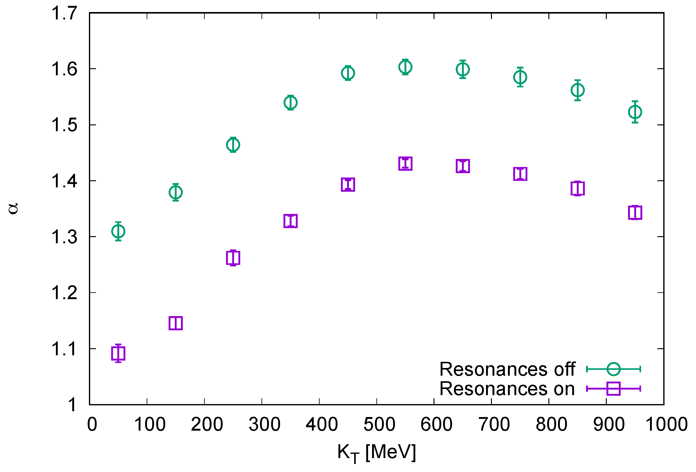
We investigate next the influence of resonances on the obtained value of $\alpha$. We use the source of direct particles with the same basic parameters as in the previous case, and we compare correlation functions obtained with and without resonance decays.

In Figure 2 we show the Lévy indices $\alpha$ obtained from fits to the correlation functions as a function of $K_T$. We know from the previous Figure already, that the one-dimensional correlation function has quite a non-Gaussian shape. Now we see that the inclusion of the resonance decays pushes down the value of $\alpha$ by another 0.2. The influence of resonance decays is much bigger than that of averaging over different events!

We want to perform our analysis more differentially, however. We start by looking individually at each direction of the correlation function and fitting with the Lévy prescription of Equation (19). This is not a three-dimensional analysis, since we do not fit the correlation function in the whole q-space and confine ourselves only to fits along the axes. The aim is to see the differences in its shape along different directions.

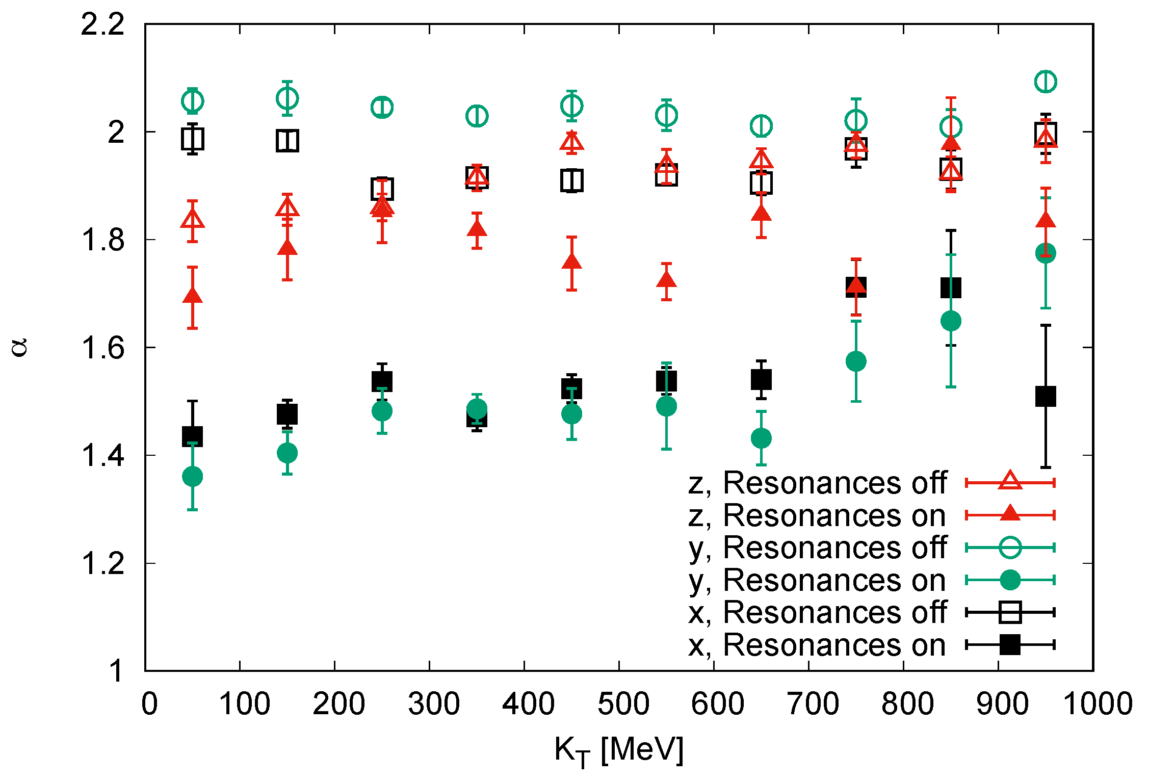
Indeed, we observe in Figure 3 that the differences are rather large. If resonance decays are not included, the value of $\alpha$ is around 2 in both transverse directions. However, in the longitudinal direction the Lévy index $\alpha$ is lowered to 1.8 at $K_T=0$ and increases gradually towards 2 at $K_T=1$ GeV. In addition, the influence of resonance decays is different for longitudinal and transverse directions. In the longitudinal direction the resonance decays cause a decrease of $\alpha$ by about 0.2. In the transverse directions, however, $\alpha$ drops as low as 1.4 once resonance decays are included.

Note the wiggly behaviour of the data points, particularly for larger $K_T$. Due to the limited statistics of particle pairs, the measured values of the correlation function will tend to fluctuate. The parameter $\alpha$ comes from the fit to the correlation function with Equation (19). The error bars show the $\pm 1\sigma$ intervals for this particular correlation function. They underestimate the real uncertainty of the determination of $\alpha$. We plan to improve the statistics and the uncertainty intervals in a forthcoming paper [15].

We would like to understand these differences and hence we checked the shape of the source which emits pions.

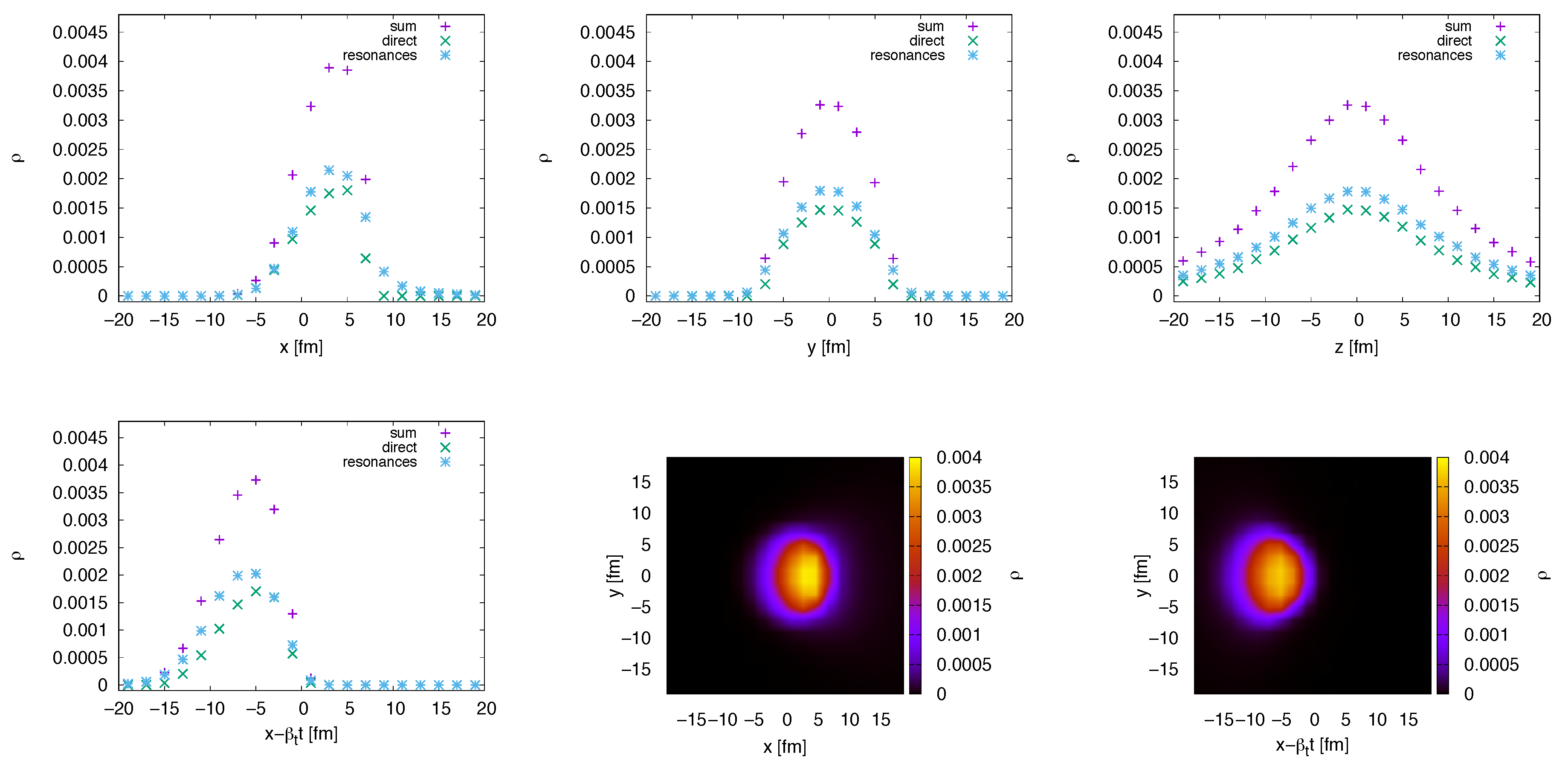
The profiles of the emission function are plotted in Figure 4, for pions with transverse momentum from the interval (300, 400) MeV. Note that they are produced just from a part of the whole fireball, the so-called homogeneity region. We show the distribution of the production points of pions, with pions from resonance decays included. In order to assess the effect of resonances, we also plot separately both contributions: Directly produced pions as well as those from resonance decays. The upper row shows that there is quite a difference between the longitudinal and the transverse directions. One could argue, however, that due to the on-shell constraint (6) it is not the distribution in x, that is measured, but rather the distribution in $(\mathrm{x}-{\beta }_{t}t)$. We plot this in the lower left panel of Figure 4.

At this place we would again like to touch upon the discussion concerning the proper choice of the one-dimensional momentum difference variable ($q_{inv}$ vs. $q_{LCMS}$). We recall that $q_{LCMS}$ was introduced as a reasonable variable for spherically symmetric sources. Figure 4 shows that in this case the symmetry is not present, neither concerning the sizes, nor concerning the shape of the source in different directions.

Finally, we extend the fitting to the whole three-dimensional correlation function from the previous simulations. The fit is performed with the three-dimensional Lévy distribution of Equation (20), so it always results in a single value of $\alpha$.

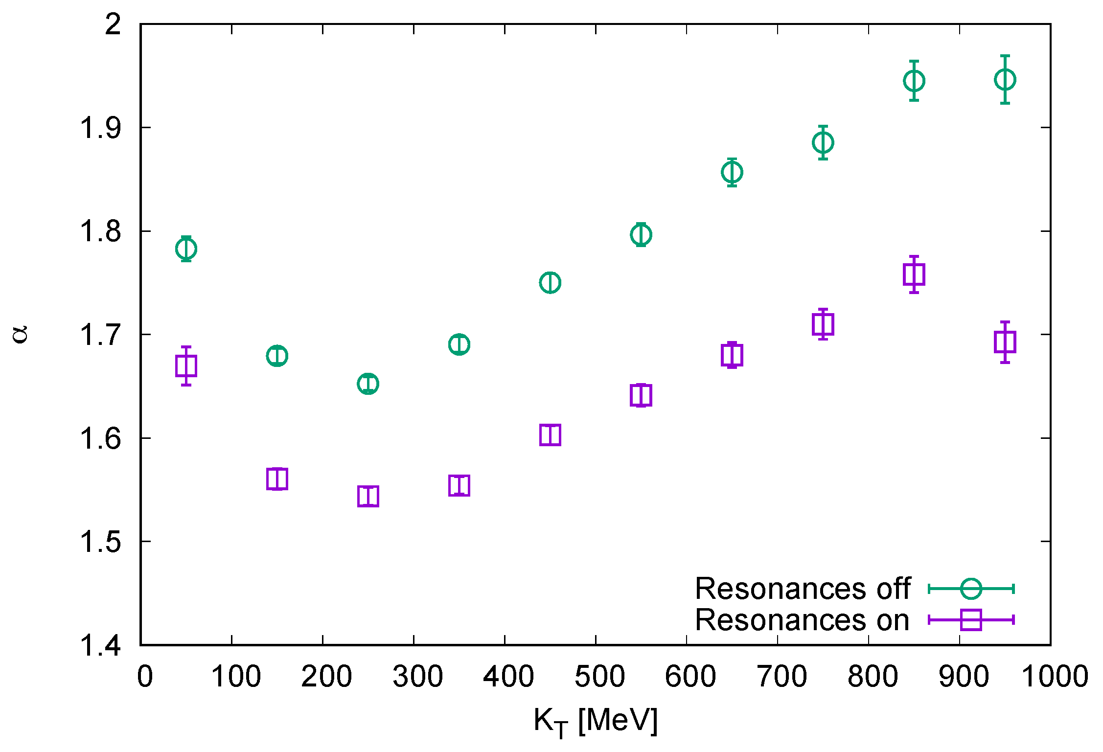
This is plotted in Figure 5 as a function of $K_T$. We can see that the obtained $\alpha$’s are closer to 2 than in the case of fitting the one-dimensional correlation functions in $q_{inv}$, although considerable deviations from 2 are still present. Inclusion of resonance decays lowers $\alpha$ by about 0.1–0.3, depending on $K_T$.

6. Conclusions

We explained in the introductory section of this paper that in addition to the generalisation of the concept of Central Limit Theorem [9], an especially important motivation for the use of Lévy stable parametrisation is the search for critical behaviour [10]. The simulations presented here show that the Lévy parameter $\alpha$ may clearly deviate from 2 even for “usual”, non-critical sources, like those described by the blast-wave model.

Even without the presence of resonances, the shape of the correlation function looks rather non-Gaussian in the longitudinal direction. Once resonance decays are included, however, the shape deviates even further from Gaussian, especially in the two transverse directions. In this respect it appears interesting to test this with kaons, since a smaller part of them (although not negligible) comes from resonance decays.

In the three-dimensional fit, the value of $\alpha$ is lowered through the influence of resonance decays by about 0.1–0.3, depending on $K_T$.

It is very important to realise that in our simulations the biggest effect on lowering the value of $\alpha$ was in using only one-dimensional parametrisation of the correlation function in $q_{inv}$.