1. Quark Condensate for Various Heavy Flavors
As is well known, because of confinement in QCD, quarks and gluons do not exist as individual particles, but appear only in the form of bound states (for recent reviews, see [
1,
2]). The latter include mesons, baryons (as well as other possible quark bound states, such as tetra- and pentaquarks), glueballs, and the so-called hybrids consisting of a quark, an antiquark, and one or several gluons. Each bound state can be represented as an average of a certain operator over the Euclidean QCD vacuum. Since the vacuum state is gauge-invariant, only the gauge-invariant operators yield non-vanishing results once averaged over it. (This statement can be viewed as a corollary of the so-called Elitzur theorem [
3,
4], which states that a local gauge symmetry cannot be broken spontaneously.) For local composite operators, such as
or
, gauge invariance holds automatically, and the mean values of these operators yield the QCD condensates [
5,
6]. Nevertheless, the quark and the gluon bound states are in general represented by the field operators which are defined at different points of the Euclidean space, so that a phase factor (also called a parallel transporter or a Schwinger string) interpolating between these points is required in order to provide gauge invariance of the full non-local operator. That is, the non-local gauge-invariant operators have, e.g., the form
where
and
are the phase factors transforming under the fundamental and the adjoint representations of SU(
N), respectively, with
and
. (Throughout this review, we denote the number of colors by
N.) Thus, the phase factors provide long-range correlations of color between individual quark operators
ψ and
, as well as the gluonic field strengths
, thereby making the non-local operators (
1) gauge invariant. (Note, however, that, in spite of their gauge invariance, the operators (
1) still depend on the shape of a contour that enters the phase factor
or
.) Such long-range correlations of color are associated with confining interactions between the constituents of the QCD bound states. By accounting for confinement of gauge particles which propagate in the loops, one can arrive at the results inaccessible within the conventional perturbation theory, such as the infra-red finiteness of the running strong coupling. The world-line representation for the Green function of a particle, which propagates along a closed Euclidean trajectory and interacts with quantum gauge fields, contains a Wilson-loop average. In general, the corresponding world-line integral cannot be calculated analytically, because finding the minimal surface for an arbitrary contour
in
dimensions is too complicated. For this reason, effective parametrizations of the minimal surface have been invented in the literature [
7,
8,
9] in order to construct the minimal-area functional in terms of
. Owing to the fact that the Wilson-loop average is fully defined in terms of the geometric characteristics of the contour
, this approach has an advantageous feature of being able to reduce the calculation of vacuum amplitudes in QCD to the calculation of the world-line integrals in an effective Abelian gauge theory, or even in quantum mechanics.
We start demonstrating these ideas at an example of the calculation of the heavy-quark condensate [
10]. Numerically, the wavelengths of the heavy, i.e.,
c-,
b-, and
t-, quarks are smaller than the Yang-Mills vacuum correlation length
λ (see the details below), so that the typical Euclidean trajectories of these quarks fit into a circle of diameter
λ. To calculate the corresponding small-sized Wilson-loop average, one can use the non-Abelian Stokes’ theorem and the cumulant expansion to represent this object as [
11,
12,
13,
14,
15,
16]
In this expression,
is a generator of the fundamental representation of SU(
N), and the integrations go over the minimal surface
bounded by the quark trajectory
C. Such a minimal surface is unique for a given contour
C, i.e., it is defined by
C in an unambiguous way. Furthermore,
in Equation (
2) is a phase factor along the straight line, and the factor of
stems from the cumulant expansion, while the factor of
is due to the non-Abelian Stokes’ theorem. For surfaces at issue, which fit into a circle of size
λ, the field-strength tensor
can be treated as constant, so that the correlation function in Equation (
2) can be approximated as
Using this parametrization in Equation (
2), and noticing that
, one obtains
In particular, for a flat non-selfintersecting contour
C, the double surface integral in this expression becomes
, where Σ is the area of the flat surface bounded by
C. Thus, one gets the “area-squared” law for the contribution of soft stochastic Yang-Mills fields to a small-sized Wilson-loop average [
11,
12,
13,
14,
15,
16]
Notice that the proportionality of the coefficient at
to
in this formula has for the first time been found in Refs. [
17,
18].
Rewriting the double surface integral in this formula as
and using the (Abelian) Stokes’ theorem, we obtain
One can notice that only the
-term from
yields a non-vanishing contribution to the last integral, so that
Inserting this expression back into Equation (
5), we can further apply the Hubbard-Stratonovich trick to represent the Wilson-loop average as
where we have denoted for brevity
. Since the auxiliary antisymmetric field
does not depend on a point of the Euclidean space, the Wilson-loop average in the form of Equation (
8) can be readily applied to the calculation of the one-loop effective action. The latter follows from the QCD partition function upon the integration over the quark fields, and reads [
19,
20,
21,
22,
23,
24,
25]
In this formula,
P and
A stand, respectively, for the periodic and the antiperiodic boundary conditions, so that
,
. The trajectories
obey the equation
Equation (
10) means that the center of a trajectory is located at the origin, i.e., the overall factor of volume, which is associated with the translation of a trajectory as a whole, is already divided out. In Equation (
9),
is a generator of the SU(
N)-group in the fundamental representation, and
is the number of quark flavors. Since the quark condensate is always associated with a given flavor, we set
. Furthermore, since the quark condensation can occur only due to the gauge fields, we have subtracted the free part of the effective action, so that
.
Equation (
9) can be simplified by using the fact that the product
, which enters the quark spin term in the world-line action, can be recovered through the area-derivative operator
acting on the Wilson loop [
26,
27]. This observation allows one to reduce the gauge-field dependence of Equation (
9) to that of the Wilson-loop average as follows:
Substituting into this expression Equation (
8) for
, we have
The world-line integral in the latter formula is given by the so-called Euler-Heisenberg-Schwinger Lagrangian [
28,
29,
30,
31], which to the order
yields for the curly bracket:
The
-integration can now be performed by using the value of
for the full solid angle in six dimensions. That yields for the heavy-quark condensate
the following expression:
Because of the factor
, the essential values of proper time here are
, so that
. For this reason, in the leading large-
m approximation, one can replace the upper limit of
in the last integral by
, thereby decoupling the
s- and the
B-integrals from each other. The
B-integral then reads
which leads to the expression
Thus, we have recovered the heavy-quark condensate
which was obtained in Refs. [
5,
6] through a direct calculation of the quark polarization operator in a constant gauge field. We see that the “area-squared” law (
6) for the non-perturbative contribution to the average of a small-sized Wilson loop is consistent with the large-mass limit of the quark condensate. Note also that, for arbitrary number of colors
, one has
, while
, so that
.
Also in the heavy-quark limit, one can calculate the mixed quark-gluon condensate [
32]
, where
. As follows from its definition, this condensate measures the average interaction of the color-magnetic moment of a quark with the vacuum gluonic fields. Much as the usual quark condensate, the mixed condensate plays an important role in the QCD sum rules [
33,
34,
35,
36,
37]. In order to calculate the mixed condensate, one can make use of its world-line representation [
38]:
where
V denotes the four-volume occupied by the system. Note that Equation (
13) differs from Equation (
9) by an additional global factor of 2. This factor stems from the expression for the mixed condensate in terms of a variational derivative of the averaged closed-path quark propagator with respect to the coupling
g, where the latter is temporarily made
x-dependent (cf. Ref. [
38]):
Furthermore, similarly to Equation (
11), the entire dependence of Equation (
13) on the gauge field can be reduced to that of the Wilson-loop average. This can be done by virtue of the area-derivative operator as follows:
Next, one represents the coordinate
as
, where the vector
describes the position of a trajectory, while the vector-function
describes its shape (cf. Refs. [
19,
20,
21,
22,
23,
24,
25]). The
-integration yields then the factor of
V, which cancels with
on the right-hand side of Equation (
13). Furthermore, the Wilson-loop average
can be again represented through Equation (
8) as an integral over an auxiliary antisymmetric-tensor field
. The variational derivatives in Equation (
14) recover then this field, so that the emerging
-integral reads
The resulting expression for the mixed condensate in terms of the gluon condensate has the form [
32]
As one can readily see,
scales with the number of colors as
, which is the same scaling as in the case of
. Thus, the ratio of the two condensates,
becomes
N-independent in the large-
N limit.
With the decrease of the current quark mass
m downwards
, variations of the gauge field inside the quark trajectory produce corrections to Equation (
12). We will now follow Ref. [
39] to calculate these corrections by using the approach proposed in Ref. [
22]. (For the bosonic case, see [
40].) An advantageous feature of this approach is that it provides a closed formula for the effective action of a fermion moving in an
arbitrary Abelian gauge field. Furthermore, it is known that, in addition to the confining interactions of stochastic gluonic fields, there also exist non-confining non-perturbative interactions of those fields [
41]. Below, we briefly address possible influence of such interactions on the heavy-quark condensate, and notice that, for the purely exponential two-point correlation function of gluonic field strengths, the heavy-quark condensate does not depend on the non-confining non-perturbative interactions.
We start our analysis with considering confining interactions of the stochastic gluonic fields. Within the stochastic vacuum model [
11,
12,
13,
14,
15,
16], the corresponding part of the Wilson-loop average is given by the following area-dependent expression:
This expression generalizes Equation (
5) to the case where the mean size of
exceeds the vacuum correlation length
λ. We choose the surface element
in the form of an oriented, infinitely thin triangle built up of the position vector
and the differential element
, namely
. We further apply an elementary Fourier transform
, where from now on
, and
. This yields for the Wilson-loop average the following expression:
One recognizes in the latter exponential factor a Wilson loop corresponding to the Abelian gauge field
The strength tensor of this field is
, where
. Furthermore, owing to the Abelian Stokes’ theorem, it is just the strength tensor
which again automatically appears in the quark spin term of the effective action, being recovered by the operator
in Equation (
11). We can now apply the aforementioned closed formula for the effective action of a fermion moving in an arbitrary Abelian field [
22]. It yields
Here, the factor of volume
V has not yet been divided out, the average
is defined by the square bracket in Equation (
16), and the Abelian covariant derivative entering the formfactor
reads
. In the spinor case at issue, this formfactor has the form [
22]
, where
and
. For what follows, we find it convenient to get rid of
ξ in the denominator of
, by representing this formfactor as
To calculate the thus emerging averages of the form
, let us consider the following simplified expression:
. Using the path-integral representation for the operator
, we have
Next, owing to the translation invariance of the
B-average, we have
Shifting now trajectories
by the vector
, we obtain
where
V again denotes the 4-volume occupied by the system. Furthermore, to stay within the initial two-point approximation, the phase factor
should be approximated by unity. Indeed, the use of the formfactor
corresponds to accounting for only two
’s, while the Taylor expansion of the phase factor
would yield correlation functions of more than two
’s. The path integrals over
get then reduced to the Green function of the heat equation in 4D, and we obtain for the
B-average from Equation (
18):
where the elementary
α-integration has been performed. A straightforward calculation of the correlation function
yields further the condensate
for the quark masses
m down to
. Referring the reader for details to Ref. [
39], we present here the final result for the corresponding ratio
where
is given by Equation (
12), and
. It reads
where
. For
, the leading large-
r terms
yield
. For arbitrary
r’s, the remaining
u-integration can be done numerically (cf. Ref. [
39]). In particular, we obtain
, which means a 64%-decrease in the value of the quark condensate for
.
Physicswise, only the values of
corresponding to
,
, and
are relevant. We use the standard heavy-quark masses
,
, and
. The vacuum correlation length in full QCD with light flavors [
42],
, corresponds to
. This yields
For the alternative case of quenched QCD, i.e., the SU(3) Yang-Mills theory, the vacuum correlation length is [
43,
44,
45]
, which corresponds to
. For this value of
μ, we have
The obtained decrease of
with the decrease of
m shows that, if one keeps calculating the quark condensate via Equation (
12) while decreasing
m, the value of
m to be used in that equation should be larger than just the current quark mass. Furthermore, the sets of values (
21) and (
22) illustrate the degree of accuracy of Equation (
12) for various heavy flavors and various values of the vacuum correlation length
λ. Since the case of heavy quarks considered here is intermediate between QCD with light quarks and quenched QCD, the genuine value of
, for a given heavy flavor f, lies somewhere in between the two corresponding values of
given by Equations (
21) and (
22). In any case, we can conclude that Equation (
12) is inapplicable to the
c-quark, since it can develop up to 53%-corrections [cf.
from Equation (
22)].
In addition to the confining interactions of the stochastic background Yang-Mills fields, which lead to the Wilson-loop average in the form of Equation (
15), there also exist non-confining non-perturbative interactions of those fields. To account for the non-confining non-perturbative interactions, one represents the full two-point correlation function of gluonic field strengths as [
11,
12,
13,
14,
15,
16,
41]
Here,
is some parameter, which defines the relative strength of the confining and the non-confining non-perturbative interactions. Lattice simulations in the SU(3) Yang-Mills theory yield the value of
(cf. Ref. [
41]), which means that the relative contribution of the non-confining non-perturbative interactions amounts to at most 20%. Expressing the Wilson-loop average via the correlation function
by means of the non-Abelian Stokes’ theorem and the cumulant expansion, and using the parametrization (
23), one obtains the following generalization of Equation (
15) (Note that the non-confining non-perturbative interactions produce in the Wilson-loop average a term with the double contour integral, which initially has the form
. The corresponding expression in Equation (
24) resulted from the
τ-integration in this formula.):
This expression explicitly demonstrates that the term
in Equation (
23) corresponds to the non-confining interactions of the background fields. Furthermore, as has been demonstrated in Ref. [
39], for the case of exponential correlations of such interactions, they do not affect the value of the quark condensate. The question of whether this result is specific to the exponential ansatz for the correlation function
, or it holds for some other ansätze (such as, e.g., the Gaussian one) equally well, requires a separate study.
Altogether, the above-presented analysis shows that Equation (
12) applies with a good accuracy only to the
t-quark. Instead, the corrections are ∼20% for the
b-quark, while for the
c-quark they can reach
, thereby making Equation (
12) in this case inapplicable. As we have also seen, once the continuously varied current quark mass
m reaches the value of the inverse vacuum correlation length
μ, the absolute value of the quark condensate decreases by 64% compared to the value provided by Equation (
12). Furthermore, we have used in our calculations the most general ansatz for the Wilson-loop average, which is provided by the stochastic vacuum model, and accounts for the confining, as well as the non-perturbative non-confining, interactions of the stochastic gluonic fields. In particular, for the most simple, exponential, parametrization of the two-point correlation function of gluonic field strengths, the heavy-quark condensate turns out to be independent of the non-confining non-perturbative interactions of the stochastic gluonic fields. Furthermore, we have not considered
s-,
d-, and
u-quarks, whose masses are all smaller than
μ. The reason for this restriction is that, for these light quarks, the effect of spontaneous breaking of chiral symmetry starts to play an important role, resulting in the appearance of a significant self-energy contribution to the dynamical constituent quark mass. Thus, since such a self-energy contribution cannot be consistently calculated within the present approach, we had to consider only the heavy quarks, in which case this contribution can be safely disregarded in comparison with the current quark mass. Nevertheless, as we have just seen, even in the case of such heavy quarks as
b and
c, the corrections to Equation (
12) are substantial.
Digression: Casimir Scaling of k-String Tensions
In any SU(N) gauge theory, complex conjugation is known to define a representation conjugated to the fundamental one. For , the fundamental representation, under which quarks are transformed, and the representation conjugated to it, under which antiquarks are transformed, are mutually independent. Objects transforming under higher representations of the group SU(N) can be constructed from the direct products of the quark and the antiquark fields. The difference between the number of these quark and antiquark fields modulo N is called the -ality of a given representation of SU(N), and is characterized by an integer . Thus, representations with -alities and are related to each other via the complex conjugation, which corresponds to the replacement of quarks by antiquarks and vice versa. Consequently, confining strings associated with these representations have equal tensions. Note further that objects transforming under a representation of -ality k carry charge k with respect to the center group of SU(N). Therefore, since the symmetry is unbroken in the hadronic phase, states with different -alities do not mix with each other. Accordingly, objects transforming trivially under the center group define a representation of the zero -ality. Each -ality-zero representation is contained in the tensor product of some number of adjoint representations. A Wilson loop which describes a static object transforming under an -ality-zero representation possesses the vacuum expectation value which does not exhibit an area law for large contours C. The reason for this is the fact that such an object can be screened by gluons, since those transform under the adjoint representation. Instead, representations which are important for confinement are given by rank-k antisymmetric tensors. The eigenvalue of the quadratic Casimir operator of a rank-k antisymmetric representation reads . In particular, rank-1 antisymmetric representation is just the fundamental representation of the group SU(N). In general, any representation of a non-zero -ality is contained in a direct product of a certain rank-k antisymmetric representation and some number of adjoint representations. Accordingly, any color source belongs to one of N classes, each of which is characterized by the corresponding rank-k antisymmetric representation. Therefore, for all possible representations of the color source, there exist only N string tensions ’s to characterize confinement. Of those, is the string tension corresponding to the fundamental representation, while . The quantity can be interpreted as a tension of the so-called k-string, which is a confining string interconnecting k quarks with k antiquarks. As was already discussed, the equality takes place, owing to which only [] of all string tensions ’s are mutually independent. Thus, for any SU(N) gauge theory, the dynamics of confinement is encoded in these [] numbers.
Clearly, a
k-string can only be stable provided
. In the large-
N limit, interactions between strings composing a
k-string are suppressed, so that
at
and a fixed
k. In the 2D Yang-Mills theory, one can prove that
, which is a consequence of the fact that confinement in 1+1 dimensions stems from the one-gluon exchange between the static sources. For this reason, the ratio
in the 2D Yang-Mills theory obeys exactly the so-called Casimir-scaling formula [
46],
, i.e., indeed
. Nevertheless, in the 4D SU(
N) Yang-Mills theory with
and
, lattice data [
47,
48,
49] on the
-ratio show that corrections to the Casimir scaling are of the order of
, while corrections to the so-called Sine scaling [
50,
51,
52,
53],
, amount to only a few percent. The Sine-scaling ratio has been found analytically in supersymmetric gauge theories [
50], as well as through a possible duality between such gauge theories and string theories [
51,
52,
53,
54], but not in the 4D Yang-Mills theory itself. The principal difference of the Sine scaling from the Casimir scaling is reflected in the
N-dependence of the leading correction to the large-
N limit
. Namely, for the Sine scaling, this correction reads
, being therefore
, while in the case of the Casimir scaling it reads
, thereby behaving with
N as
. Physicswise, this correction yields the strength of pairwise attractive interactions between the
k strings that constitute a
k-string. This is the reason why the parametric
N-dependence of such a leading correction to the large-
N limit of the
k-string tension is important. However, the current level of accuracy of lattice simulations does not allow one to unambiguously decide in favor of either the
- or the
-behavior of this correction. On the theory side too, there is no reason to expect either the Sine or the Casimir scaling to be an exact result in the 4D non-supersymmetric Yang-Mills theory. Nevertheless, as has been shown in Ref. [
55], it is the Casimir scaling which takes place as the leading result in the realistic 4D [U(1)]
-invariant dual Abelian Higgs model of confinement.
Here, we demonstrate that it is the Casimir scaling which takes place for the
k-string tensions in the Gaussian ensemble of the stochastic Yang-Mills fields at
. To this end, we generalize Equation (
15) to the case of the
k-th power of the Wilson loop in the fundamental representation. This will allow us to obtain the
k-string tension
in the approximation where only the two-point correlation functions of gluonic field strengths are taken into account (i.e., the ensemble of the stochastic Yang-Mills fields can be regarded as Gaussian). Equation (
15) can be obtained by expressing the Wilson-loop average via the non-Abelian Stokes’ theorem and the cumulant expansion truncated at its second-order term, where the latter is parametrized as (Cf. the generalization (
23) of this parametrization to the case where the non-confining non-perturbative interactions of the stochastic Yang-Mills fields are taken into account. This generalization is provided through the parameter
κ, whose value can differ from 1. The corresponding generalization of the Wilson-loop average (
15) is given by Equation (
24).)
and the normalization factors in this equation are obvious. Indeed, substituting Equation (
25) into the corresponding expression for the Wilson-loop average,
and using the relation (Clearly, for some representation
r other than the fundamental one, the factor of
in this relation gets replaced by the corresponding quadratic Casimir operator
.)
, we recover Equation (
15). In order to calculate
, we introduce the short-hand notations
and
, where the index
j numerates the copy of the fundamental representation. We have
where ⊗ denotes the tensor product of matrices belonging to different copies, and
denotes the surface ordering. The unit matrices can further be exponentiated as
Performing now the average in the Gaussian approximation, we have
Here, for every
j, averages of the type
are the same as for a single Wilson loop. Indeed, by virtue of the parametrization (
25), we have
where we have introduced the notation
. Rather, for averages of the type
, where
, we have
To handle the exponential of the matrix
, we use projection operators
and
, which decompose the direct product of two fundamental representations of SU(
N) into the irreducible representations as
. These operators obey the relation
, which yields for Equation (
26) the following expression:
where we have also used the relations
and
.
Note that, in a similar way, one can calculate the correlation function of
k Wilson loops in the fundamental representation, defined at different contours
. For concreteness, let us consider the correlation function of two Wilson loops, which are defined at contours
and
lying in parallel planes. For the likely oriented contours, Equation (
27) for
goes over to (cf. Refs. [
56,
57])
where
, and
,
are the minimal (i.e., plane) surfaces encircled respectively by
and
. With the increase of the separation between the planes,
gradually vanishes, and the correlation function (
28) gets factorized into the product of two Wilson-loop averages (
15). Note that, within the above-described approach, which is based on the non-Abelian Stokes’ theorem and the cumulant expansion, the correlation function (
28) is given entirely in terms of the integrals over the surfaces
and
, rather than in terms of an integral over the common minimal surface interconnecting the contours
and
(e.g., a catenoid in the case of circular coaxial contours
and
of the same radius). For this reason, unlike the classical-physics example of soap films, in the present case one cannot define any critical separation between the contours, such that for smaller separations a common minimal surface is formed, while for separations larger than the critical one this common surface goes over into
and
.
Rewriting now Equation (
27) in an equivalent form
we notice that, in the limit
of interest, the first of the two exponentials on the right-hand side of this expression is suppressed in comparison with the second one. Thus, in this limit, one obtains Casimir scaling,
.
2. Electroweak Phase Transition as a Vacuum Instability
One of the outstanding problems of modern particle physics and cosmology is the description of the electroweak (EW) phase transition [
58,
59,
60,
61]. This phase transition has been found to be first-order if the Higgs mass is smaller than 80 GeV, while becoming a smooth crossover for larger values of the Higgs mass [
58,
59,
60,
61]. In this Section, we present an analytic calculation of the vacuum instability, which is caused by the “paramagnetic” interaction of the gauge boson with the stochastic background Yang-Mills fields. In this way, we show that this instability may occur at the temperature of 160 GeV, which is the modern lattice value for the critical temperature of the EW phase transition at the Higgs mass of 125 GeV [
62,
63]. (See also Ref. [
64], where the behavior of several thermodynamic quantities across the phase transition has been found by combining 3-loop perturbative calculations with the lattice simulations. An advantageous feature of such an approach is that it allows one to avoid the infrared problems, which are present in the purely perturbative calculations around the critical temperature.) The vacuum instability is associated with the vanishing vacuum-energy density [
65], and occurs due to the fact that the “paramagnetic” interaction has the sign opposite to that of the “diamagnetic” interaction (experienced also by the Higgs boson and the ghost), while being larger than the “diamagnetic” interaction in its absolute value. We perform our calculations within the effective 3D theory, which can be obtained from the 4D theory by integrating out the degrees of freedom with momenta
. Here
is the weak coupling constant, as it would have been at temperature
T if the 4D theory were not reduced to the 3D one. Thus, the characteristic momenta in the resulting 3D theory can reach the order of
, which is however much smaller than
. The Lagrangian of the 3D theory has the form [
58,
59,
60,
61]
where the Yang-Mills field-strength tensor and the covariant derivative in the fundamental representation contain a gauge coupling
. The mass of the gauge boson and the ghost is
, while the mass of the Higgs boson is given by the formula
. Here, the dimensionality of the parameter
is (mass)
, and the dimensionality of the Higgs coupling
is (mass).
The inverse vacuum correlation length
M in the theory (
29) is approximately equal to the mass
of the so-called one-gluon gluelump, which is the bound state of a gluon in the field of a hypothetical static adjoint source. Such a bound state corresponds to a rectangular contour
C, whose temporal extension is much larger than its spatial extension. The adjoint string interconnecting the gluon with the static source, breaks upon the creation of a glueball and the subsequent recombination process. This leads to the formation of two one-gluon gluelumps, which correspond to the perimeter-law exponential
in the adjoint Wilson loop, where
L is the length of the contour
C. Accordingly, in the limit of large number of colors
N, the adjoint Wilson loop is assumed to be of the form [
66,
67,
68,
69]
where the normalization condition
has been imposed. In Equation (
30),
S denotes the area of the minimal surface
bounded by
C, and
σ is the string tension in the adjoint representation. When the number of colors
N is not large, but is rather equal to 2, one can check the degree to which the mixing between the string and gluelump states leads to the change in the large-
N value of
for the relative coefficient between the area- and the perimeter-law terms in Equation (
30). We have performed such a check at zero temperature, by calculating numerically the static potential in the adjoint representation and observing its flattening at a certain critical separation between the static sources, which corresponds to the breaking of the adjoint string [
70]. To this end, we have adopted the above-discussed Casimir scaling to express the zero-temperature adjoint string tension
at
via the known fundamental string tension at
as
, where
. We have also used for the gluelump mass the inverse to the lattice value of 0.16 fm for the vacuum correlation length in the SU(2) Yang-Mills theory [
71]. With these values at hand, we have checked the most sensitive case, where the extension of the flat contour
C in the 4-th direction is larger than
R only by a factor of 2. As a result, we have observed only few-percent relative corrections to the static potential when varying the said coefficient of
by a large factor of 100. For this reason, we use for this coefficient the same value of
throughout the subsequent calculations.
Note also that, at
, not only a one- but also a two-gluon gluelump can be formed, so that the masses of the one- and the two-gluon gluelumps define the correlation lengths of, respectively, non-confining and confining stochastic Yang-Mills fields [
72,
73,
74,
75,
76,
77]. Rather, the vacuum of the high-
T dimensionally-reduced 3D Yang-Mills theory at issue is characterized by only one correlation length, which describes the large-distance exponential fall-off of the correlation function
of the chromo-magnetic fields. Hence, we set
M equal to the inverse of this correlation length, which yields [
78,
79]
. Here,
is the so-called ’t Hooft coupling, which stays finite in the large-
N limit, and
is the weak coupling at arbitrary
N.
Similarly to the previous Section, the general strategy of our calculation is based on a reduction of the effective action of a given particle (i.e., a gauge boson, a ghost, or a Higgs boson) propagating in the stochastic Yang-Mills fields, to an equivalent effective action corresponding to some auxiliary Abelian field with a Gaussian action. The possibility for such a reduction is provided by the fact that the whole dependence on the non-Abelian gauge field in the effective action is encoded in the form of the area- and the perimeter-law terms entering Equation (
30). The auxiliary Abelian field appears then in the course of the regularization of the area
S of the minimal surface
and the perimeter
L of the contour
C. Furthermore, while for
L such a regularization is straightforward (owing to the one-dimensionality of the contour), for
S one can rather adopt various parametrizations in terms of
C, which all render the path integral in the effective action calculable [
7,
8,
9,
39,
80]. From all such parametrizations, we find the one used in Ref. [
39] mostly suitable for the present analysis, as it explicitly accounts for the finiteness of the vacuum correlation length
.
We organize this Section as follows. In the next Subsection, we introduce regularized expressions for the area- and the perimeter-law terms that enter Equation (
30), along with the corresponding auxiliary Abelian fields. We further proceed to the calculation of the para- and the diamagnetic contributions to the effective action, which are produced by the gauge boson and the ghost. In
SubSection 2.2, we calculate additionally the contribution produced to the effective action by the Higgs boson. In the same
SubSection 2.2, we use the so-obtained full expression for the effective action in order to find the critical behavior of the vacuum-energy density. In this way, we find this behavior consistent with the assumption about the value of 160 GeV for the critical temperature of the EW phase transition. In
Appendix A, we present some technical details of the calculations whose results are used in the main text.
2.1. The Dia- and the Paramagnetic Contributions to the Effective Action
As outlined above, we start our analysis with regularizing the area- and the perimeter laws in Equation (
30), so as to be further able to calculate the path integral which enters the effective action and involves the Wilson loop. The regularized expressions have the form
While the proof of the second relation is straightforward, the parameter
c from the first relation can be found by using the corresponding expression for the string tension [
15]
. To this end, we use the known exact formula for the fundamental string tension [
78,
79],
, and obtain the adjoint string tension via the Casimir scaling:
, where the quadratic Casimir operators of the adjoint and the fundamental representations of SU(
N) have the form
and
, respectively. (In particular,
for
, in agreement with the factorization of the adjoint Wilson loop in the large-
N limit (cf. Ref. [
68]).) Comparison of the two expressions for
σ yields then the coefficient
c as
.
With this value of
c at hand, we follow further the method of the previous Section to represent the so-regularized area- and perimeter laws in terms of the functional integrals over the auxiliary antisymmetric-tensor and vector fields,
and
, as
and
Here
is the conserved current associated with the contour
C, and
. Furthermore, similarly to the previous Section, we choose the surface element
in the form of an oriented, infinitely thin triangle built up of the position vector
and the differential element
, namely
. The surface tensor
, defined as
, takes then the form
. With this expression for
, the exponential
can be written as
. Here, we have introduced, instead of
, an auxiliary vector field
, whose strength tensor
has the form
, where
. Thus, the Wilson loop (
30) can altogether be written as
Let us now consider the one-loop effective action for a spinless adjoint particle of mass
m (e.g., a ghost). It has the form
where the contour
C is parameterized by the vector-function
, and
P stands for the periodic boundary conditions, i.e.,
. Rather, in the world-line representation of a spinning particle (e.g., a gauge boson), an additional term
, where
is an SU(
N)-generator in the adjoint representation, appears. As was discussed, this term can be recovered by acting on the Wilson loop with the area-derivative operator
, which allows one, also in the spinning case, to reduce the gauge-field dependence of the effective action to that of the Wilson loop only. In what follows, we will again use for the effective action the known closed-form expression (That is, this expression is valid to all orders in
s, being therefore suitable for the studies of the infra-red physics. It can be obtained by using either the standard covariant perturbation theory, or the world-line formalism [
22].), which corresponds to two
’s standing in the pre-exponent [
22,
40]:
where
and
. This effective action represents the sum of contributions produced by the ghost and the gauge boson. Hence, for the above-given reason, one can replace each of the two
’s in Equation (
35) either by
or by
, depending on whether we consider the area- or the perimeter-law term in
. Simultaneously, once the parametrization (
33) for
is used in Equation (
35), one should replace
in
either by
or by
, and remove “
”. Starting then with the area-law term, we consider the following path-integral representation for the corresponding contribution to the effective action, which is similar to the one of the previous Section:
where
V is the volume occupied by the system. Approximating the phase factor
in Equation (
36) by unity, so as to respect the initial two-point approximation, we reduce the path integrals to the Green function of the heat equation. Noticing further that
, we use the following explicit expressions for the latter correlation functions:
In the same way, we treat the contribution produced to
by the perimeter law, which corresponds to the average
in Equation (
33). The corresponding correlation function
can be calculated through the average
, and reads
Furthermore, consistency with the left-hand side of Equation (
32) requires to keep here the full exponential
, rather than the first terms of its Taylor series, which means that we effectively consider the infra-red limit of
. For this reason, the ultra-violet contribution
can be disregarded in comparison with
M, i.e., we can use the approximate expression
which looks similar to Equation (
37). By representing then the effective action (
35) as a sum of the dia- and the paramagnetic contributions (cf. Ref. [
65]),
, with
and
we rewrite these contributions in terms of the
B- and
h-averages. For the diamagnetic contribution, we have
where
and
Similarly, for the paramagnetic contribution, we have
where
and
It turns out that the integrals
,
,
, and
can be calculated analytically. The details of this calculation are presented in
Appendix A, where
N is already set equal to 2. Performing the remaining
u-integrations in Equations (
A1) and (
A2) numerically, one can see that
is a positive, monotonically increasing function of the parameter
, while
is a negative and a monotonically decreasing function of
γ. Both functions vanish at
, i.e., in the limit of
, as it should be. Remarkably, their ratio in this limit stays finite, being equal to
. With the increase of
γ, i.e., with the decrease of
m, the absolute value of the ratio decreases, approaching at
the expected value of 16 (cf. Ref. [
65]). For illustration, we plot in
Figure 1 the absolute value of the ratio
in the range of
.
2.2. Higgs Contribution to the Effective Action. The Vacuum Instability
As is known [
65], the negative sign of
can lead to the vacuum instability associated with the vanishing vacuum-energy density. (As can be shown (cf. Ref. [
65]), the fermionic contribution to
does not affect this instability. Namely, the instability is related to the fact that the gauge bosons have spin 1, while it does not occur for spin-
particles. For this reason, the fermionic contribution to the effective action can be disregarded altogether.) The temperature at which this instability occurs, can be identified with the critical temperature of the EW phase transition. The condition of the vacuum instability has the form [
65]
where
G is the gluon condensate in the theory (
29). By using the fact that
G is equal to the condensate in the high-temperature dimensionally-reduced Yang-Mills theory, we can express it in terms of
M. To this end, we recall the following regularization of
, which is suggested by the stochastic vacuum model at
and arbitrary
N [see Equation (
15)]:
Here
and
are respectively the zero-temperature gluon condensate and the zero-temperature inverse vacuum correlation length, where the values of indices
μ and
ν run from 1 to 4. In the deconfinement phase (but at temperatures smaller than the temperature of dimensional reduction), where only the chromo-magnetic part of the gluon condensate is non-vanishing, the counterpart of this expression for a spatial surface
has the form
Comparing this equation at
with Equation (
31), we obtain for the chromo-magnetic condensate:
. Accordingly, in the dimensionally-reduced theory at issue, the condensate has the form
. Noticing now that
for
, and using Equations (
A1) and (
A2), we can write condition (
40) explicitly as
where
.
Let us further account for the Higgs contribution to the effective action. Given that the Higgs boson is as scalar particle as the ghost, we can start with the following estimate of this contribution:
. Here the factor
accounts for the difference in the statistics of the Higgs boson and the ghost, as well as for the fact that the ghost transforms under the adjoint representation, while the Higgs boson transforms under the fundamental representation. Noticing further that
, we can write the above estimate as
. However, this estimate needs to be corrected further. Indeed, since the Higgs boson transforms under the fundamental representation, one should use here Equation (
39) with the term
(as well as the term
in the denominator) subtracted. For the same reason,
σ in Equation (
31) should be replaced by
, which changes the value of the coefficient
c from
to
. As one can see, this leads to the following modification of Equation (
37):
which results in the overall factor of
. Once brought together, these corrections lead to the following additional Higgs contribution, which is to be included into the curly brackets in Equation (
42) (As discussed in Ref. [
65], there also exists an additional contribution to
, which stems from the higher-order operator
, where
φ is the quantum fluctuation of the Higgs field. The effect produced by this interaction is that the vacuum instability may take place at somewhat larger values of the vacuum correlation length
, i.e., at smaller temperatures. Nevertheless, as has been shown in Ref. [
65], this contribution is numerically negligible):
where
and
.
We evaluate now numerically the so-obtained full left-hand side of Equation (
42) as a function of
T. Owing to the extremely slow logarithmic evolution of
, one usually approximates it by a constant [
58,
59,
60,
61]
, which corresponds to the value
of the weak coupling. We need further a certain realistic parametrization for the
T-dependence of
in the formula
. Noticing that
should vanish as the inverse correlation length, we choose this dependence in the form
. Assuming the crossover behavior to occur as a limiting case of the first-order phase transition, we set
, which corresponds to the so-called weak first-order phase transition [
81,
82]. Furthermore, by using the relation [
62,
63]
, where
is the Higgs v.e.v. in the zero-temperature 4D EW theory, we estimate
φ as
. Next, owing to the proportionality of the Higgs mass to the Higgs v.e.v., we can parametrize the critical behavior of the Higgs mass as
, where
. Assuming then the value of
(cf. Refs. [
58,
59,
60,
61,
62,
63]), we calculate numerically the left-hand side of Equation (
42). In
Figure 2, we plot this quantity both with and without the Higgs contribution (
43). Quite remarkably, we find that it vanishes at the same temperature
, which can be viewed as an indication of self-consistency of the whole calculation.
In conclusion of this Section, our study of the EW phase transition has been using the fact that at temperatures close to the critical temperature of the phase transition, the dynamics of the Standard Model is described by the effective 3D theory (
29), where spatial confinement plays an important role. In order to account for this phenomenon, one needs to explore the phase transition by means of the adequate non-perturbative methods. In this way, it has been suggested in Ref. [
65] to use for the analysis the one-loop effective action, where the non-perturbative dynamics is encoded in the form of a Wilson loop. We have performed an analytic calculation of the corresponding effective action, which contains the contributions of a gauge boson, a ghost, and a Higgs boson. While the Higgs boson transforms under the fundamental representation, so that the corresponding Wilson loop contains only the area-law term, this is not the case for the gauge boson and the ghost. The latter transform under the adjoint representation, which leads to the appearance in the corresponding Wilson loop of a separate perimeter-law term. By using some known results of lattice phenomenology [
71,
72,
73,
74,
75,
76,
77], we have regularized the area- and the perimeter-law terms, and used the auxiliary-field formalism in order to make the corresponding path integral, which enters the effective action, analytically calculable. More specifically, we have calculated that path integral by reducing it to the one of a particle in the Abelian background field, and using for the latter one the known closed-form expression [
22,
40] which contains two field-strength tensors in the pre-exponent. By separating the thus obtained contributions to the effective action into a “paramagnetic” part, emerging from the interactions of the background gauge fields with the color-spin degrees of freedom of the gauge boson, and the remaining “diamagnetic” part, we have first reproduced the earlier result of Ref. [
65]. This result states that, in the limit where the ghost- and the gauge-boson mass
m is much smaller than the inverse vacuum correlation length
M, the absolute value of the paramagnetic contribution to the effective action exceeds the diamagnetic contribution by a factor of 16. Moreover, within the present formalism, we have obtained the ratio of the para- and the diamagnetic contributions for arbitrary values of the parameter
(cf.
Figure 1). Furthermore, the dominance of the paramagnetic contribution over the diamagnetic one, which persists also after accounting for the Higgs-boson part of the diamagnetic contribution, leads to the vacuum instability associated with the vanishing full vacuum-energy density. This vacuum instability is self-consistently shown to occur at
, which is the commonly accepted present-day value for the critical temperature of the EW phase transition. This observation indicates that the phase transition in the EW theory can be associated with the discussed vacuum instability.
3. A Semi-Classical Analogue of the Relation between the QCD Condensates
Nowadays, it is quite evident that the two main non-perturbative phenomena in QCD, confinement and chiral symmetry breaking, are not independent of each other. A clear indication in favor of this statement stems from the following relation that holds between the order parameters of these two phenomena, which are the chiral and the chromo-electric gluon condensates,
and
[
83,
84,
85]:
In this expression,
λ is the so-called chromo-electric vacuum correlation length, while the concrete value of the order-
non-universal proportionality coefficient is unimportant. Clearly, this relation is specific for a stochastic vacuum, such as that of QCD, while it cannot hold in a vacuum characterized by some constant chromo-electric field
. That is, such a “classical” vacuum cannot support either of the two phenomena. Nevertheless, it is legitimate to pose a question of whether other classical fields can lead to the condensation of quantum fields so as to yield a formula for the corresponding condensates similar to Equation (
44). In this Section, we follow Ref. [
86] to show that a simple example of such a classical field is provided by the gravitational field of a spherically symmetric object of a constant energy density. For our illustrative purposes, it suffices to calculate the condensate of a scalar field, which is minimally coupled to this gravitational field. In the vanishing-mass limit of the scalar field, the role of the vacuum correlation length is played by the size of the object. We will obtain a formula for the scalar-field condensate through the second order in the curvature
and the Ricci tensor
. Within the present analogy, these two quantities play the role of classical counterparts of
. In order to derive such a formula, we use the known closed-form expression [
40] for the one-loop effective action of a scalar field in the gravitational background.
Hence, let us consider a real-valued massive scalar field
interacting with the gravitational field
. The corresponding Euclidean action has the form
Integrating over the field
ϕ, one obtains the following effective action:
In Ref. [
40], a closed-form expression for
has been obtained through the second order in curvature:
In this formula,
where
, and
. In what follows, we will be interested in the small-
m limit, where the
s-series in Equation (
45) can be recovered from the full factor
. To the order
, this approximation yields
As we will see below, the
-term provides the leading contribution to the scalar-field condensate in the physically interesting case where the size of a spherical object that produces the gravitational field is sufficiently small, being therefore analogous to the chromo-electric vacuum correlation length in QCD. The relation
allows us further to obtain, from the effective action (47), the scalar-field condensate
. Clearly, this technique is conceptually similar to the one discussed in
Section 1, which allows one to relate the quark and the gluon condensates away from the heavy-quark limit. Nevertheless, as it has already been mentioned, QCD differs from the present model due to the fact that the non-perturbative Yang-Mills fields, being quantum in their nature, should be averaged over, whereas the gravitational field in the present case is classical. (Had QCD been equivalent to the present model, one could make a conjecture that the average over the Yang-Mills fields can play the role of a specific classical background, which, unlike the standard classical chromo-electric field, is capable to produce chiral condensate.) Furthermore, unlike
Section 1, we work here in the small-
m limit.
In order to calculate the effective action (47), we use the following integral representations of the formfactors
,
, and
:
These representations are similar to those which were used in
Section 1 and
Section 2. Some details of their derivation from Equation (
46) can be found in Ref. [
86]. Differentiating then the effective action (47) with respect to
, we have
Furthermore, as is known [
87], the ultraviolet-divergent terms
in Equation (
52) can be renormalized by adding to
the sum of the bare Einstein-Hilbert and the cosmological-constant actions. As a result, the gravitational constant gets renormalized independently of the cosmological constant. In the present context, the net effect of this renormalization procedure amounts to using the standard value of the gravitational constant,
, and subtracting from Equation (
52) the three aforementioned ultraviolet-divergent terms. Moreover, since the terms
in Equation (
52) are suppressed in the small-
m limit of interest, they will be henceforth disregarded. Thus, we arrive at the following intermediate expression:
As outlined above, we consider now the metric corresponding to the inner part of a spherically symmetric object of radius
R, which is filled with the matter of a constant energy density
ε. In this case, the metric itself, as well as the associated scalar curvature
and the Ricci tensor
, are the functions of the radial coordinate
. In
Appendix B, we summarize some known facts about this metric, and calculate the corresponding scalar curvature. As follows from this calculation, the adopted approximation, where the terms
in Equation (
52) are disregarded in comparison with the terms
, is translated in the inequality
Furthermore, since we are interested in the terms
,
, and not in higher-curvature terms, the formfactors
and
in Equation (
53) can be taken at
. Indeed, in the case of
, one has, for instance in the term
, the following heat-kernel integral:
where
or
. Once expanded in
, the scalar curvature
yields
, since the term linear in
vanishes upon the integration. This observation shows that we should restrict ourselves to the leading term of the heat-kernel expansion, which is indeed equivalent to setting
. Then the formfactors
and
become just numbers, namely
Moreover, since we consider the propagation of the field
ϕ only to radial distances
, the upper limit of the proper-time integration should be restricted by some value
, where
γ is a dimensionless constant of the order of unity. The
s-integration yields then a factor of
, which ensures that
in the limit of
.
We can now proceed to the calculation of
. By making use of Equations (
48) and (
53), as well as the values (
55), it can be represented in the form
where we have denoted by
,
, and
the following Euclidean integrals:
Using the inequalities (
54) and (
B10), we observe that
, which, in turn, yields
Referring the reader for the details to Ref. [
86], we use here the result of the calculation of the integrals
,
, and
in the limit of
, where
, and the parameter
c is defined by Equation (
B8). It yields
Thus, in the small-
m limit (
54), we have obtained an
m-independent expression for the condensate
. Its parametric dependence resembles that of the chiral quark condensate in QCD, given by Equation (
44). Indeed, according to Equations (
B8) and (
B17),
, so that
, in agreement with the initial Equation (
53). Thus,
is analogous to
in what concerns the role played by the gravitational and the chromo-electric fields as catalysts of, respectively, the
ϕ-field and the quark-field condensation. We also notice that, in the limit of
at issue, the size
R of the object is analogous to the correlation length
λ, i.e., to the shortest distance scale of the non-perturbative chromo-electric vacuum. The parameter
y resembles the quantity [
11,
12,
13,
14,
15,
16]
, whose numerical smallness, provided by the smallness of
λ, ensures the convergence of the cumulant expansion in QCD. In our model, the smallness of
y ensures that the leading contribution to
is given by Equation (
53).
Let us now consider the back-reaction produced by the
-condensate on the energy density
ε. To this end, we notice that the contribution of the condensate (
58) to the v.e.v. of the trace of the energy-momentum tensor is
. This contribution should be added to the classical expression for the trace of the energy-momentum tensor,
. As one can see, for the case of sufficiently small
y’s at issue,
entering
can be disregarded w.r.t.
ε. Indeed, the pressure
p, given by (
B7), can be approximated by its average value
where we have changed the integration variable
r to
, with
z defined through Equation (
B9). Calculating the latter integral, we obtain
This is a monotonic function of
y, which increases linearly at
, remaining smaller than 1 for
. Thus, for
, one can indeed approximate
by
ε. Accordingly, it is
ε that receives through the quantum correction
a contribution
.
Recalculating now
with the so-corrected
ε, and further iterating this procedure, we arrive at the equation
where we have denoted by
n the cardinal of iterations, and approximately replaced
by
. The solution to Equation (
59),
, yields a value of
n,
which looks critical in the sense that
for
. However, this does not happen, i.e., the energy density does not experience an infinite increase for
. Indeed, as soon as
starts increasing, the radius of the object also becomes
n-dependent, and scales according to Equation (
B10) as
. Therefore, Equation (
59) at
takes the form
, with the solution
The mass
m of the
ϕ-field is bounded from above according to the inequality (
54), where
ε should not be replaced by
, since
ε is in any case smaller than
. Therefore, Equation (
60) yields
Substituting this estimate into Equation (
61), we obtain
where
, and at the last step we have used the inequality (
54) once again. Thus, at
,
remains of the order of
ε, i.e., an infinite increase of
does not occur.
In conclusion, we have provided an interesting semi-classical analogue of the relation that holds in QCD between the chiral and the chromo-electric condensates. Within this analogue, the role of the chromo-electric condensate is played by the squared curvature of the classical gravitational field produced by a spherically symmetric object of a constant energy density, while the role of the chromo-electric vacuum correlation length is played by the size of that object, which is considered to be sufficiently small. Finally, by estimating the back-reaction of the so-obtained scalar-field condensate on the energy density ε, recalculating the condensate with such a corrected ε, and iterating this procedure, we have shown that the resulting remains of the order of the initial ε, i.e., no instability of the system, which could be associated with an infinite increase of its energy density, occurs.
4. Free Energy of the Gluon Plasma in the High-Temperature Limit
In this Section, we address an important issue regarding the leading correction to the Stefan-Boltzmann law for the free-energy density of the gluon plasma at high temperatures. As we will see, this correction has the order (In this Section, we denote for brevity the finite-temperature Yang-Mills coupling
simply as
g.)
for
, while this order changes to
for
, where
is the finite-temperature ’t Hooft coupling. The corrections to the Stefan-Boltzmann law stem from the spatial confinement of gluons constituting the plasma, as well as from the Polyakov loop. For our analysis, we will use the method developed in Refs. [
88,
89]. We start with representing the partition function of the finite-temperature Euclidean Yang-Mills theory in the form
where
, and
V is the three-dimensional volume occupied by the system. In Equation (
62), we have modeled spatial confinement of the
-gluons by means of the stochastic background fields
. For this purpose, the full Yang-Mills field
has been represented as a sum
, and the stochastic field
has been averaged over with some measure
. Clearly, at finite temperature
T, both the
-and the
-fields obey the periodic boundary conditions
and
. Integrating over the
-gluons in the Gaussian approximation, and disregarding for simplicity gluon spin degrees of freedom, one obtains
with the covariant derivative
. Equation (
63) includes color degrees of freedom of the
-gluons, and accounts for their
physical polarizations. In the one-loop approximation for the
-field, this equation can be simplified further:
In Equation (
64), “Tr” includes the trace “tr” over color indices and the functional trace over space-time coordinates.
The free-energy density
is defined through the standard formula
Using further for
the proper-time representation, one has
The integration in Equation (
66) is performed over trajectories
which obey the periodic boundary conditions:
and
. The vector-function
describes therefore only the shape of the trajectory, while the factor
on the left-hand side of Equation (
65) stems from the integration over positions of the trajectories. Furthermore, the summation over the winding number
n yields a factor of 2, which accounts for winding modes with
. The zero-temperature part of the free-energy density, corresponding to the zeroth winding mode, has been subtracted. Finally, the Wilson loop that enters Equation (
66), reads
, where
, and
is a generator of the adjoint representation of the group SU(
N).
According to the lattice data [
44,
45], the correlation function
exceeds by an order of magnitude the correlation function
. This fact allows one to approximately factorize
as
, where
is the averaged purely spatial Wilson loop, and
is a generalization of the Polyakov loop to the case of
n windings. Upon this factorization, the world-line integral over
in Equation (
66) becomes that of a free particle, which yields
In order to calculate the world-line integral over
, we use again Equation (
30) for the Wilson-loop average in the adjoint representation. This average can be written in the form
Here, Σ is the area of the minimal surface bounded by the contour
, and
c is some positive dimensionless constant, which will be determined below. Furthermore, Equation (
68) obeys the normalization condition
. The second exponential on the right-hand side of Equation (
68) represents the perimeter law
, where
is the length of the contour
, and the constant
m has the dimensionality of mass. Here, we have substituted
L by
, and parametrized
m through the soft scale
as
. The spatial string tension
σ in the adjoint representation can be expressed in terms of the spatial string tension
in the fundamental representation by means of Casimir scaling:
. This ratio is equal to 9/4 for
, while going to 2 in the large-
N limit. At temperatures
of interest, where
is the temperature of dimensional reduction, one can express
in terms of the string tension in the 3D Yang-Mills theory, which was calculated analytically in Refs. [
78,
79]. The corresponding expression for
reads (Note that, for
, the coefficient
in this formula agrees remarkably well with the value of
, which was used in Refs. [
90,
91] for the parametrization of
at high temperatures.)
, which yields the following spatial string tension in the adjoint representation:
.
Hence, the free-energy density (
67) can be written in the form
, where the term
corresponds to the exponential
from Equation (
68), while the term
corresponds to the exponential
from the same equation. Clearly, in the large-
N limit,
due to the relative factor of
, so that the thermodynamics of the gluon plasma in that limit is fully determined by spatial confinement. Therefore, let us start with calculating the world-line integral
, which enters the term
. To this end, we implement for the minimal area Σ the following ansatz:
. It corresponds to a parasol-shaped surface made of thin segments. Furthermore, since
, the point where the segments merge is the origin. Therefore, the chosen ansatz for Σ automatically selects from all cone-shaped surfaces bounded by
the one of the minimal area. We use further the so-called non-backtracking approximation
, where
. This approximation is widely used in order to simplify the parametrizations of minimal surfaces allowing for an analytic calculation of the corresponding world-line integrals [
7,
8,
9]. (In general,
can be larger than
. This happens if, in the course of its evolution in spatial directions, the gluon performs backward and/or non-planar motions. Once this happens, the vector product
changes its direction, and the integral
receives mutually cancelling contributions.) One can now calculate the integral
I by representing the exponential
as
, and introducing further an auxiliary space-independent magnetic field
according to the formula
The world-line integral gets then reduced to the one for a spinless particle of an electric charge 1 interacting with the constant magnetic field
, i.e., to the bosonic Euler-Heisenberg-Schwinger Lagrangian, which has the form [
28,
29,
30,
31]
Integrating further over
λ, we obtain for the world-line integral at issue:
In the case of
, the corresponding free-energy density reads
To perform the perturbative expansion of this expression, we introduce a dimensionless integration variable
. Furthermore, we notice that, in the high-temperature limit of interest,
, where [
92]
To find the order of the leading
g-dependent term of the perturbative expansion, we use the approximation
, which yields for
the following expression:
Approximating further the sum over winding modes by the first two terms, we obtain
Clearly, since
, the obtained term
also has the order
. Nevertheless, due to Equation (
71), the order of the leading
g-dependent term of the perturbative expansion of
is 3, rather than 4.
We proceed now to the calculation of the free-energy density
for
, which will allow us to find the value of the constant
c in Equation (
68). The corresponding world-line integral
can be calculated by using again the approximation
. The fourth root in the so-emerging exponential,
, can be got rid of by using two identical auxiliary integrations as follows:
Introducing now once again the auxiliary magnetic field
according to the formula (
69), we obtain for the exponential at issue the following representation:
Performing the functional
-integration as in Equation (
70), and integrating further over
μ, which can be done analytically, we obtain the following intermediate expression:
Here, we have denoted
,
, and made
s dimensionless by rescaling it as
. By using the approximation
, we have
The
h-integration in this formula can be performed analytically, which yields
Approximating again the sum over winding modes by the first two terms, we further have
This yields the sought free-energy density
Once brought together, Equations (
72) and (
74) yield
The two leading terms of this expression can be compared with the known perturbative expansion of the free-energy density [
93,
94],
Comparing the leading term of Equation (
75),
, with the Stefan-Boltzmann expression represented by the leading term of Equation (
76),
, we conclude that the above-used approximation of the full sum over winding modes by the
- and the
-terms is very good. Comparing further with each other the
-terms of Equations (
75) and (
76), we obtain:
By using Equation (
68), we proceed now to arbitrary
N, which yields
and
Here,
is the so-called ’t Hooft coupling, which stays finite in the large-
N limit, and we have approximated the Polyakov loop as (cf. Equation (
71)) [
95]
. According to the lattice data, this appproximation holds at temperatures as high as
, while
stays
even at
(cf. the lattice data quoted in Ref. [
95]). Hence, for the rest of this Section, we imply the said limit of very high temperatures, where the analytic coupling-dependent expression for
can only be provided.
Accordingly, we obtain for the full free-energy density
:
In the large-
N limit of this expression, the
c-dependent term, which corresponds to the leading perturbative correction from Equation (
76), gets
-suppressed in comparison with the
-term, which corresponds to the leading
σ-dependent correction from Equation (
72). This result follows, of course, from the relative factor of
between the perimeter- and the area-law exponentials in Equation (
68). The large-
N limit of the free-energy density thus reads
Accordingly,
could have a maximum corresponding to the most probable configuration of the system, once the relation
would hold, i.e., at
. However, since this value of
λ is much larger than unity, it lies outside the range of applicability of the
λ-expansion, so that such a maximum of
is not realized. Thus, the main qualitative result of our study is that the leading coupling-dependent correction to the Stefan-Boltzmann expression, while being
for
, goes over to a
-term of the opposite sign for
and
.
5. Yang-Mills Running Coupling with an IR-Stable Fixed Point
In this Section, we will follow Ref. [
96] to provide one more illustration of the importance of confinement effects in the one-loop vacuum amplitudes. Namely, by using a parametrization of the Wilson-loop average with the minimal-area law, we will calculate the polarization operator of a gluon which propagates in the confining background. This calculation yields an infra-red finiteness (also called infra-red freezing) of the running strong coupling. It turns out that this phenomenon takes place not only in the hadronic phase, but also in the deconfinement phase, where it is caused by the above-discussed spatial confinement. In particular, we will demonstrate how the momentum scale defining the onset of freezing can be obtained both analytically and numerically. As a phenomenological application of these results, we will evaluate the non-perturbative contribution to the so-called thrust variable, which makes the value of this variable closer to the experimental one.
To perform the mentioned calculation of the polarization operator, we parametrize the minimal area entering the area law of the Wilson-loop average, in terms of the Wilson-loop contour. The main idea of such a parametrization is to convert the proper time in the path integral into a length coordinate, which we denote as
τ. After that, one can naturally parametrize the minimal area
as a transverse distance
integrated along this coordinate:
With such a parametrization of
, we calculate the polarization operator of a gluon as a function of the distance
R. In the absence of the confining background, i.e., for a free gluon, the polarization operator yields the standard Yang-Mills one-loop running coupling [
97]. In the presence of the background, the running coupling
goes to a constant in the infra-red region [
96]:
Here,
is the absolute value of the first coefficient of the Yang-Mills
β-function, and
is a non-perturbative mass parameter. Below, we will calculate the values of
m and
both analytically and numerically. Note also that, in the absence of the confining background, one can use various regularization schemes (such as the
or the
ones) [
98], which is no longer possible once the confining background is taken into account. (Indeed, within these schemes, the gluon propagator at a certain value of
, goes over to the propagator of a
free gluon, which is not possible in the presence of the background.) To circumvent this problem, one uses the definition of renormalized
through the static potential [
99,
100], where its Fourier image
defines the Coulomb interaction
at the distance
R between the static quarks. Since the static potential can be extracted from the Wilson-loop average, it looks natural to adopt this definition within the above-mentioned approach, where the Wilson-loop average appears in the course of the calculation of the polarization operator [
99]. Hence, it is this definition of
which is assumed in the below calculation.
Let us first recollect some steps of the derivation of
, which is based on the integration over
free quantum fluctuations of the Yang-Mills field [
97,
98]. The renormalization-group procedure starts with splitting the total Yang-Mills field
into a low-momentum part
and a quantum fluctuation
, whose momentum is thus larger than that of the field
. Hence, one can substitute the ansatz
into the bare Yang-Mills action,
where
is the Yang-Mills field-strength tensor, and
is the bare coupling. Fixing the so-called background Feynman gauge
, one adds to the action the term
, where
. The full action then reads
To perform the one-loop renormalization of the running coupling
, one should integrate out the
-gluons which propagate in the
-background. The full renormalized effective action can be written as
In Equation (
80), the diamagnetic part of the effective action for the
-fields has the form
where we have used the decomposition
and
being a generator of the group SU(
N) in the adjoint representation. The paramagnetic part of the effective action in Equation (
80) reads
The action
is associated with the orbital motion of the
-gluons in the chromo-magnetic field of the low-energy
-gluons. The diamagnetic interaction of the
-and the
-gluons leads to the screening of a test color charge, and exists in the Abelian case as well. Rather, the action
is associated with the alignment of “color spins” of the
-gluons along the chromo-magnetic field of the
-gluons. The corresponding paramagnetic interaction of the
-field with the color degrees of freedom of the
-gluons leads to the antiscreening of a test color charge, being a specific property of the non-Abelian gauge theories (cf.
Section 2). The dia- and the paramagnetic parts of the one-loop effective action can be written as
where
is the free scalar polarization operator. Thus, the absolute value of the paramagnetic contribution to the one-loop vacuum polarization in 4D is 12 times larger than the value of the diamagnetic contribution. That is, the Yang-Mills vacuum is a color-paramagnetic medium (The
color-paramagnetism of the Yang-Mills vacuum should not be confused with the usual diamagnetism of the QCD vacuum in the hadronic phase. That is, an external magnetic field decreases in the QCD vacuum due to the fact that the latter is populated by the electrically charged
-mesons. Such mesons thus form a diamagnetic medium. Instead, the quark-gluon plasma acts as an (ordinary) paramagnetic medium, which enhances an external magnetic field [
101].), which antiscreens a test color charge, i.e., enhances its color field. For this reason, the Yang-Mills theory possesses the property of asymptotic freedom. In fact, Equation (
80) yields
where
, and
is a bare cut-off. Introducing a renormalized cut-off
, one arrives at the standard result [
102,
103]
.
In reality, however, gluon fluctuations
’s propagating along the loop, are self-confined rather than free, which leads to the formation of a colored bound state of two
-gluons. This confining interaction is associated with the formation of the string in the octet channel. Using Casimir scaling, we can relate the corresponding string tension to that of the fundamental representation as (see e.g., Ref. [
104])
with
. Confinement of gluon fluctuations
’s is likely to be caused by the interaction of these fluctuations with the stochastic background fields
’s, whose momenta are even smaller than the momenta of the
-gluons [
99]. These additional background fields can be accounted for by substituting into the Yang-Mills action a modified ansatz
. Accordingly, the definition of the one-loop effective action,
, includes now some gauge- and
-invariant average
over the background fields. In the course of the calculation of
, the presence of the background leads to the substitution
in Equations (
81) and (
82), where
. In the diagrammatic language, this means that we are still considering the same one-loop diagrams with only two external lines of the
-field, but the internal
-loop of those diagrams receives now infinitely many contributions of the
-field. The latter appear through the world-line representation of the operator
, which contains the phase factor of the
-gluon.
Neglecting for simplicity the spin degrees of freedom of the
-gluon, we notice that the scalar polarization operator in the coordinate representation has the form
In the presence of the background field
, this expression goes over to
The world-line representation of this average reads
where we have introduced the short-hand notation
. Due to confinement of the
-gluon, the Wilson-loop average entering Equation (
87) should respect the minimal-area law:
, where
is the area of the minimal surface encircled by the paths
and
. Furthermore, it turns out that the parametrization of
through Equation (
78) leads to the restoration of the translation invariance of
.
To calculate
, we introduce the “center-of-mass” and the relative coordinate of the gluons (cf. Ref. [
99]):
We define further the new integration variables, which have the dimensionality of mass:
Then the kinetic terms of the gluons take the form
Here
, the variable
τ denotes the distance to the point
x along the line which passes through
x and
y, and
is the “reduced mass”. In order to calculate the world-line integral entering
, we apply to Equation (
78) the Cauchy-Schwarz inequality in the form
Getting rid of the power 1/2 in
through the integration over an auxiliary parameter
λ, we obtain
The integrals over
and
in Equation (
90) can be recognized as those of a free particle, while the integral over
is the one of the harmonic oscillator. Using the known expressions for these quantum-mechanical integrals, and introducing the variables
we can write down the polarization operator in the form
where
When integrating analytically over
a and
b, it has been found (cf. Ref. [
96]) that, owing to the
symmetry, the corresponding saddle-point equations can be solved even if the pre-exponential is lifted to the exponential. However, the leading large-distance asymptotic behavior of
stems from the mere substitution of the saddle-point values appearing without this lifting,
, into the pre-exponential. Such a substitution yields
The latter integral can be evaluated by splitting the integration region into two intervals:
where
Then, at
, one obtains that
is a subleading term. Rather, the integral
is saturated by its saddle point,
, which lies inside the integration region. This yields
Let us now consider the opposite limit of small distances. In this limit, one obtains
Since this expression does not depend on
λ anymore, the remaining
λ-integration in Equation (
90) results in a factor of 1. Equation (
90) then goes over to the polarization operator of a free scalar particle, Equation (
86):
Thus, we obtain a formula for the polarization operator, which interpolates between the limits (
94) and (
95):
where the analytic values of the coefficients read
,
.
The integral in Equation (
91) can also be calculated numerically, which yields the fitted value of
. As we see, it is very close to the above-obtained analytic value of 3.46. The corresponding analytic and numerical values of the mass parameter
m in Equation (
79) read
Note that the analytically calculated value depends on the dimensionality
D of space-time as
This is readily seen from the saddle point of the integral
in Equation (
93) by noticing that, in
D dimensions,
in Equation (
92). This result is a direct consequence of the minimal-area ansatz (
89) that we have used. (However, in case of
dimensions, there is no asymptotic freedom, and in a space with
dimensions, point particles are unlikely to be confined.)
The infra-red behavior of the running coupling, defined by Equation (
79), stems from the replacement of the free-gluon polarization operator, Equation (
84), by that of a confined gluon,
Therefore, it looks instructive to compare the inverse Fourier image of this desired exact expression with our approximate result, Equation (
96). We have
where
is a Macdonald function. (When deriving the third formula in this chain, we have used the obvious fact that
for
.) Therefore, Equation (
99) in the coordinate representation reads
The short-distance asymptotic limit of this formula coincides with Equation (
95). As for the large-distance limit, we see that Equation (
100) has the same exponential fall-off as the obtained result (
96). The only difference between the large-distance behavior of Equations (
100) and (
96) stems from the pre-exponential factor, which plays however only a secondary role.
It is also instructive to compare Equation (
99) with the Fourier image of Equation (
96). Because of the logarithmic divergency, we compare the derivatives of the two expressions, which are UV-finite. That is, we compare
with the derivative
, where
is the Fourier image of
, and
’s denote the Bessel functions. Introducing the dimensionless variables
and
, one has
In Ref. [
96], this function has been calculated numerically in the momentum range
, which corresponds to
. With a high accuracy, the result can be fitted by the function
which yields the values
and
. Therefore, the value of
m corresponding to the coefficient
, reads
It is closer to the phenomenological estimates (
) [
105,
106] than the values (
97). Furthermore, the coefficient
yields a numerical prediction for the parameter
from Equation (
79):
Thus, the numerical analysis in the momentum representation yields an effective decrease of
b in the infra-red region.
Let us now extend our analysis to the deconfinement phase, i.e., to the temperatures . As has already been discussed, large spatial Wilson loops in this phase still exhibit the area law, which is the essence of the so-called magnetic- or spatial-confinement phenomenon. Accordingly, if the points x and y are separated by a time-like interval, the two -gluons that propagate from one of these points to the other, are not confined. Consequently, at is given by the perturbative formula without freezing. Rather, if the points x and y are separated by a space-like interval, magnetic confinement of -gluons takes place, so that one can expect to find the freezing of at . We will start our analysis with the calculation of the polarization operator of a gluon in the SU(3) Yang-Mills theory at temperatures higher than the temperature of dimensional reduction, . As has been discussed, the Yang-Mills theory becomes a superrenormalizable theory in three spatial dimensions, where the renormalization of the dimensionful coupling is exact in one loop. Clearly, this coupling is not asymptotically free, being therefore unrelated to the study of freezing. Accordingly, the purpose of this calculation is to prepare the subsequent analysis of in the temperature range .
Let us first consider the propagation of a free particle at temperature
T from the origin to the point
. The corresponding propagator reads
where
. Performing the Poisson resummation, one has
In the limit of
, only the zeroth term on the right-hand side of Equation (
106) survives, which means the dimensional reduction. The sum goes to 1, and
where
. With the effect of magnetic confinement included, the polarization operator at
reads [cf. Equations (
87) and (
89)]:
Here
is the spatial string tension,
, and
is a two-dimensional vector orthogonal to
. This polarization operator can be calculated in a way which is similar to the calculation of the polarization operator at zero temperature. Referring the reader for details to Ref. [
96], we present here the final result for the polarization operator at
:
The mass parameter
m entering Equation (
109) reads
. It reproduces Equation (
98) at
, as expected. Furthermore, Equation (
110) is nothing but the polarization operator of a free scalar particle, which is given by the square of the propagator (
107).
As has been outlined above, we proceed now to the physically more interesting range of temperatures
, and calculate there the polarization operator
, where
x and
y are four-vectors. Similarly to the case of
, the exponential fall-off of
at such temperatures, which stems from magnetic confinement, is relevant to the freezing of
. The world-line representation of
at
can be constructed by using Equations (
105) and (
108) as
At large distances, characterized by the inequality
, the result for this quantity reads (cf. Ref. [
96]):
where
. Recalling that magnetic confinement holds only if
is a space-like vector, one can always place the points
x and
y along some spatial axis, which makes
L and
R equal. The resulting formula for the polarization operator at large distances takes the form
Thus, at temperatures
, freezing of
takes place at the temperature-dependent momentum scale, which is analytically defined as
. The factor of 2 under the square root in this formula is the number of spatial dimensions minus one, in accordance with Equation (
98).
In the opposite limit of small distances, the polarization operator at
reads (In particular, at
, this result goes over to Equation (
110), as expected.)
Using the value of
, one can prove that, at
, the condition
implies also the inequality
. For this reason, at such temperatures, Equation (
114) can be approximated by its zero-temperature counterpart,
. Therefore, the formula for the polarization operator, which interpolates between this short-distance limit and the large-distance limit (
113), reads
Note that this expression depends on temperature only implicitly, namely through
. Furthermore, the analysis of the polarization operator
in the momentum representation can be performed similarly to the zero-temperature case. Specifically, the factor
in Equation (
101) should be replaced by
. Using further the fitting function (
102), we get the values
and
. The mass parameter, which defines the onset of freezing, is given by the formula
. For
T varying from
to
,
m varies from 1.09 GeV to 1.56 GeV. The parameter
turns out to be larger than its zero-temperature counterpart (
104).
Both at
and at
, freezing modifies Equation (
85) as
Defining the renormalized cut-off Λ through the bare one
as
one ensures that
takes the value
at
. It is then natural to choose a sufficiently large momentum scale
, so that
is essentially unaffected by freezing and by the finite-temperature effects, and to match
to the experimental value. Choosing
, where [
107]
, one obtains for
with freezing the following values of
at
,
,
, and
: 0.341, 0.377, 0.357, and 0.333, respectively. For a given
p, one observes an increase of
at
with respect to
at
, and a subsequent decrease of
with the increase of
T. Furthermore, the obtained values of
are very close to those that follow from other approaches where the infra-red finiteness of
has been studied. For instance, Ref. [
108] yields
, Ref. [
109] predicts the values of
in the range
, Ref. [
110] suggests the value
.
As has been pointed out in Refs. [
111,
112], the infra-red behavior of
can be used to estimate non-perturbative corrections to various QCD observables. The parameters essential for this estimate are the first few integral moments of
in the infra-red region. One class of such observables consists of the so-called event-shape variables, such as the thrust
:
In this formula, the vectors
’s are the momenta of final-state hadrons, and
is a unit vector which maximizes
. If the momenta of hadrons form an almost collinear jet, then the maximum is achieved for the vector
which is directed along the jet axis. The value of
becomes equal to 1 for an ideal pencil-like jet. However, due to the radiation of gluons, the observed
is different from 1. In perturbative QCD, such corrections stem from the hard-gluon radiation [
113]. Specifically, the observable
has the following expansion in powers of the perturbative strong coupling:
However, in addition to the gluon radiation in the perturbative region, the soft-gluon radiation below the scale
also takes place, resulting in the so-called hadronization correction:
The non-perturbative higher-twist contribution
λ can be related to the lowest integral moment of
with freezing as [
112]
where
is the quadratic Casimir operator of the fundamental representation of the group SU(3). Using for
the above-obtained parameters
m and
at
and
, We have
As a possible phenomenological application of these results, let us evaluate the thrust of a two-jet event at the scale
. Using the value
(cf. Ref. [
107]), one obtains first the purely perturbative contribution:
which underestimates the experimental value measured at LEP [
114],
. Rather, inclusion of the higher-twist contribution according to Equation (
115), with the parameter
λ given by Equation (
116), yields for the full quantity
which is closer to the aforementioned experimental value. Furthermore, for the case of hadronization taking place in the quark-gluon plasma, the value of
from Equation (
116) yields at the
-scale
Thus, although
with freezing enhances the perturbative contribution (
117), the corresponding full values (
118) and (
119) are nevertheless still somewhat smaller than the experimental one.
In conclusion of this Section, we have analyzed the infra-red freezing of the running strong coupling in the confinement and the deconfinement phases. The direct calculation of the polarization operator of a gluon confined by the stochastic background fields has been done by using the parametrization (
89) for the minimal area. This parametrization reduces the corresponding world-line integral to that of the three-dimensional harmonic oscillator. In the deconfinement phase, at temperatures
, freezing of
also takes place due to the so-called magnetic confinement. Upon the calculation of the world-line integral, we have found the momentum scales at which the freezing phenomenon occurs in the hadronic and the deconfinement phases. Analytically, these scales are given by one and the same formula (
98), where
at
and
at
. Numerically, the values of the freezing scales following from the fits in the momentum representation are smaller than the corresponding analytic ones and closer to the phenomenological value of 1 GeV [cf. Equation (
103)]. Finally, we have estimated the physical effect produced by freezing on the thrust variable. The corresponding non-perturbative contribution, which arises due to the soft-gluon radiation, brings the purely perturbative value of this quantity closer to the experimental one.
6. Correlation Lengths of the Stochastic Yang-Mills Fields
As has been discussed in
Section 1, stochastic vacuum model [
11,
12,
13,
14,
15,
16] puts in practice the idea that it is the stochasticity of non-perturbative background Yang-Mills fields that provides confinement. This idea is implemented through the assumption that these stochastic fields form a Gaussian ensemble, where the two-point correlation function
contains the tensor structure essential for confinement. The corresponding part of this correlation function is parametrized through the gluon condensate and the vacuum correlation length, which yields the Wilson-loop average in the form of Equation (
15). The thus emerging confinement is quantified by the string tension, which for a given representation
r of the group SU(
N), reads
. Here,
is the quadratic Casimir operator of the representation
r, and the proportionality coefficient slightly depends on a particular parametrization of the two-point correlation function.
In spite of the numerical support provided by the dedicated lattice simulations [
41,
42,
43,
44,
45,
71,
115], the stochastic vacuum model needs also a theoretical support in the form of analytic studies of the two-point correlation function. Such calculations have been initially performed in various Abelian models, where confinement is provided by the monopole condensation. Those include the 3D Georgi-Glashow model and the 4D compact QED [
116,
117], as well as the 4D dual Abelian Higgs model in the London limit and its [U(1)]
-symmetric generalization [
118,
119,
120,
121,
122]. In this way, it has been explicitly shown that the vacuum correlation lengths in all these models are equal to the inverse masses of the corresponding dual vector bosons. From this point of view, the only difference between the 3D Georgi-Glashow model (or the 4D compact QED) and the 4D dual Abelian-Higgs-type models in the London limit is a particular mechanism of generation of the dual-boson mass. Specifically, in the case of the monopole-antimonopole plasma of the 3D Georgi-Glashow model, this mechanism is provided by the Debye screening, while being just the Higgs mechanism in the case of the 4D dual Abelian-Higgs-type models. Moreover, as will be shown at the end of this Section, the latter models can be modified in such a way as to allow for the existence of two different vacuum correlation lengths, which can make them even closer to QCD.
A lattice simulation indicating that the nonperturbative-nonconfining and confining stochastic background Yang-Mills fields can have different correlation lengths has been done in Ref. [
123]. Analytic studies of the vacuum correlation length in QCD have been initiated in Ref. [
124], suggesting that a direct relation between this length and the gluon condensate can exist. Next, Refs. [
74,
75,
76,
77] analytically explored the possibility for the ensemble of stochastic background Yang-Mills fields to have two different correlation lengths. That has been done within the theory of so-called gluelumps. As has already been mentioned in
Section 2, gluelumps can be thought of as bound states of gluons in the field of a hypothetical infinitely heavy adjoint source [
72,
73]. In the Yang-Mills theory, they define the correlation lengths of the two-point function of gluonic field strengths in the same way as, in full QCD, physically existing heavy-light mesons define the correlation length of a non-local quark condensate [
125]
. (Here,
denotes a phase factor along the straight-line path, which is provided by the heavy-quark propagator.) Unlike the fundamental representation of the group SU(
N), the adjoint representation allows for two different types of heavy-light objects: those with a single gluon, called one-gluon gluelumps, and those with two gluons, called two-gluon gluelumps. The first case is similar to the aforementioned non-local quark condensate, whereas the second case is conceptually different, as it corresponds to two gluons connected together with the heavy source by three fundamental strings. (For brevity, we call here strings that interconnect charges transforming under the fundamental representation of the group SU(
N) simply as fundamental strings. This term should not be confused with its counterpart used in String Theory. In the same manner, we use the term “adjoint string” for strings that interconnect charges transforming under the adjoint representation of SU(
N).) As has been shown in Refs. [
74,
75,
76,
77], the Green functions of one- and two-gluon gluelumps define respectively the correlation lengths of nonperturbative-nonconfining and confining self-interactions of the stochastic Yang-Mills fields. Here, we follow Ref. [
77] to provide the full calculation of the world-line integrals, which represent those Green functions. Such a calculation turns out to be possible by virtue of an effective parametrization of minimal areas swept out by the strings in the gluelumps, analogous to Equation (
89). Furthermore, in
Appendix C, we calculate the Green function of the one-gluon gluelump for the case where the heavy adjoint source evolves along a trajectory which deviates from the straight-line one. This calculation allows us to show that the correlation length of nonperturbative-nonconfining self-interactions of the background fields decreases with the deformation of that trajectory, in agreement with the lattice results of Ref. [
115].
The correlation lengths of nonperturbative-nonconfining and confining self-interactions of the background fields describe the fall-off of, respectively, the functions
and
, which appear in the following generalization of the parametrization (
23) (see Refs. [
11,
12,
13,
14,
15,
16]):
We calculate the functions
and
analytically, by using their relations to the Green functions of the one- and the two-gluon gluelumps. These relations read [
74,
75,
76,
77]
where
is the quadratic Casimir operator of the fundamental representation. Equations (
121) hold at distances
, where
is the string tension in the fundamental representation. At such distances, perturbative contributions are negligible, and the Wilson-loop averages appearing in the Green functions
and
exhibit the area law. (In the case of a one-gluon gluelump, we omit the perimeter-law contribution associated with the breaking of a sufficiently long adjoint string through the creation of a glueball. That is, the string in the one-gluon gluelump is supposed to be short enough to make the subleading processes of this kind impossible.) We start our analysis with the Green function of a one-gluon gluelump,
where the minimal surface of area
is swept out by the adjoint string of tension
σ. This string connects the gluon to a heavy source which transforms under the adjoint representation of the group SU(
N). While the effects of non-staticity of the source are considered in
Appendix C, here we assume the source to be static, i.e., evolving entirely along the
-axis. This means that only the
-coordinate of the point
x in Equation (
122) is non-vanishing, i.e.,
. Hence, we need to find
and
for such an
x, i.e., to express these functions in terms of
. We calculate the world-line integral from Equation (
122) by approximating
via the Cauchy-Schwarz inequality as [cf. Equation (
89)]
This approximation reduces the world-line integral to that of the harmonic oscillator of a variable frequency. Indeed, using the formula
with
, and changing the proper-time variable as
, We have
where
denotes the integration over trajectories which start and end up at
. The kinetic term
means, of course, that the auxiliary parameter
μ can be viewed as an effective gluon mass. Furthermore, the approximate equality “≃” in Equation (
124) is understood in the sense of approaching the upper limit for
in Equation (
123).
As one can now see, the resulting world-line integral over
is that of a free particle, namely
Rather, the harmonic-oscillator-type integral over
reads
where
is the frequency of the oscillator. Changing further the integration variable
λ to
, we can perform the
μ-integration as
where
. In the infra-red limit
of interest, the latter integral can be evaluated analytically as follows:
Here, the replacement of the lower limit of integration in the second integral by 0 was legitimate, since the saddle-point value
, in the limit
at issue, is larger than 1, so that the contribution of the integration region
to the whole integral is exponentially suppressed. Thus, the leading result in the large-
limit reads
By means of Equation (
121), it yields the following function
:
This expression can be compared with the one from Ref. [
76],
where the value
was obtained from the Schrödinger equation with the linear potential. To make such a comparison, we use Casimir scaling to evaluate the string tension in the adjoint representation of the group SU(3) as
, where the value of the string tension in the fundamental representation reads
. This yields
which turns out to be very close to the above-quoted value of
. In particular, in the large-
N limit, one has
, which leads to an extremely good coincidence between the exponentials in Equations (
129) and (
130), since in that case
.
We proceed now to the Green function of the two-gluon gluelump:
The use of the Cauchy-Schwarz inequality (
123) separately for each of the three distances in the last integral would involve integrations over three auxiliary parameters. In order to reduce this number to just one, it is more useful to apply first the Cauchy-Schwarz inequality in the form
For
, it yields
Since the common square root for the three distances is now assembled, we can again apply the Cauchy-Schwarz inequality in the form of Equation (
123) with only one auxiliary integration:
Similarly to the case of the one-gluon gluelump, integrations over
and
in this formula yield
We observe now that, if the terms
and
in Equation (
132) were absent, the world-line integral would be that of two mutually interacting but otherwise free particles, which was calculated in the previous Section. Here, however, we have to deal with two (also mutually interacting) harmonic oscillators. Nevertheless, such a world-line integral
can still be calculated. This turns out to be possible by virtue of the known fact that two positively definite quadratic forms (which are the kinetic and the potential energies) can be diagonalized simultaneously. Introducing new trajectories
and
according to the formulae
we obtain the diagonalization conditions
The solution to these equations is straightforward, and reads
The kinetic- and the potential-energy terms take then the form
The Jacobian stemming from the change of trajectories in Equation (
133) is, of course, also
μ- and
-dependent, namely one has
Thus, we have reduced the world-line integral
to the product of two integrals for non-interacting harmonic oscillators. Introducing finally the dimensionless variables
we can write down the result in the following form:
where
and
are given by the Equation (
134). The remaining ordinary integrations in this formula have been done numerically (cf. Ref. [
77]). The so-calculated quantity
asymptotically approaches the value of 6.0 at large
d’s. Therefore, for
, we obtain
This result is remarkably close to 2.56 GeV, which is the value obtained in Ref. [
76] within the Hamiltonian approach. Thus, we have analytically shown that nonperturbative-nonconfining and confining self-interactions of the stochastic background Yang-Mills fields can have two different correlation lengths. Namely, we have obtained these lengths from the Green functions of the one- and the two-gluon gluelumps. This has been done by means of an analytic calculation of the world-line integrals describing one and two gluons (inter)connected by strings with the static source of the gauge field. The resulting inverse correlation lengths are given by Equations (
131) and (
135). Their numerical values agree remarkably well with those obtained by means of a different, Hamiltonian, approach. In
Appendix C, we have also demonstrated that, in accordance with the lattice results of Ref. [
115], the correlation length of nonperturbative-nonconfining interactions of the background fields decreases with the deformation of the path interconnecting the two points in the correlation function (
120).
Finally, as has been announced at the beginning of this Section, let us discuss a possible modification of the 4D dual Abelian Higgs model, which can allow for the existence of different correlation lengths of the functions
and
. For concreteness, we consider the London limit of this model. In accordance with the above-discussed results on the vacuum correlation lengths in QCD, our aim is to modify the dual Abelian Higgs model in such a way as to make the correlation length of the function
larger than the correlation length of the function
. This aim can be achieved by assuming that, in addition to the condensate of magnetic monopoles, the vacuum of the model contains also the condensate of electrically charged particles. While the monopole condensate is described by the magnetically charged dual Higgs field, the condensate of electrically charged particles can be described by some other, electrically charged, Higgs field. The Higgs mechanism yields then the masses of the vector boson, as well as of the dual vector boson, which we denote respectively as
and
. For a test particle, which is immersed into such a medium and carries an electric charge
e, the vacuum-to-vacuum transition amplitude is given by the product of the ’t Hooft- and the Wilson-loop averages,
. The ’t Hooft-loop average reads (For simplicity, we omit here the contribution of closed dual strings. In the leading approximation, such strings can be neglected due to their small sizes (cf. Ref. [
118,
119,
120,
121,
122]).)
where
is the strength tensor of the dual field
, and
is the surface tensor defined at the minimal surface
bounded by the contour
C. (Here,
is a 2D vector, and
is a vector-function that parametrizes the surface
.) Performing in Equation (
136) the
-integration, and using the relation
, where
is the current associated with the contour
C, We have
where
is the Yukawa propagator in 4D. The Wilson-loop average,
can be calculated through the straightforward
-integration, which yields
As follows from Equations (
137) and (
138), the function
describing confining interactions, falls off at large distances as
, while the function
describing nonconfining interactions, falls off as
. Therefore, for
, the correlation length
of the nonconfining interactions is larger than the correlation length
of the confining interactions. Thus, the difference in the vacuum correlation lengths of the confining and the nonconfining interactions of the stochastic background Yang-Mills fields can be accommodated into the dual-superconductor model of confinement through the extension of this model by the condensate of electrically charged particles.


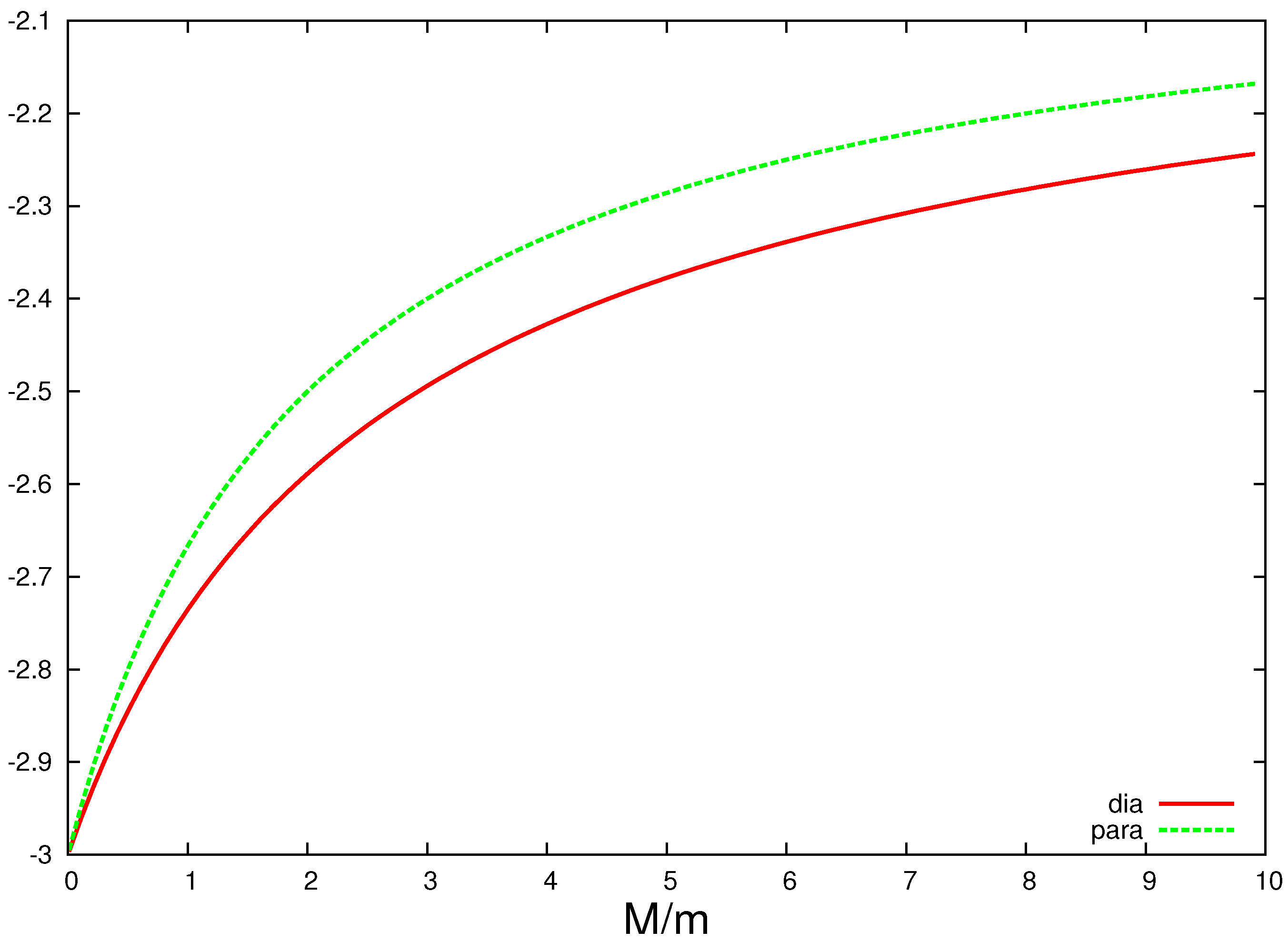

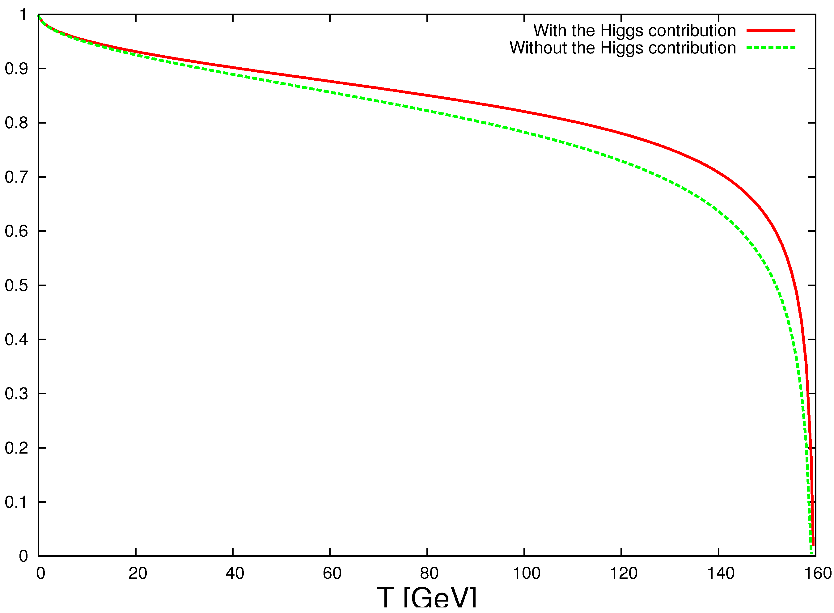
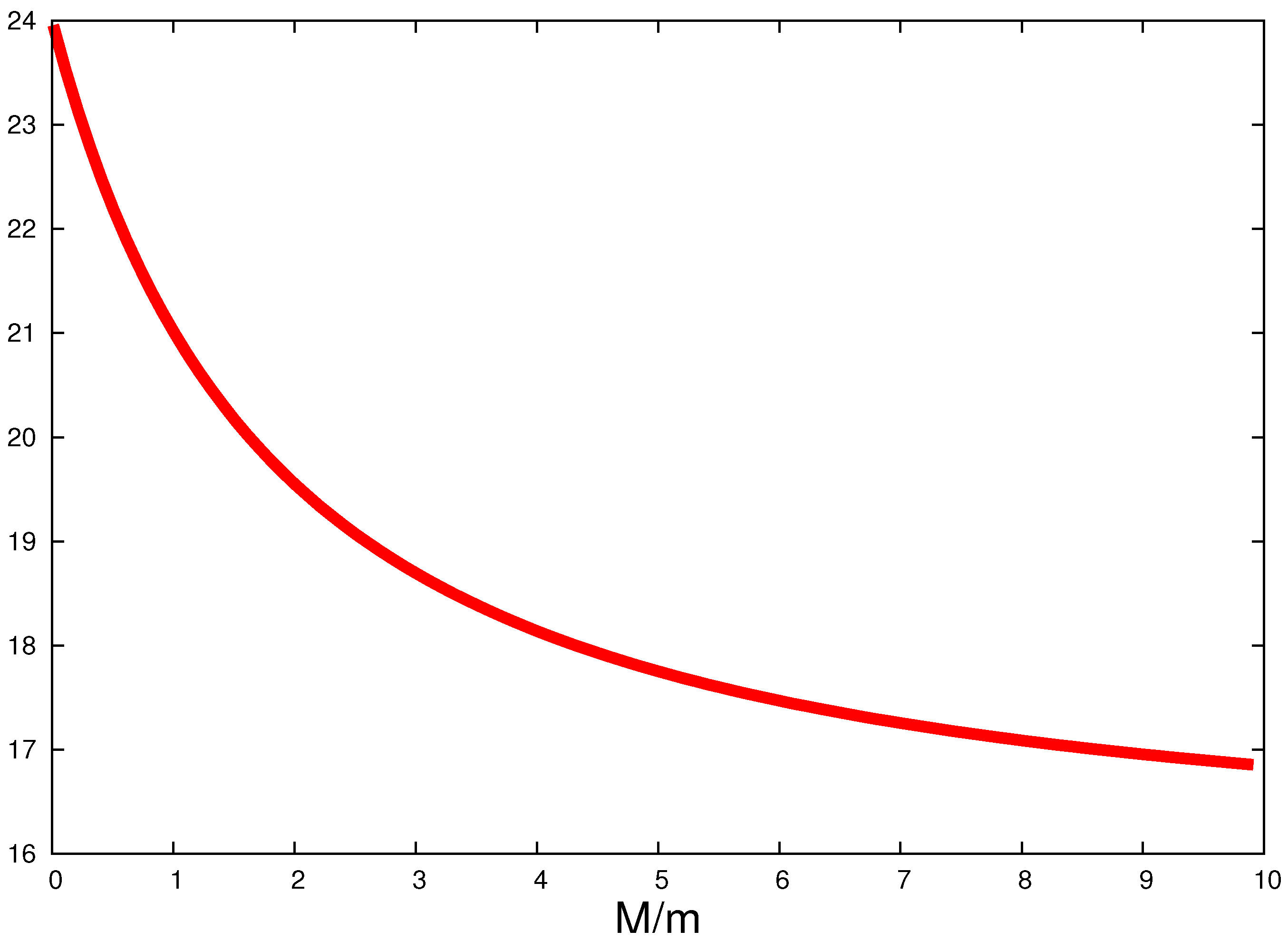