Quantum–Classical Diagnostics and Bohmian Inequivalence for Higher Time-Derivative Hamiltonians

Abstract

We develop a Bohmian analysis of a two-dimensional ghost Hamiltonian and its mapping to the degenerate Pais-Uhlenbeck model. Using Gaussian wavepackets, we derive the corresponding guidance equations, the centre and width evolution, and the quantum potential. We use these quantities to characterise bounded, quasi-semiclassical, spiral, and runaway regimes. The Bohmian trajectories provide a direct dynamical diagnostic of coherence, packet deformation, and quantum–classical separation. We then compare a bi-Hamiltonian pair consisting of the ghost Hamiltonian and a classically equivalent alternative formulation. While the two descriptions produce identical classical trajectories, they lead to different Bohmian trajectories and different quantum potentials evaluated along those trajectories. This demonstrates that classical equivalence need not extend to Bohmian quantum dynamics and identifies a concrete quantum ambiguity in the degenerate higher-derivative system.

1. Introduction

Higher time-derivative theories (HTDTs) arise naturally in a wide range of physical contexts, including effective field theory [1], modified gravity [2,3,4], regularisation schemes [2,5], and attempts at ultraviolet completion [6,7,8]. Their main structural difficulty is well known: in non-degenerate settings, higher derivatives generically lead to Ostrogradsky instabilities [9,10,11,12,13], which manifest themselves classically through unbounded Hamiltonians and quantum-mechanically through ghost sectors, unbounded spectra, or non-normalisable states [14,15]. Determining whether such systems admit a meaningful quantum interpretation, and in what sense different Hamiltonian formulations should be regarded as equivalent, remains a central open question.

A particularly useful laboratory for these issues is provided by the Pais-Uhlenbeck (PU) oscillator [16] and its equivalent ghost Hamiltonian formulations [14,15]. In these systems one encounters, already at the level of exactly solvable models, the characteristic tension between bounded spectra and normalisability, as well as the possibility of different Hamiltonian descriptions generating the same classical equations of motion [14,15]. This makes them especially suitable for probing the distinction between classical equivalence and quantum equivalence. In the degenerate case, where the two PU frequencies coincide, the dynamics becomes particularly subtle: the classical motion develops Jordan-block features and runaway secular terms, while the quantum theory exhibits additional ambiguities and a nontrivial algebraic structure with hidden symmetries [17].

In this work we analyse these systems from the viewpoint of Bohmian mechanics [18,19,20,21,22]. Rather than focusing only on spectral properties, we study the actual trajectory flow generated by the wavefunction. This has two advantages. First, it provides a direct dynamical diagnostic of the extent to which a given wavepacket behaves semiclassically, remains coherent, or develops strong quantum distortions. Second, it allows one to compare classically equivalent Hamiltonian formulations at the level of their pilot-wave dynamics, thereby revealing quantum differences that are not visible in the classical equations alone.

We restrict attention to real-time Bohmian evolution. This should be distinguished from complex [22] and imaginary-time trajectory formulations [23]. The former were used to identify coherent states in non-Hermitian systems and the latter for eigenvalue problems and quantum statistical mechanics. The question addressed here is different: we ask whether classically equivalent Hamiltonian representations generate equivalent real-time Bohmian guidance flows.

We begin with a two-dimensional ghost Hamiltonian and construct Gaussian wavepackets whose centres follow the classical motion while their widths evolve according to a Riccati equation. The corresponding Bohmian trajectories are then compared with classical trajectories and with the motion of the Gaussian centre. This leads to a set of trajectory-based diagnostics, including the internal deviation from the centre, the quantum–classical separation, and the quantum potential evaluated along the Bohmian paths. These diagnostics allow us to distinguish several qualitatively different regimes, ranging from rigid transport and quasi-semiclassical motion to unstable spiral behaviour, critical runaway motion, and non-normalisable Gaussian sectors.

A second objective is to connect these diagnostics to HTDTs more directly. The ghost Hamiltonian considered here is related to a higher time-derivative model through the standard reduction to first-order form. This allows us not merely to reinterpret the ghost dynamics, but to formulate a corresponding Bohmian diagnostic framework for the associated higher time-derivative system.

The most striking effect appears in the bi-Hamiltonian setting. In addition to the ghost Hamiltonian $H_g$, the same degenerate classical dynamics admits a second Hamiltonian description $H_2$ with a different kinetic structure [15,17]. Although the two Hamiltonians generate identical classical trajectories, we find that their Bohmian trajectories and trajectory-evaluated quantum potentials differ. This provides a concrete example of a quantum ambiguity hidden behind classical equivalence: the classical vector field is the same, but the pilot-wave dynamics is not.

Our paper is organised as follows: In Section 2 we formulate the Bohmian dynamics of the two-dimensional ghost Hamiltonian and develop its interpretation in the corresponding higher time-derivative setting obtained by reduction to first-order form. In Section 3 we analyse the Gaussian wavepacket dynamics and use Bohmian diagnostics to classify several dynamical regimes. In Section 4 we turn to the bi-Hamiltonian structure and show that classically equivalent Hamiltonians can lead to inequivalent Bohmian flows. Section 5 contains our conclusions.

2. Bohmian Dynamics for a 2D Ghost Hamiltonian and HTDTs

2.1. From the Schrödinger Equation to Quantum Potentials

We consider a two-dimensional quantum system with configuration variables $q=(x,y)$ and Hamiltonian operator of the form

$$\widehat{H}={\displaystyle \frac{1}{2}}{\widehat{p}}_i{G}^{ij}{\widehat{p}}_j+V(x,y),i,j\in \{x,y\},$$

(1)

where $G^{ij}$ is a constant symmetric matrix, not necessarily positive definite. In the coordinate representation ${\widehat{p}}_i=-i\hslash {\partial }_i$, the Schrödinger equation reads

$$i\hslash {\partial }_t\psi (x,y,t)=\left[-{\displaystyle \frac{{\hslash }^2}{2}}{\partial }_i\left(G^{ij}{\partial }_j\right)+V(x,y)\right]\psi (x,y,t).$$

(2)

We write the wavefunction in polar form

$$\psi (x,y,t)=R(x,y,t)e^{iS(x,y,t)/\hslash },R\ge 0,$$

(3)

with real amplitude R and real phase S. The decomposition is understood locally on regions where $R(q,t)\ne 0$. At nodal points the phase is not uniquely defined and the Bohmian velocity field may become singular. The equivalence with the Schrödinger equation should therefore be interpreted on nodal-free domains, or distributionally with suitable matching conditions across nodal sets. The Gaussian wavepackets used below are node-free in the regimes considered.

Substituting this Ansatz into Equation (2) and separating real and imaginary parts yields two equations. The imaginary part gives the continuity equation

$${\partial }_t\left(R^2\right)+{\partial }_i\left(R^2{G}^{ij}{\partial }_{j}S\right)=0.$$

(4)

This equation is the continuity equation for the density $\rho$ with associated current j,

$$\rho ={\left|\psi \right|}^2=R^2,\mathrm{and}{j}^i=R^2{G}^{ij}{\partial }_{j}S.$$

(5)

In turn, the real part yields the quantum Hamilton–Jacobi equation

$${\partial }_{t}S+{\displaystyle \frac{1}{2}}{\partial }_{i}S{G}^{ij}{\partial }_{j}S+V+Q=0,$$

(6)

where the quantum potential is identified as

$$Q=-{\displaystyle \frac{{\hslash }^2}{2}}{\displaystyle \frac{1}{R}}{\partial }_i\left(G^{ij}{\partial }_{j}R\right).$$

(7)

On such nodal-free domains, Equations (4) and (6) are equivalent to the Schrödinger Equation (2). No further assumptions have been made so far.

2.2. Bohmian Guidance Law from Equivariance

In Bohmian mechanics one postulates that the configuration variables $q\left(t\right)=\left(x\right(t),y(t\left)\right)$ follow deterministic trajectories guided by the wavefunction [18,19,20,21]. Denoting the velocity field by $v(q,t)$, an ensemble of such trajectories with density $\rho (q,t)$ satisfies the transport equation

$${\partial }_t\rho +{\partial }_i\left(\rho v^i\right)=0.$$

(8)

Requiring equivariance, i.e., that $\rho (q,t)={\left|\psi (q,t)\right|}^2=R^2(q,t)$ at all times, the transport equation (Equation (8)) must coincide with the continuity equation (Equation (4)). Comparing the two equations, we identify

$$\rho v^i=j^i.$$

(9)

Using expression (5) for the current, the Bohmian velocity field is therefore

$$v^i(q,t)=G^{ij}{\partial }_{j}S(q,t).$$

(10)

Thus, the Bohmian guidance equations are

$${\dot{q}}^i\left(t\right)=G^{ij}{\partial }_{j}S\left(q\left(t\right),t\right).$$

(11)

To assess the role of quantum effects, we compare these Bohmian trajectories with the corresponding classical trajectories obtained from

$$\dot{q}={\displaystyle \frac{\partial H}{\partial p}},\dot{p}=-{\displaystyle \frac{\partial H}{\partial q}}$$

(12)

with the same initial position $q\left(0\right)$ as the Bohmian particle and its momentum chosen as $p\left(0\right)=\mathsf{\nabla }S\left(q\right(0),0)$.

It is useful to stress the sense in which the term “phase space” is used below. The Bohmian dynamics considered in this work is formulated as a configuration-space dynamics: the actual variables are the coordinates $q\left(t\right)=\left(x\right(t),y(t\left)\right)$, and their velocity is determined by the phase of the wavefunction through the guidance equation. The momentum variables enter either as classical variables in the comparison system, or through the phase gradient used to initialise the corresponding classical trajectory. Thus we do not use a coordinate-momentum quantum phase-space formulation, such as Wigner-type or semiclassical phase-space methods; see, e.g., [24,25]. When we refer to classical phase-space equivalence, we mean equivalence of the classical Hamiltonian vector fields on the coordinate-momentum phase space. The question addressed here is whether such classical equivalence is sufficient to imply equivalence of the induced configuration-space Bohmian flow.

2.3. Relation to Higher Time-Derivative Theories

The purpose of this subsection is to fix the interpretation of the two configuration variables used below. They should not be viewed as two unrelated oscillator coordinates only, but also as the enlarged first-order configuration variables obtained from a higher-derivative degree of freedom. In this reduced description, different Hamiltonian representatives may reproduce the same classical higher-derivative equation while possessing different kinetic tensors. Since the Bohmian guidance equation depends explicitly on this kinetic tensor, the reduced first-order formulation is not merely a rewriting: it determines the pilot-wave dynamics.

The connection with HTDTs is made through the standard reduction to first-order form. Starting from a higher-derivative Lagrangian

$$L(q,\dot{q},\ddot{q},\dots ),$$

(13)

one introduces auxiliary variables so that the dynamics is rewritten as an equivalent first-order system on an enlarged configuration space. In the simplest case of a second-order reduction one may take

$$Q=(q,v),v=\dot{q},$$

(14)

and formulate the corresponding Schrödinger problem in these reduced variables. The resulting Hamiltonian typically contains a ghost sector because it is linear in at least one canonical momentum, thereby inheriting the characteristic Ostrogradsky-type unboundedness.

From the Bohmian viewpoint, however, the reduced system can be treated in the same structural way as the two-dimensional ghost Hamiltonian considered above. Writing the wavefunction on the enlarged configuration space in polar form as

$$\mathsf{\Psi }(Q,t)=R(Q,t)e^{iS(Q,t)/\hslash },$$

(15)

the guidance law is again determined by the gradient of the phase $S(Q,t)$, composed with the kinetic tensor appearing in the reduced Hamiltonian. Thus the Bohmian flow provides a direct dynamical probe of the reduced higher-derivative system, allowing one to compare packet transport, spreading, and instability in a way that is sensitive to the chosen Hamiltonian representation.

This perspective is especially useful in settings where different first-order reductions or Hamiltonian representations generate the same classical equations of motion. As we shall see below, such classical equivalence need not imply Bohmian quantum equivalence, since the guidance law retains information about the specific Hamiltonian structure used in the quantisation. The trajectory-based formulation therefore provides additional information beyond the classical phase-space dynamics alone, and is particularly well suited to the analysis of higher time-derivative models with nonstandard kinetic structure.

3. Diagnostics of a Coupled Ghost Oscillator Model

We consider the two-dimensional ghost Hamiltonian with Lorentzian kinetic term introduced in [14,15],

$$H_{\mathrm{gh}}(x,y,p_x,p_y)={\displaystyle \frac{1}{2}}\left(p_x^2-p_y^2\right)+{\nu }^2{x}^2+\Omega y^2+gxy,\nu ,\Omega ,g\in \mathbb{R},$$

(16)

with corresponding Schrödinger equation

$$i\hslash {\partial }_t\psi (x,y,t)=\left[-{\displaystyle \frac{{\hslash }^2}{2}}\left({\partial }_x^2-{\partial }_y^2\right)+V_{\mathrm{gh}}(x,y)\right]\psi (x,y,t),$$

(17)

where

$$V_{\mathrm{gh}}(x,y)={\displaystyle \frac{1}{2}}{q}^{⊺}Cq,C=\left(\begin{array}{cc}2{\nu }^2& g\\ g& 2\Omega \end{array}\right).$$

(18)

To probe nontrivial Bohmian dynamics, we work with Gaussian wavepackets rather than stationary eigenstates.

3.1. Gaussian Wavepackets and Diagnostic Quantities

We begin with a Gaussian wavepacket of the form

$${\psi }_g(q,t)=\mathcal{N}\left(t\right)exp\left[-{\displaystyle \frac{1}{2\hslash }}{(q-q_c)}^{⊺}(A+iB)(q-q_c)+{\displaystyle \frac{i}{\hslash }}{p}_c·(q-q_c)+{\displaystyle \frac{i}{\hslash }}\theta \left(t\right)\right],$$

(19)

where $A\left(t\right)$ and $B\left(t\right)$ are real symmetric matrices, $q_c\left(t\right)$ is the configuration-space centre, and $p_c\left(t\right)$ the corresponding central momentum. We choose the Gaussian to be centred at a phase-space point $(q_c\left(t\right),p_c\left(t\right))$. These variables are not independent new degrees of freedom. They denote the centre of the packet and its conjugate central momentum. For a quadratic Hamiltonian, substitution into the Schrödinger equation forces $(q_c,p_c)$ to satisfy the corresponding classical Hamilton equations. Thus $q_c\left(t\right)$ is the classical trajectory traced by the packet centre, with initial data specified in the numerical examples.

Substituting (19) into (17) yields

$${\dot{q}}_c=G{p}_c,{\dot{p}}_c=-C{q}_c,$$

(20)

together with the Riccati equation

$$\dot{K}=-i(KGK-C),K=A+iB,$$

(21)

together with evolution equations for $\theta \left(t\right)$ and $\mathcal{N}\left(t\right)$, which determine the overall phase and normalisation but do not affect the trajectory analysis directly. Since (20) coincides with the classical equations of motion,

$$\dot{q}=Gp,\dot{p}=-Cq,$$

(22)

the centre of the Gaussian packet follows the classical trajectory exactly, as expected for quadratic Hamiltonians; see, e.g., [26,27].

Factorising ${\psi }_g$ in (19) into the polar form (3) using

$$R\propto exp\left[-{\displaystyle \frac{1}{2\hslash }}{(q-q_c)}^{⊺}A(q-q_c)\right],S=-{\displaystyle \frac{1}{2}}{(q-q_c)}^{⊺}B(q-q_c)+p_c·(q-q_c)+\theta ,$$

(23)

we obtain with (18) the Bohmian guidance law

$$\dot{q}=G\mathsf{\nabla }S,\mathsf{\nabla }S(q,t)=p_c-B(q-q_c),$$

(24)

together with the quantum potential

$$Q(q,t)=-{\displaystyle \frac{1}{2}}{(q-q_c)}^{⊺}AGA(q-q_c)+{\displaystyle \frac{\hslash }{2}}\mathrm{Tr}\left(GA\right).$$

(25)

We distinguish three configuration-space trajectories. The first is the Gaussian centre $q_c\left(t\right)$, determined by Equation (20). The second is a Bohmian trajectory $q_B\left(t\right)$, obtained by integrating the guidance Equation (24) with initial position sampled from ${\left|\psi (q,0)\right|}^2$. The third is the associated classical trajectory $q_{\mathrm{cl}}\left(t\right)$, obtained from Equation (22) with the same initial position as $q_B\left(0\right)$ and with initial momentum $p_{\mathrm{cl}}\left(0\right)=\mathsf{\nabla }S(q_B\left(0\right),0)$. Thus $q_c\left(t\right)$ is a single centre trajectory, while $q_{\mathrm{cl}}\left(t\right)$ is the member of the classical ensemble corresponding to the same initial data as a given Bohmian path.

It is convenient to introduce the deviation from the packet centre,

$$u\left(t\right):=q_B\left(t\right)-q_c\left(t\right),$$

(26)

and the quantum–classical separation,

$$\mathsf{\Delta }\left(t\right):=q_B\left(t\right)-q_{\mathrm{cl}}\left(t\right).$$

(27)

Using (24) and (20), the deviation satisfies the first-order equation

$$\dot{u}=-GBu.$$

(28)

Thus the internal Bohmian flow is controlled by the matrix

$$M\left(t\right):=-GB\left(t\right),$$

(29)

whose symmetric part

$$S_M\left(t\right):={\displaystyle \frac{1}{2}}\left(M\left(t\right)+M^{⊺}\left(t\right)\right)$$

(30)

controls the instantaneous growth or decay of the deviation $u\left(t\right)$. This is seen from

$${\displaystyle \frac{d}{dt}}{\parallel u\left(t\right)\parallel }^2={\displaystyle \frac{d}{dt}}\left(u^{⊺}u\right)={\dot{u}}^{⊺}u+u^{⊺}\dot{u}=u^{⊺}\left(M^{⊺}+M\right)u=2u^{⊺}{S}_M\left(t\right)u,$$

(31)

so that positive eigenvalues of $S_M\left(t\right)$ correspond to locally expanding directions in the Bohmian flow, while negative eigenvalues correspond to contracting directions. The antisymmetric part of $M\left(t\right)$ contributes only to the rotational part of the motion and does not directly change the magnitude of $u\left(t\right)$.

Differentiating (28) and using (21) gives the equivalent second-order equation

$$\ddot{u}=-G\Lambda u,\Lambda :=C-AGA.$$

(32)

The matrix $\Lambda$ measures the mismatch between the classical curvature C and the quantum curvature $AGA$. When $\Lambda =0$, the internal acceleration vanishes and the packet undergoes rigid transport, and when $\Lambda \ne 0$, Bohmian trajectories deform relative to the centre.

The diagnostic matrix $\Lambda$ is tied to the Gaussian ansatz, since it uses the width matrix $A\left(t\right)$ of the packet. It should therefore be understood as a Gaussian diagnostic of the competition between classical curvature and quantum curvature, rather than as a state-independent object.

These equations provide a compact classification criterion. Since the Bohmian trajectory can be written as $q_B\left(t\right)=q_c\left(t\right)+u\left(t\right)$, bounded motion requires control of both the packet centre and the internal deviation, as well as admissibility of the Gaussian state itself. First, the packet must remain normalisable, which in the present parametrisation means that the amplitude matrix A remains positive definite. Second, the centre trajectory $q_c\left(t\right)$ must stay bounded, since otherwise the full Bohmian motion inherits the runaway of the packet centre. Third, the internal flow generated by $-GB$ must avoid sustained expanding directions, so that the deviation $u\left(t\right)$ does not grow secularly. Failure of these three conditions leads respectively to non-normalisability of the state, drift-induced runaway of the full trajectory, or internally amplified Bohmian instability.

A useful structural observation is that exact cancellation, $\Lambda =0$, can occur only for non-confining saddle-type potentials. Indeed, $\Lambda =0$ implies $C=AGA$, and hence

$$det\left(AGA\right)=det\left(G\right)det{\left(A\right)}^2=-det{\left(A\right)}^2<0,$$

(33)

so $AGA$, and therefore C, must be indefinite:

$$detC=4{\nu }^2\Omega -g^2<0.$$

(34)

Thus, if C is positive definite, one necessarily has $\Lambda \ne 0$, so no Gaussian state can exactly cancel the classical curvature. In this sense, the mixed signature of G obstructs the usual coherent-state cancellation mechanism familiar from positive-definite systems.

In the numerical examples below we compare three families of trajectories: the classical ensemble obtained from (22), the Gaussian centre determined by (20), and the Bohmian ensemble obtained from (24). For the ensemble plots, the initial positions are sampled from the initial density ${\left|\psi (q,0)\right|}^2$, while the classical initial momenta are chosen from the initial phase gradient $p\left(0\right)=\mathsf{\nabla }S(q,0)$.

In the discussion below, boundedness or growth of $u\left(t\right)$ is interpreted through the internal flow $\dot{u}=-GBu$, while the behaviour of $\Lambda \left(t\right)$ indicates whether the Bohmian dynamics remains close to the rigid-transport limit or develops significant curvature-driven deformation.

3.1.1. Rigid-Transport Regime

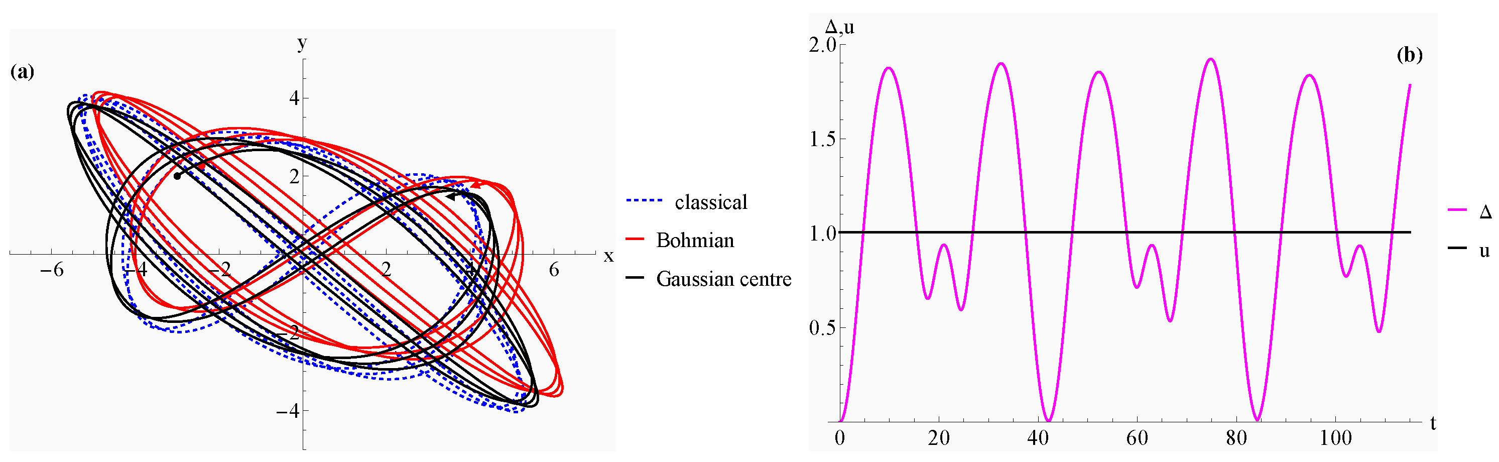
We begin with a regime in which the curvature mismatch $\Lambda \left(t\right)$ vanishes exactly or remains sufficiently small over the time interval considered that the internal acceleration in (32) is negligible. The results for this regime are shown in Figure 1.

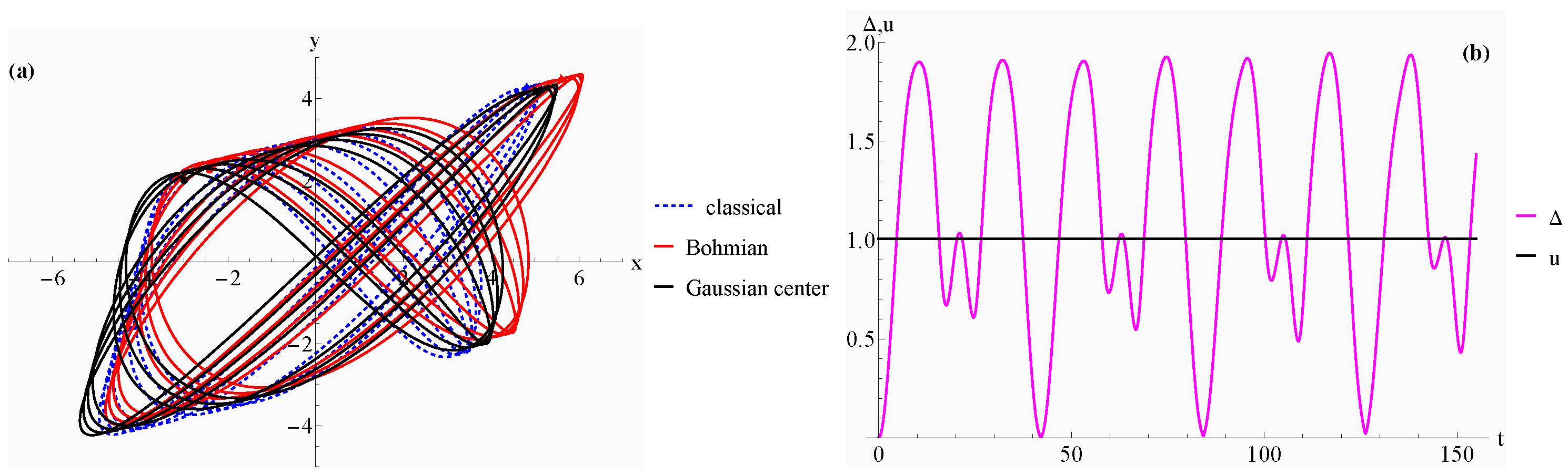
Panel (a) shows that the classical ensemble, the Bohmian ensemble, and the Gaussian centre all remain bounded and follow closely related loop-like trajectories. Panel (b) shows that the internal deviation $u\left(t\right)$ remains approximately constant, while the quantum–classical separation $\mathsf{\Delta }\left(t\right)$ exhibits only bounded oscillations. As explained in Section 3.1, this indicates that the internal flow generated by $-GB$ does not develop sustained expanding directions, and that the curvature mismatch is too weak to produce secular growth through (32). The packet is therefore transported with little internal deformation, so this regime is naturally interpreted as coherent or near-coherent rigid transport.

3.1.2. The Quasi-Semiclassical Regime $\Lambda \ne 0$

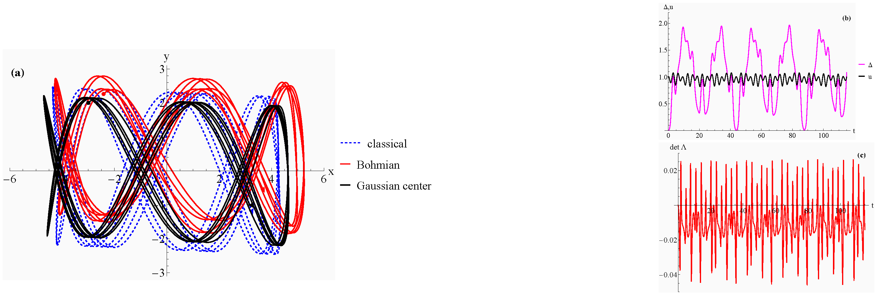
We next consider a regime in which $\Lambda \left(t\right)\ne 0$, but remains bounded and oscillatory. The corresponding trajectories are shown in Figure 2, obtained by varying only the frequency parameter $\Omega$ relative to the rigid-transport case.

Panel (a) shows that the classical ensemble, the Gaussian centre, and the Bohmian ensemble all remain bounded. Panel (b) confirms that neither the internal deviation $u\left(t\right)$ nor the quantum–classical separation $\mathsf{\Delta }\left(t\right)$ develop secular growth. Panel (c) shows that $det\Lambda \left(t\right)$ fluctuates about zero rather than remaining close to zero, so the packet is no longer in the strict rigid-transport limit. Nevertheless, these oscillations do not translate into persistent expanding directions in the internal Bohmian flow, and the resulting motion remains bounded despite the non-vanishing curvature mismatch. This regime is therefore no longer coherent in the strict $\Lambda =0$ sense, but remains quasi-semiclassical.

In this sense, the present Bohmian analysis extends the classical observations of [28,29,30] to the quantum domain. Those works showed that ghost degrees of freedom need not lead to runaway instabilities at the classical level when the coupled system is suitably structured. Here we find an analogous phenomenon for Gaussian Bohmian dynamics: despite the indefinite kinetic structure, both the packet centre and the Bohmian ensemble can remain bounded, with the bounded regime characterised by controlled curvature mismatch and the absence of persistent expansion in the internal flow.

3.1.3. The Unstable Spiral Regime

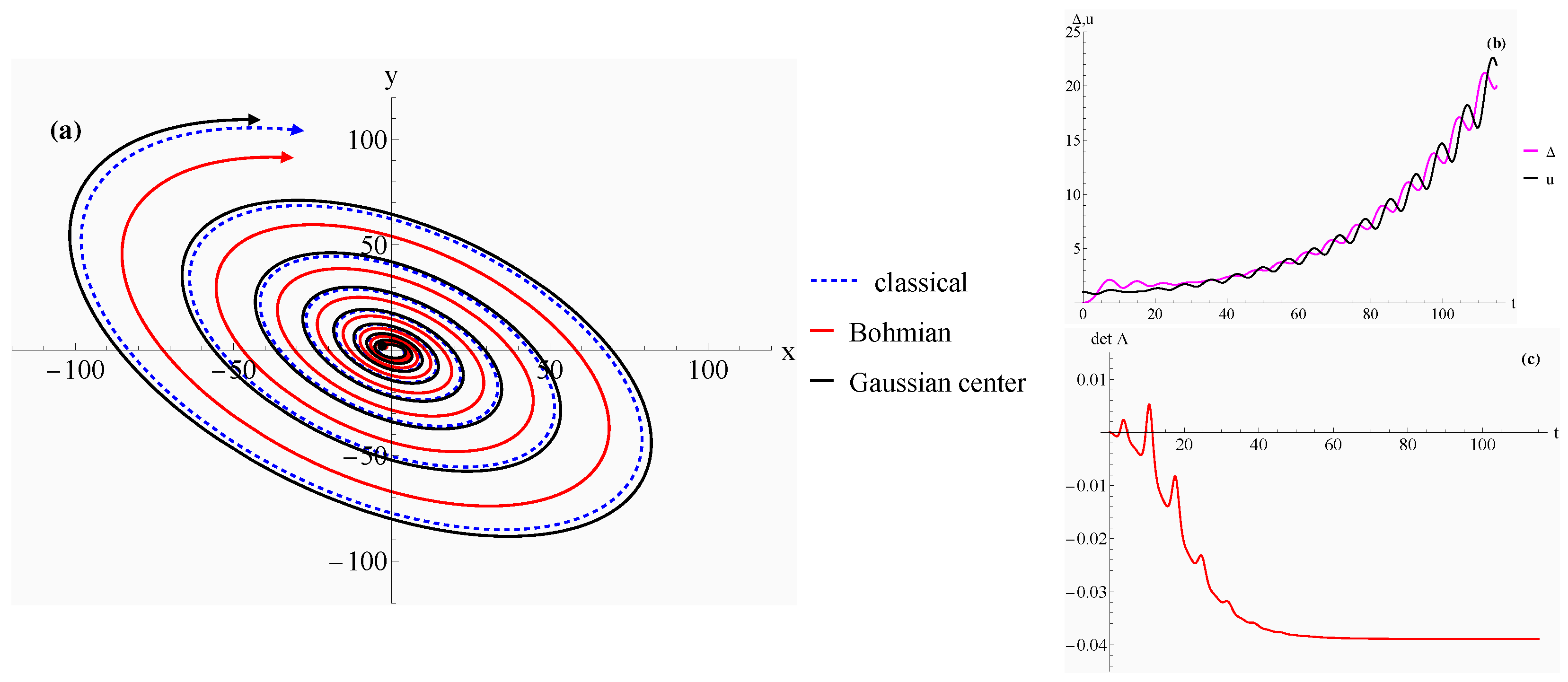
In the unstable spiral regime, the linearised centre dynamics possesses complex-conjugate eigenvalues with a positive real part, so the centre motion is already unbounded. The resulting trajectories are shown in Figure 3.

Panel (a) shows that the classical ensemble, the Gaussian centre, and the Bohmian ensemble all spiral outward with increasing amplitude. Panel (b) indicates that both the internal deviation $u\left(t\right)$ and the quantum–classical separation $\mathsf{\Delta }\left(t\right)$ grow in time, so the Bohmian flow not only follows the unstable centre motion but also develops increasing separation relative to both the packet centre and the corresponding classical trajectories. Panel (c), through the nontrivial evolution of $det\Lambda \left(t\right)$, shows that the curvature mismatch remains dynamically active throughout the spiralling phase. In terms of the diagnostics introduced in Section 3.1, this regime combines unstable centre motion with expanding behaviour in the internal flow, leading to runaway dynamics with a rotational component.

3.1.4. The Critical Regime

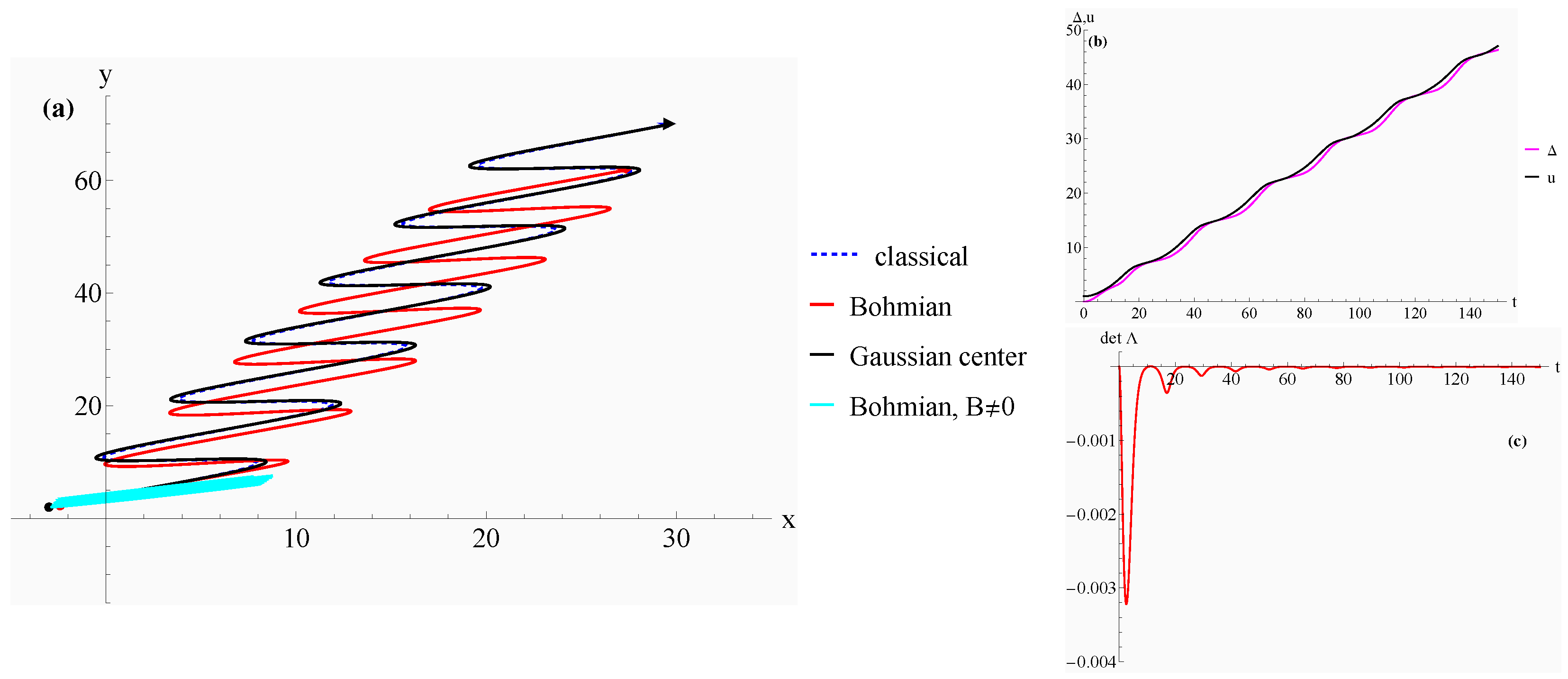
We next explore the critical regime in which the potential curvature matrix becomes degenerate, $detC=0$, while the internal curvature remains nonzero. At this point the system loses one restoring direction, so the Gaussian centre is no longer confined. The resulting trajectories are shown in Figure 4.

Panel (a) shows that all three trajectory families become unbounded. Panel (b) demonstrates that both the internal deviation $u\left(t\right)$ and the quantum–classical separation $\mathsf{\Delta }\left(t\right)$ now grow rather than oscillate, signalling the breakdown of bounded transport. Panel (c) shows that $det\Lambda \left(t\right)$ remains nonzero, so the curvature mismatch persists throughout the evolution and the dynamics does not approach the rigid-transport limit. The Bohmian trajectories typically diverge somewhat more slowly than the classical ones, especially when an initial chirp is included, but this only moderates the instability rather than removing it. According to the criteria established in Section 3.1, the critical case therefore marks the transition from bounded motion to runaway behaviour.

3.1.5. Non-Normalisable Initial Wavepacket

In models with ghost sectors of the type studied here, quantisation naturally produces multiple sectors with distinct spectral and localisation properties. As discussed in [14,15], some sectors exhibit spectra bounded from below but correspond to eigenfunctions that are not square-integrable. While such non-normalisable states are typically excluded in standard quantum mechanics because they do not belong to the Hilbert space $L^2\left({\mathbb{R}}^n\right)$, they can nevertheless be useful as formal test functions or asymptotic approximations, e.g., plane waves in scattering theory, and still generate well-defined Bohmian velocity fields [31]. Bohmian mechanics only requires a differentiable complex wavefunction to define a velocity field according to (11) without requiring a strictly normalisable probability density [18,19].

To investigate this possibility, we choose the initial spread matrix $A\left(0\right)$ so that its real symmetric part has indefinite sign, yielding a non-normalisable Gaussian packet, while retaining the rigid-transport conditions on the potential. The resulting trajectories are shown in Figure 5.

Panel (a) shows that the classical ensemble, the Bohmian ensemble, and the Gaussian centre continue to trace bounded orbits with qualitative features similar to those of the normalisable rigid-transport regime. Panel (b) shows that the internal deviation $u\left(t\right)$ remains approximately constant while $\mathsf{\Delta }\left(t\right)$ oscillates in a bounded manner. In the terminology of Section 3.1, the internal flow therefore remains non-expanding, even though the state fails the normalisability condition required for a physical Gaussian packet. This suggests that the phase-curvature cancellation mechanism underlying rigid transport is largely insensitive to square-integrability, although the resulting state should be regarded only as a diagnostic probe rather than a physical $L^2$ state.

The different cases studied above are summarised in

Table 1. Summary of the dynamical regimes studied in Section 3. Here $A\left(t\right)$ controls normalisability, $B\left(t\right)$ the local Bohmian flow, and $\Lambda \left(t\right)=C-AGA$ the curvature mismatch.

Regime	Conditions	Bohmian Behaviour	Interpretation
Rigid transport	$A\left(t\right)>0$, $\Lambda \left(t\right)\approx 0$ or $\parallel \Lambda \left(t\right)\parallel \ll 1$	$q_c\left(t\right)$ bounded; $u\left(t\right)$ and $\mathsf{\Delta }\left(t\right)$ remain bounded	coherent or near-coherent transport
Quasi-semiclassical	$A\left(t\right)>0$, $\Lambda \left(t\right)\ne 0$ but bounded	bounded centre motion with oscillatory internal deformation	breathing/shearing packet without secular growth
Spiral instability	$A\left(t\right)>0$ initially; expanding directions in $-GB\left(t\right)$	rotational flow with growing $u\left(t\right)$ and $\mathsf{\Delta }\left(t\right)$	spiral instability with quantum deformation
Critical runaway	$detC=0$, $\Lambda \left(t\right)\ne 0$	marginal behaviour followed by linear or accelerated growth	transition to runaway motion
Non-normalisable sector	$A\left(t\right)$ loses positive definiteness	formal Bohmian flow may persist	diagnostic only, not a physical $L^2$ state

, which organises the numerical results according to normalisability, centre dynamics, and internal Bohmian stability.

We stress that the non-normalisable Gaussian considered in this subsection is not used as a physical probability density and is not intended to define a normalisable quantum state in $L^2\left({\mathbb{R}}^2\right)$. Its role is diagnostic: it probes whether the guidance field and the rigid-transport mechanism persist at the formal level in a sector analogous to the non-square-integrable sectors encountered in ghost quantisation. The conclusions drawn from this example should therefore be read as statements about the structure of the velocity field, not as claims about physical normalisable wavepacket evolution.

4. Quantum Ambiguities

As discussed in the literature on the PU model, the ghost Hamiltonian formulation admits a bi-Hamiltonian partner that generates the same classical flow, while leading to a different quantum realisation; see in particular [15], and also the discussion of the hidden symmetry structure at the degenerate point in [17]. In this section we use the Bohmian framework to analyse this ambiguity dynamically.

Following [17], dropping for convenience the overall factor $1/2$ in the ghost Hamiltonian, we consider the pair

$$H_g(x,y,p_x,p_y)=p_x^2-p_y^2+{\nu }^2{x}^2+\Omega y^2-({\nu }^2+\Omega )xy,$$

(35)

and

$$\begin{array}{c}\hfill H_2={\displaystyle \frac{1}{2\sqrt{2}}}\left[{\displaystyle \frac{{\nu }^2-3\Omega }{{\nu }^2-\Omega }}{p}_x^2-2{\displaystyle \frac{{\nu }^2+\Omega }{{\nu }^2-\Omega }}{p}_x{p}_y+{\displaystyle \frac{\Omega -3{\nu }^2}{{\nu }^2-\Omega }}{p}_y^2+{\displaystyle \frac{1}{2}}\left(3{\nu }^2-\Omega \right)x^2-\left({\nu }^2+\Omega \right)xy\right.\hfill \\ \hfill \left.+{\displaystyle \frac{1}{2}}\left(3\Omega -{\nu }^2\right)y^2\right]\end{array}$$

(36)

together with the Poisson tensors

$$J_g=\left(\begin{array}{cccc}0& 0& 1& 0\\ 0& 0& 0& 1\\ -1& 0& 0& 0\\ 0& -1& 0& 0\end{array}\right),J_2={\displaystyle \frac{1}{\sqrt{2}\left({\nu }^2-\Omega \right)}}\left(\begin{array}{cccc}0& 0& 3{\nu }^2-\Omega & -{\nu }^2-\Omega \\ 0& 0& {\nu }^2+\Omega & {\nu }^2-3\Omega \\ \Omega -3{\nu }^2& -{\nu }^2-\Omega & 0& 0\\ {\nu }^2+\Omega & 3\Omega -{\nu }^2& 0& 0\end{array}\right).$$

(37)

These two Hamiltonian descriptions are classically equivalent in the sense that they generate the same phase-space vector field

$$\dot{z}=J_g\mathsf{\nabla }{H}_g=J_2\mathsf{\nabla }{H}_2,z=(x,y,p_x,p_y).$$

(38)

The equality in Equation (38) is a statement about the classical Hamiltonian vector field on the usual coordinate-momentum phase space. It should not be confused with a quantum phase-space formulation of the dynamics. In the Bohmian formulation used here, the quantum dynamics is represented by a configuration-space guidance law. The key point is that two Hamiltonian representations may define the same classical phase-space flow while inducing different Bohmian velocity fields on configuration space, because the latter depend explicitly on the kinetic tensor entering the quantised Hamiltonian.

Thus any difference found below is not classical in origin, but arises from the representation dependence of the corresponding Bohmian quantum theory.

This becomes explicit once the Gaussian ansatz (19) is inserted into the guidance law. Although the two Hamiltonians generate the same classical equations of motion, they do so with different kinetic tensors, and these enter directly into the Bohmian velocity field. Writing the momentum-sector quadratic form as

$$H_{\alpha }^{\mathrm{kin}}=p^{⊺}{G}_{\alpha }p,\alpha \in \{g,2\},$$

(39)

the corresponding tensors are

$$G_g=\left(\begin{array}{cc}1& 0\\ 0& -1\end{array}\right),G_2={\displaystyle \frac{1}{2\sqrt{2}({\nu }^2-\Omega )}}\left(\begin{array}{cc}{\nu }^2-3\Omega & -({\nu }^2+\Omega )\\ -({\nu }^2+\Omega )& \Omega -3{\nu }^2\end{array}\right).$$

(40)

Hence the Bohmian trajectories are obtained from

$${\dot{q}}_{B,\alpha }\left(t\right)=G_{\alpha }\mathsf{\nabla }{S}_{\alpha }(q,t),\alpha \in \{g,2\},$$

(41)

with the same initial positions sampled from the same initial packet, but with the guidance law determined in each case by the corresponding kinetic tensor $G_{\alpha }$. Even when the initial phase profile is chosen identically, the subsequent Bohmian evolution differs because the velocity field depends explicitly on $G_{\alpha }$. This is the precise origin of the representation dependence studied in this section.

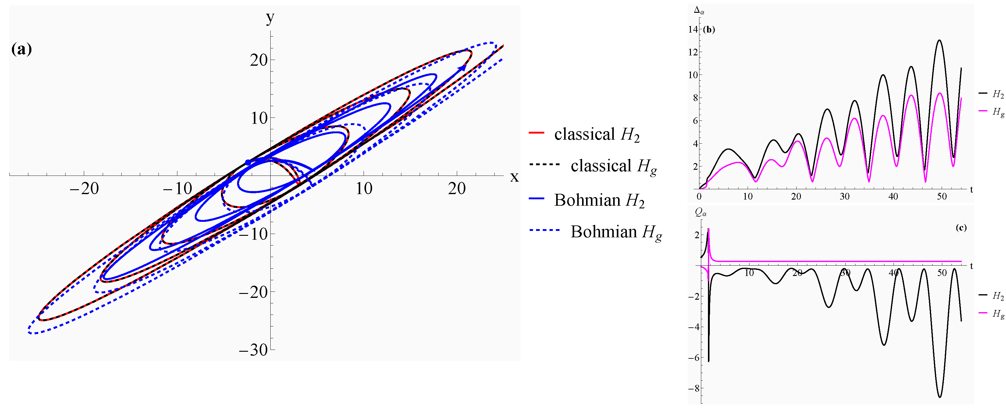
The resulting configuration-space trajectories are displayed in Figure 6a. The classical ensembles generated by $H_g$ and $H_2$ coincide, in agreement with (38). By contrast, the Bohmian ensembles do not coincide. In both formulations the motion exhibits the same outward-spiralling runaway behaviour, as expected at the degenerate point of the PU oscillator, but the detailed Bohmian flow is visibly representation-dependent. Thus the common classical instability is dressed by different quantum corrections in the two Hamiltonian descriptions.

A convenient way to quantify this effect is through the quantum–classical separation

$${\mathsf{\Delta }}_{\alpha }\left(t\right):=q_{B,\alpha }\left(t\right)-q_{\mathrm{cl}}\left(t\right),\alpha \in \{g,2\},$$

(42)

where $q_{\mathrm{cl}}\left(t\right)$ denotes the common classical trajectory with the same initial position and initial momentum fixed from the initial phase gradient. Figure 6b shows the corresponding norms. In both cases the separation grows along the runaway motion, so the quantum correction does not remain a bounded perturbation of the classical orbit. Moreover, the growth is systematically stronger for $H_2$ than for $H_g$, showing that the second Hamiltonian representation induces a larger quantum departure from the same classical background.

Further insight is obtained from the quantum potential. For the Gaussian wavepacket considered here, the expression derived in (25) reads

$$Q_{\alpha }(q,t)=-{\displaystyle \frac{1}{2}}{\left(q-q_{c,\alpha }\left(t\right)\right)}^{⊺}{A}_{\alpha }\left(t\right)G_{\alpha }{A}_{\alpha }\left(t\right)\left(q-q_{c,\alpha }\left(t\right)\right)+{\displaystyle \frac{\hslash }{2}}\mathrm{Tr}\left(G_{\alpha }{A}_{\alpha }\left(t\right)\right),\alpha \in \{g,2\}.$$

(43)

It is important to distinguish the field $Q_{\alpha }(q,t)$ on configuration space from the quantity actually shown in Figure 6c, namely the quantum potential evaluated along the Bohmian trajectory

$$Q_{B,\alpha }\left(t\right):=Q_{\alpha }\left(q_{B,\alpha }\left(t\right),t\right).$$

(44)

Because $Q_{\alpha }$ depends explicitly on the kinetic tensor $G_{\alpha }$, the two representations need not yield the same quantum potential even though they share the same classical flow. This is exactly what is seen in Figure 6c. In the $H_g$ case, $Q_{B,g}\left(t\right)$ exhibits only a short initial transient before settling to an almost constant value. By contrast, in the $H_2$ case the quantum potential remains strongly time-dependent and develops increasingly large oscillatory excursions. The two formulations therefore share the same classical runaway background, but differ significantly in the effective quantum force acting along the Bohmian trajectories.

Taken together, panels (a)–(c) of Figure 6 provide a clear dynamical manifestation of the quantisation ambiguity already identified algebraically in [15,17]. The pair $(H_g,J_g)$ and $(H_2,J_2)$ is classically equivalent, but the associated Bohmian theories are not. The ambiguity is therefore genuinely quantum. It is invisible at the level of the classical phase-space vector field, but becomes manifest once one compares the Bohmian trajectories, the quantum–classical separation, and the quantum potential evaluated along the trajectories.

We emphasise that the inequivalence established here is a Bohmian dynamical inequivalence. It concerns the trajectory field and the quantum potential evaluated along that trajectory. We do not claim that every conventional Hilbert-space observable must necessarily distinguish the two representations without specifying an operational measurement model. In standard quantum mechanics, the comparison of two quantisations would require a statement about the Hilbert space, inner product, domain, and observable algebra. Our result is instead that classical equivalence of the phase-space vector field is not sufficient to guarantee equivalence of the corresponding pilot-wave dynamics.

We stress that the representation dependence discussed in this section is not tied to this particular Gaussian diagnostic. It follows already from the Bohmian guidance law, whose velocity field depends explicitly on the kinetic tensor of the Hamiltonian representation. For a general wavefunction $\psi =Rexp(iS/\hslash )$, two classically equivalent Hamiltonian descriptions with different kinetic tensors $G_{\alpha }$ lead to velocity fields ${\dot{q}}_{\alpha }=G_{\alpha }\mathsf{\nabla }{S}_{\alpha }$, and hence need not define the same Bohmian flow. The Gaussian ansatz makes this difference analytically and numerically transparent, but it is not the sole origin of the inequivalence.

All numerical trajectories were obtained with Mathematica’s built-in function NDSolveValue by integrating the coupled ordinary differential equations for the centre variables, the Bohmian trajectories, and the Riccati equation for the Gaussian width matrix. The Riccati equation was integrated directly for the complex matrix $K\left(t\right)=A\left(t\right)+iB\left(t\right)$, after which $A\left(t\right)=\mathrm{Re}K\left(t\right)$ and $B\left(t\right)=\mathrm{Im}K\left(t\right)$ were extracted. The integrations were performed with Mathematica’s adaptive automatic time-stepping algorithm, using Method -> Automatic, AccuracyGoal -> Automatic, andPrecisionGoal -> Automatic. We set $MaxExtra Precision = 50. For the centre evolution we used MaxStepFraction -> 1/200, while for the Riccati equation, Bohmian trajectories, and associated classical trajectories we used MaxStepFraction -> 1/400. In the unstable spiral and critical regimes we checked numerical stability by reducing the maximal step size and repeating the integrations; the displayed trajectories and diagnostic curves did not change on the scale shown in the figures. The plotted curves are restricted to time intervals for which these convergence checks remained stable.

5. Conclusions

We analysed the Bohmian dynamics of a two-dimensional ghost Hamiltonian and its relation to HTDTs, with particular emphasis on Gaussian states and on the bi-Hamiltonian structure of the degenerate PU model. Our aim was not only to describe the corresponding quantum trajectories, but to test whether a trajectory-based formulation can reveal features that are less transparent at the level of spectral data or classical equations of motion alone.

For Gaussian wavepackets, the Bohmian formulation leads naturally to a set of dynamical diagnostics. The packet centre follows the classical trajectory exactly, while the internal Bohmian deformation is governed by the phase-curvature matrix B and, at second order, by the curvature-mismatch matrix $\Lambda$. This makes it possible to distinguish bounded rigid transport, quasi-semiclassical deformation, unstable spiral motion, critical runaway behaviour, and non-normalisable sectors within a unified framework. In this sense, Bohmian trajectories do not merely reproduce the classical flow, but provide a direct dynamical probe of coherence, spreading, and instability.

More specifically, the bounded quasi-semiclassical regimes found here provide a Bohmian quantum extension of classical results showing that suitably coupled ghost sectors need not exhibit runaway instabilities [28,29,30]. In the present setting, this persistence of bounded motion is diagnosed through bounded centre dynamics, bounded internal deviation, and the absence of sustained expansion in the internal Bohmian flow.

A compact analytical picture also emerges from the Gaussian ansatz. The deviation $u=q-q_c$ from the packet centre satisfies the first-order equation

$$\dot{u}=-GBu,$$

(45)

and hence the local stability of the Bohmian flow is controlled by the symmetric part of the matrix $-GB$, while the second-order equation

$$\ddot{u}=-G\Lambda u$$

(46)

encodes the competition between classical and quantum curvature. Bounded Bohmian motion therefore requires three ingredients: a normalisable packet, bounded centre motion, and the absence of sustained expanding directions in the internal flow. These criteria organise the different regimes observed in our numerical analysis.

The main conceptual result of the paper is obtained in the bi-Hamiltonian setting. We showed that two Hamiltonian descriptions which generate the same classical phase-space vector field need not lead to the same Bohmian quantum theory. Although the ghost Hamiltonian $H_g$ and its classically equivalent partner $H_2$ produce identical classical trajectories, their Bohmian trajectories and trajectory-evaluated quantum potentials differ because the guidance law depends explicitly on the kinetic tensor of the chosen Hamiltonian representation. Classical equivalence is therefore too weak a criterion for Bohmian quantum equivalence.

This observation is particularly relevant for higher time-derivative systems, where reductions to first-order form and alternative Hamiltonian structures are common. Our results suggest that such formulations should not be compared solely through their classical equations or spectral properties. Trajectory-based diagnostics provide additional information about quantum transport, coherence, and instability, and may therefore serve as a useful tool in assessing competing quantisations of higher-derivative models.

We have also restricted the present analysis to continuous degrees of freedom. This is the natural setting for the higher time-derivative Hamiltonians and PU-type systems studied here. Extensions to mixed continuous/discrete systems, such as nonadiabatic molecular models or composite systems relevant to light-induced dynamics and quantum information, would require additional structure. In such cases the wavefunction has discrete components, or equivalently a matrix-valued potential structure, and the Bohmian description may involve conditional wavefunctions, component-dependent velocity fields, or additional rules for transitions between discrete sectors. It would be interesting to investigate whether the representation dependence identified here has an analogue in such mixed systems, but this lies beyond the scope of the present work.

A natural next step would be to extend the present analysis beyond single Gaussian states and to use different types of diagnostic probe functions to study interference effects, nodal structures, and their impact on Bohmian transport. We leave this question for future work.

References

1. Buchbinder, I.L. Effective Action in Quantum Gravity; Routledge: London, UK, 2017. [Google Scholar]
2. Stelle, K.S. Renormalization of higher-derivative quantum gravity. Phys. Rev. D 1977, 16, 953. [Google Scholar] [CrossRef] [Scilit]
3. Starobinsky, A.A. A new type of isotropic cosmological models without singularity. Phys. Lett. B 1980, 91, 99–102. [Google Scholar] [CrossRef] [Scilit]
4. Sotiriou, T.P.; Faraoni, V. f(R) theories of gravity. Rev. Mod. Phys. 2010, 82, 451–497. [Google Scholar] [CrossRef] [Scilit]
5. Smilga, A.V. Spontaneous generation of the Newton constant in the renormalizable gravity theory. arXiv 2014, arXiv:1406.5613. [Google Scholar]
6. Barnaby, N.; Kamran, N. Dynamics with infinitely many derivatives: The initial value problem. J. High Energy Phys. 2008, 2008, 008. [Google Scholar] [CrossRef] [Scilit]
7. Tomboulis, E. Renormalization and unitarity in higher derivative and nonlocal gravity theories. Mod. Phys. Lett. A 2015, 30, 1540005. [Google Scholar] [CrossRef] [Scilit]
8. Modesto, L.; Shapiro, I.L. Superrenormalizable quantum gravity with complex ghosts. Phys. Lett. B 2016, 755, 279–284. [Google Scholar] [CrossRef] [Scilit]
9. Ostrogradsky, M. Mémoire sur les Équations Différentielles Relatives an Probléme des Isopérimétres; Imp. de l’Académie: Paris, France, 1850; Volume VI, p. 4. [Google Scholar]
10. Chen, T.-J.; Fasiello, M.; Lim, E.A.; Tolley, A.J. Higher derivative theories with constraints: Exorcising Ostrogradski’s Ghost. J. Cos. Astro. Phys. 2013, 2013, 042. [Google Scholar] [CrossRef] [Scilit]
11. Motohashi, H.; Noui, K.; Suyama, T.; Yamaguchi, M.; Langlois, D. Healthy degenerate theories with higher derivatives. J. Cos. Astro. Phys. 2016, 2016, 033. [Google Scholar] [CrossRef] [Scilit]
12. Motohashi, H.; Suyama, T. Quantum Ostrogradsky theorem. J. High Energy Phys. 2020, 2020, 32. [Google Scholar] [CrossRef] [Scilit]
13. Woodard, R.P. Ostrogradsky’s theorem on Hamiltonian instability. Scholarpedia 2015, 10, 32243. [Google Scholar] [CrossRef] [Scilit]
14. Fring, A.; Taira, T.; Turner, B. Quantisations of exactly solvable ghostly models. J. Phys. A Math. Theor. 2025, 58, 235301. [Google Scholar] [CrossRef] [Scilit]
15. Felski, A.; Fring, A.; Turner, B. Lie symmetries and Ghost-free representations of the Pais–Uhlenbeck model. Mod. Phys. Lett. A 2026, 41, 2650019. [Google Scholar] [CrossRef] [Scilit]
16. Pais, A.; Uhlenbeck, G.E. On field theories with non-localized action. Phys. Rev. 1950, 79, 145. [Google Scholar] [CrossRef] [Scilit]
17. Fring, A.; Marquette, I.; Taira, T. Spectrum-generating algebra and intertwiners of the resonant Pais-Uhlenbeck oscillator. arXiv 2026, arXiv:2601.20752. [Google Scholar]
18. Bohm, D. A Suggested Interpretation of the Quantum Theory in Terms of ’Hidden Variables’ I. Phys. Rev. 1952, 85, 166–179. [Google Scholar] [CrossRef] [Scilit]
19. Holland, P.R. The Quantum Theory of Motion: An Account of the de Broglie–Bohm Causal Interpretation of Quantum Mechanics; Cambridge University Press: Cambridge, UK, 1993. [Google Scholar]
20. Ürr, D.D.; Teufel, S. Bohmian mechanics. In Bohmian Mechanics: The Physics and Mathematics of Quantum Theory; Springer: Berlin/Heidelberg, Germany, 2009; pp. 145–171. [Google Scholar]
21. Sanz, Á.S.; Miret-Artés, S. A Trajectory Description of Quantum Processes. I. Fundamentals: A Bohmian Perspective; Springer: Berlin/Heidelberg, Germany, 2012; Volume 850. [Google Scholar]
22. Dey, S.; Fring, A. Bohmian quantum trajectories from coherent states. Phys. Rev. A 2013, 88, 022116. [Google Scholar] [CrossRef] [Scilit]
23. Liu, J.; Makri, N. Bohm’s formulation in imaginary time: Estimation of energy eigenvalues. Molec. Phys. 2005, 103, 1083–1090. [Google Scholar] [CrossRef] [Scilit]
24. Liu, J.; Miller, W.H. An approach for generating trajectory-based dynamics which conserves the canonical distribution in the phase space formulation of quantum mechanics. I. Theories. J. Chem. Phys. 2011, 134, 104101. [Google Scholar] [CrossRef] [Scilit]
25. He, H.; Wu, B.; Shang, Y.; Li, B.; Cheng, X.; Liu, J. New phase space formulations and quantum dynamics approaches. Wiley Interdiscip. Rev. Comput. Mol. Sci. 2022, 12, e1619. [Google Scholar] [CrossRef] [Scilit]
26. Sakurai, J.J.; Napolitano, J. Modern Quantum Mechanics; Cambridge University Press: Cambridge, UK, 2020. [Google Scholar]
27. Klauder, J.R.; Skagerstam, B.S. Coherent States: Applications in Physics and Mathematical Physics; World Scientific: Singapore, 1985. [Google Scholar]
28. Deffayet, C.; Mukohyama, S.; Vikman, A. Ghosts without runaway instabilities. Phys. Rev. Lett. 2022, 128, 041301. [Google Scholar] [CrossRef] [Scilit] [PubMed]
29. Deffayet, C.; Held, A.; Mukohyama, S.; Vikman, A. Global and local stability for ghosts coupled to positive energy degrees of freedom. J. Cos. Astro. Phys. 2023, 2023, 031. [Google Scholar] [CrossRef] [Scilit]
30. Díez, V.E.; Gaset Rifà, J.G.; Staudt, G. Foundations of Ghost Stability. Fortschr. Phys. 2024, 73, 2400268. [Google Scholar]
31. Sen, I. Physical interpretation of non-normalizable harmonic oscillator states and relaxation to pilot-wave equilibrium. Sci. Rep. 2024, 14, 669. [Google Scholar] [CrossRef] [Scilit] [PubMed]
Figure 1. Configuration-space trajectories and quantum–classical diagnostics in the rigid-transport regime. (a) Configuration-space projections of three trajectory families: classical ensemble (blue, dashed), Bohmian trajectories (red solid, furthest displaced in the positive x/y direction), and the Gaussian packet centre (black solid). The initial Gaussian wavepacket parameters are A 11 ( 0 ) = 1 / 2 σ x 2 , A 22 ( 0 ) = 1 / 2 σ y 2 , A 12 ( 0 ) = A 21 ( 0 ) = 0.2 , with σ x = 1.2 , σ y = 1.0 , q c ( 0 ) = ( 3 , 2 ) , p c ( 0 ) = ( 1 , 0.75 ) , and B ( 0 ) = 0 . The initial and final points, at t = 0 and t = 115 , are marked by a filled circle and a triangle, respectively. (b) Time series of the internal deviation u ( t ) = q Bohm ( t ) q c ( t ) (black, almost constant near 1) and the quantum–classical separation Δ ( t ) = q Bohm ( t ) q classical ( t ) (magenta), averaged over the Bohmian ensemble. The potential is characterised by ν = 0.200703 , Ω = 0.105 and g = 0.0305556 .
Universe 12 00200 g001
Figure 2. Configuration-space trajectories and quantum–classical diagnostics in the quasi-semiclassical regime (a) for the classical ensemble (blue dashed), Bohmian ensemble (red, furthest displaced in the positive x/y direction), and Gaussian centre (black) in a regime with Ω reduced by 0.4 relative to Figure 1. (b) Time series of the internal deviation u ( t ) (black, oscillating around 1) and quantum–classical separation Δ ( t ) (magenta). (c) Time evolution of det Λ ( t ) .
Universe 12 00200 g002
Figure 3. Configuration-space trajectories in the unstable spiral regime. Panel (a) shows the classical ensemble (blue dashed), Bohmian ensemble (red), and Gaussian centre (black, furthest to the outside of the three curves) in a regime with ν reduced by 0.1 relative to Figure 1. (b) Time series of the internal deviation u ( t ) (green) and quantum–classical separation Δ ( t ) (magenta, starting at (0, 0)). (c) Time evolution of det Λ ( t ) .
Universe 12 00200 g003
Figure 4. Configuration-space trajectories and quantum–classical diagnostics at the critical point det C = 0 (a) for the classical ensemble (blue dashed), Bohmian ensemble with B = 0 (red, furthest displaced to the right), B x x = B y y = 0 , B x y = B y x = 0.45 (cyan, thick line of merged oscillations at the bottom), and Gaussian centre (black). (b) Time series of the internal deviation u ( t ) (black) and quantum–classical separation Δ ( t ) (magenta, starting at Δ = 0 ). (c) Time evolution of det Λ ( t ) . The potential is characterised by ν = 0.200703 , Ω = 0.00579446 and g = 0.0305556 .
Universe 12 00200 g004
Figure 5. Configuration-space trajectories and diagnostics in the rigid-transport regime for a non-normalisable Gaussian wavepacket. (a) Classical ensemble (blue dashed), Bohmian ensemble (red, furthest displaced in the positive x/y direction), and Gaussian centre (black). (b) Time series of internal deviation u ( t ) (green) and quantum–classical separation Δ ( t ) (magenta). The initial Gaussian wavepacket parameters are A 11 ( 0 ) = 1 / 2 σ x 2 , A 22 ( 0 ) = 1 / 2 σ y 2 , A 12 ( 0 ) = A 21 ( 0 ) = c with the remaining ones identical to those in Figure 1. The potential is characterised by ν = 0.200703 , Ω = 0.105 and g = 0.0305556 .
Universe 12 00200 g005
Figure 6. Classical and Bohmian trajectories for the bi-Hamiltonian pair H g and H 2 in the degenerate regime for a non-normalisable Gaussian wavepacket. (a) Classical ensemble (black, dashed) H g , (red) H 2 and Bohmian ensemble (blue, dashed) H g , (black), H 2 . (b) Time series of quantum–classical separation Δ ( t ) α for H g (magenta) and H 2 (black, top curve). (c) Quantum potential along the Bohmian trajectories Q ( t ) α for H g (magenta) and H 2 (black, bottom curve). The initial Gaussian wavepacket parameters are A 11 ( 0 ) , A 22 ( 0 ) as in Figure 1, A 12 ( 0 ) = A 21 ( 0 ) = 0.2 , B 11 ( 0 ) = B 22 ( 0 ) = 0 , B 12 ( 0 ) = B 21 ( 0 ) = 0.01 . The model parameters are ν = 0.200703 and Ω = 0.105 .
Universe 12 00200 g006