Cloud-Adaptive Observation Replanning with All-Sky Camera Semantic Segmentation at Xinglong Observatory

Abstract

Nighttime ground-based astronomical observations are often hindered by unpredictable cloud cover, which significantly reduces observing efficiency and complicates manual schedule adjustments. We present a deep learning-based method that automatically reorders observation sequences to avoid cloud-obscured sky regions. A semantic segmentation dataset of all-sky fisheye images is constructed, and a DeepLabV3-MobileNetV3 model is trained to classify “observable” versus “unobservable” areas in real time. Through astrometric calibration, each pixel is precisely mapped to altitude–azimuth coordinates, enabling the system to check whether a scheduled target falls into an observable region. When a target is predicted to be obstructed, a rule-based replanning module dynamically selects a suitable alternative from the remaining targets, respecting altitude and Moon-separation constraints. The method is validated on real observation sequences from the Nearby Galaxy Supernova Survey at Xinglong Observatory. Replanned sequences achieve observable rates above 90% under partially cloudy conditions, compared to original rates often below 10%. This work demonstrates that integrating all-sky camera semantic segmentation with astrometric calibration and intelligent rescheduling can robustly mitigate cloud-induced downtime, paving the way toward fully autonomous observatory operations and embodied intelligent telescopes.

1. Introduction

In recent years, the operational paradigm of ground-based nighttime astronomical observations has been undergoing a profound shift from labor-intensive methods to highly automated and robotic frameworks [1,2]. This transition is primarily driven by the demands of time-domain astronomy for rapid response and high-frequency monitoring of transient events [3,4,5]. Telescope observation time holds immense scientific value, making the optimization of observational efficiency critical [6]. However, the Earth’s atmosphere, particularly random cloud cover, remains the most significant obstacle limiting observational efficiency.

To provide real-time situational awareness for autonomous scheduling, observatories increasingly rely on all-sky cameras. Equipped with fisheye lenses and high-sensitivity sensors, these cost-effective instruments offer an intuitive 180-degree hemispherical view that mirrors human vision [7,8]. However, nighttime detection faces significant challenges: clouds appear as dark silhouettes on moonless nights, while full moons cause severe overexposure and glare [6]. Traditional methods attempt to address this by exploiting temporal incoherence (frame differencing), Otsu’s thresholding [9], and mathematical morphology to isolate moving clouds, though techniques like red–blue ratios remain overly sensitive to aerosol depth and moonlight [10,11]. Recently, deep learning has revolutionized this field. Unlike light-sensitive thresholding methods, Convolutional Neural Networks (CNNs) automatically extract multi-level features from raw images [12]. Architectures such as U-Net [13], FCN [14], DINOv3, and DeepLab [15] can effectively overcome complex lunar illumination and stellar interference. Despite the current scarcity of nighttime fisheye datasets, these models deliver high-precision pixel-level semantic segmentation and accurately filter out ground obstructions, significantly enhancing the environmental perception capabilities of automated observatories [16].

Converting all-sky cloud maps into a scheduler-usable format is essential for achieving autonomous observation. Through astrometric calibration, the pixels of all-sky cameras are precisely mapped to the horizontal coordinate system [8,17,18]. This enables the telescope control software to determine, in real time, whether a specific observation target is obscured by clouds simply by referencing the cloud mask, thereby establishing a real-time cloud-aware feedback mechanism.

Previous research has made significant progress in integrating cloud awareness into automated scheduling systems. For example, the Las Cumbres Observatory Global Telescope network feeds the spatial cloud masks derived from all-sky cameras directly into a centralized scheduler as visibility constraints, enabling dynamic allocation or transfer of observation tasks across different sites [19].

With the emergence of the “AI Astronomer” paradigm, systems such as the StarWhisper telescope framework have deeply integrated large language models with observation control systems [20]. These intelligent systems can leverage specialized capabilities to respond to cloud conditions, achieving fully autonomous feedback generation and observation sequence adjustment. Moreover, upon detecting transient sources, they can dynamically trigger coordinated observations, ultimately striking an optimal balance between scientific priorities and evolving meteorological conditions.

The Xinglong Observatory is located at the southern foothills of the main peak of the Yanshan Mountains in Hebei Province, China, at an altitude of approximately 900 m. As the largest optical astronomical observatory in Asia, it hosts more than a dozen research-grade facilities, including the Large Sky Area Multi-Object Fiber Spectroscopic Telescope [21], the 2.16 m telescope, and the prototype of the Global Open Transient Telescope Array. These instruments undertake the critical mission of advancing frontier research areas such as the structure of the Milky Way and time-domain astronomy. However, despite enjoying approximately 240–260 observable nights per year, the observatory is significantly affected by the East Asian continental monsoon climate. Complex and rapidly changing weather patterns often become the bottleneck that limits observational efficiency.

In this study, we use the all-sky camera at Xinglong Observatory to perform cloud detection and astrometric calibration, thereby deriving the observable area across the entire sky. This approach enables real-time telescope scheduling to improve observational efficiency, as observation sequences are generated without considering the contemporaneous cloud pattern. In Section 2, we describe the data acquired by the Xinglong all-sky camera and the associated processing steps, including astrometric calibration (Section 2.4). Section 3.1 presents the deep learning method used for cloud detection, while Section 3.2 discusses the subsequent rescheduling of observation sequences. The performance of this method is evaluated on the telescope of the Nearby Galaxy Supernovae Survey in Section 4, followed by a discussion of our work in Section 5.

2. Data and Preprocessing

2.1. Raw All-Sky Camera Images

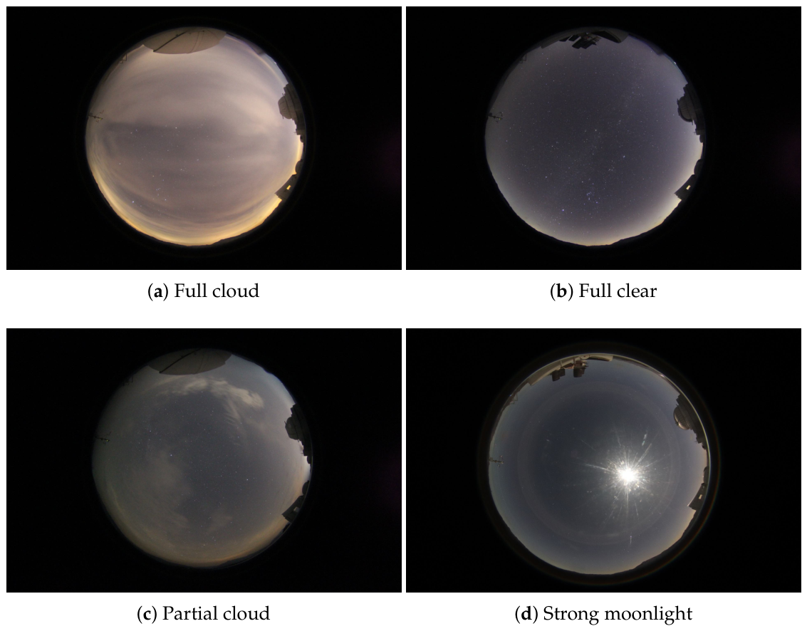
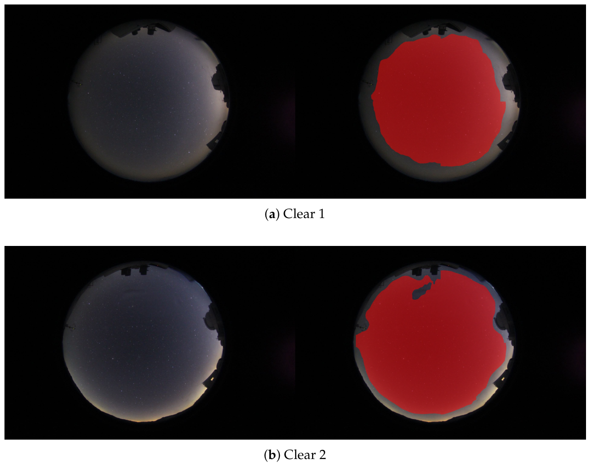
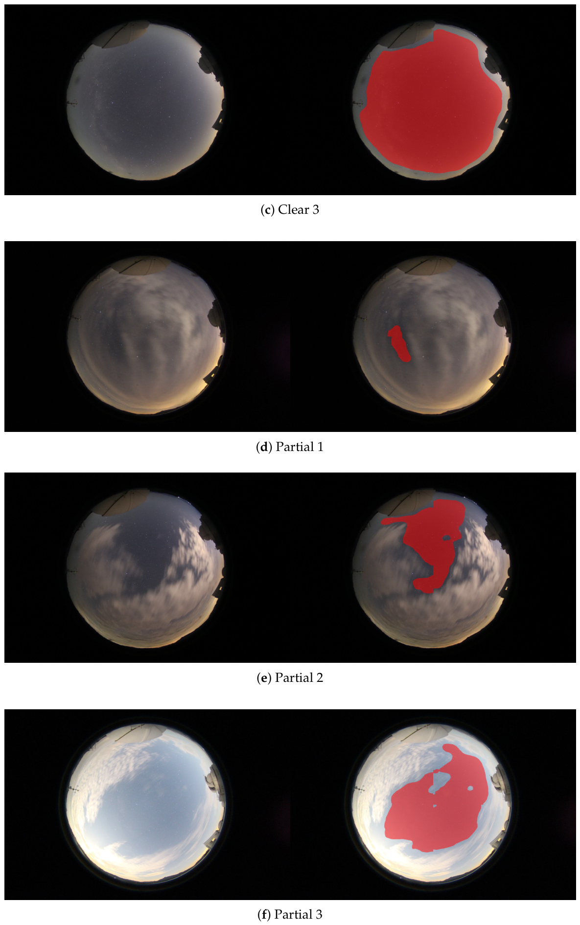
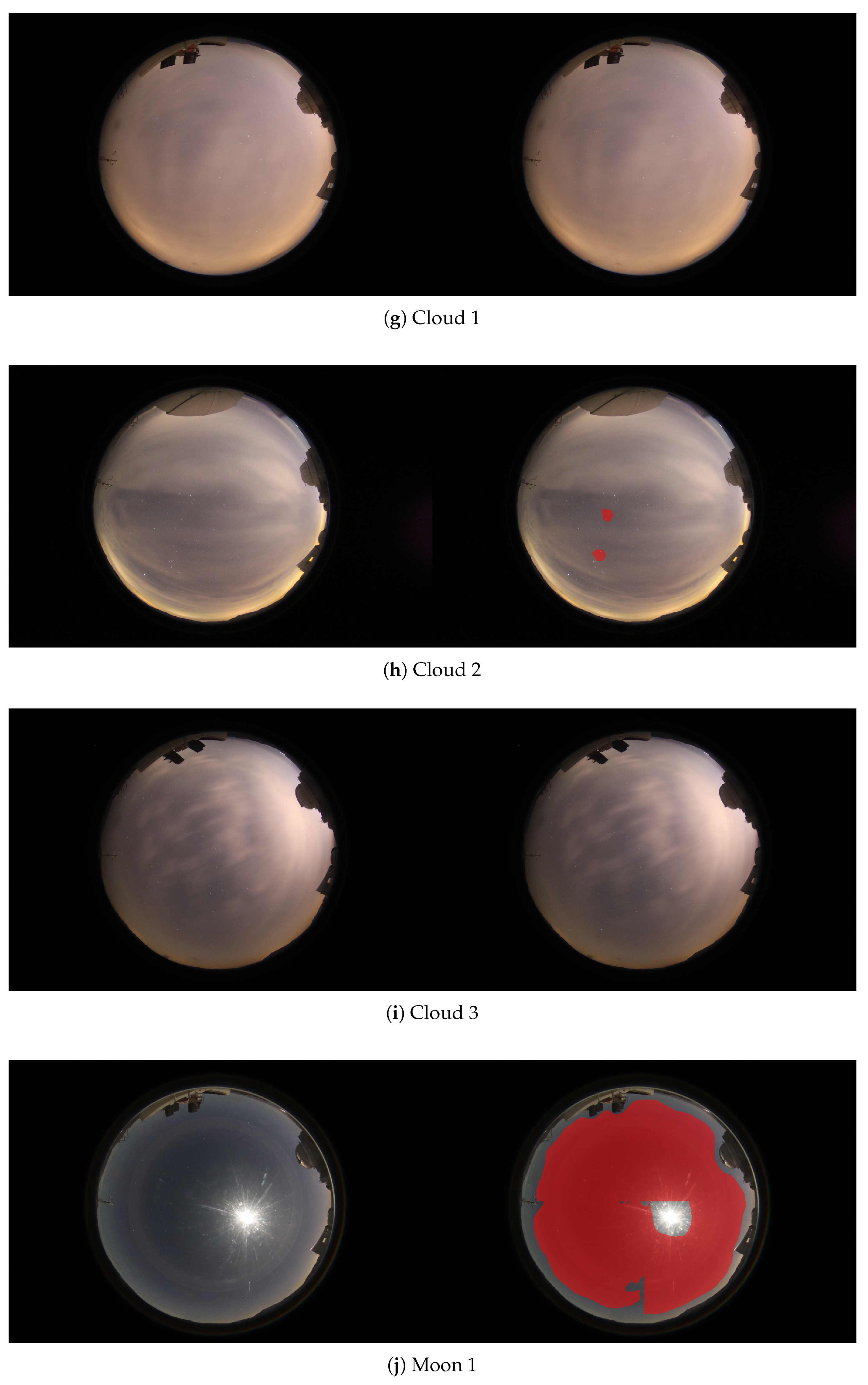
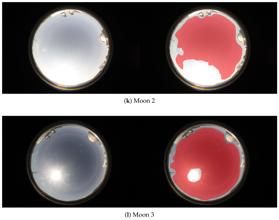
The raw dataset comprises continuous all-sky fisheye images acquired at Xinglong Observatory between 2022 and 2025. The all-sky camera uses a Canon C600 CCD (Canon Inc., Tokyo, Japan) with a focal length of 4.5 mm. The dataset contains approximately 90,000 fisheye images with a sampling interval of about 5.5 min, occupying roughly 60 GB of storage. It covers various weather and illumination conditions, including fully clear, fully cloudy, partially cloudy, and strong moonlight scenes, as illustrated in Figure 1.

Regarding weather distribution, the dataset contains a comparable number of clear-sky images and images taken under other weather conditions. Strong moonlight scenes result from the relatively high exposure settings used during all-sky camera operation.

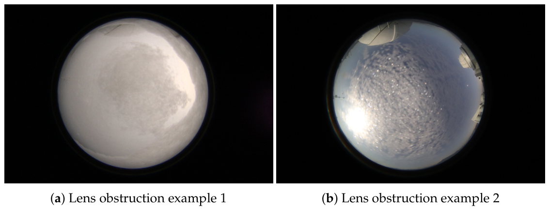
Furthermore, adverse conditions such as rain, snow, or ice accumulation on the lens can occasionally obstruct all-sky camera observations, as shown in Figure 2.

2.2. Data Preprocessing

To ensure the uniformity of the data, we first perform a series of data preprocessing procedures as follows:

• Resolution Unification. The original dataset contains images with multiple resolutions, including $1920\times 1280$, $2976\times 1984$, and $5184\times 3456$, among which $1920\times 1280$ accounts for the largest proportion. We developed scripts to adjust the resolutions and unified all images to $1920\times 1280$. This reduces the storage and training overhead while preserving essential information.
• EXIF Orientation Tag Unification. The original images are stored as JPEG files, while their metadata are recorded using the EXIF standard embedded in the JPEG file structure. Among these metadata, the orientation tag specifies the rotation and flipping state of the image. Different values from 1 to 8 correspond to different rotation or mirroring operations, indicating that the image may have been rotated or flipped during acquisition or storage. To avoid alignment errors caused by such transformations, we normalized all images by setting their orientation tags to 1 (no rotation).
• Time Unification. The original dataset includes all-day fisheye images. However, since our observations focus mainly on nighttime, we retained only data from 17:00 to 06:00 the next morning.

2.3. Training and Test Data Generation

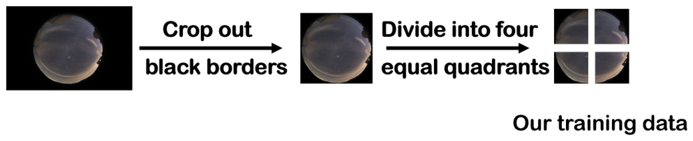
We first select over 300 fisheye images from the preprocessed raw data, covering four weather conditions (clear sky, overcast, moonlit, and partly cloudy) with an approximate ratio of 1:1:1:3. Using Labelme as the standard tool for semantic segmentation, we annotate the sky regions observable at the time of each capture. For data augmentation, we then crop and split each annotated full image into four parts (Figure 3), resulting in a training dataset of over 1200 cropped fisheye images.

Additionally, we construct a test set to evaluate our model, comprising a total of 129 fisheye images at their original size that cover a variety of sky conditions.

2.4. Astrometry

We adopt the astrometric method of [18] for super-wide field-of-view images. The transformation from pixel coordinates $(x,y)$ to horizon coordinates (azimuth A and zenith distance Z) is given by:

$$\begin{array}{cc}\hfill c_a& =atan2(x-x_0,y-y_0)+\pi ,r=\sqrt{{(x-x_0)}^2+{(y-y_0)}^2},\hfill \end{array}$$

(1)

$$\begin{array}{cc}\hfill u& =k_{1}r+k_2{r}^3+k_3{r}^5+k_4{r}^7,\hfill \end{array}$$

(2)

$$\begin{array}{cc}\hfill Z& =arccos\left(cosucose-cos((a_0-E)+c_a)sinusine\right),\hfill \end{array}$$

(3)

$$\begin{array}{cc}\hfill A& =E+atan2\left(sin((a_0-E)+c_a)sinu,cos((a_0-E)+c_a)sinucose+cosusine\right),\hfill \end{array}$$

(4)

where $(x_0,y_0)$ is the projection centre; $E,a_0,e$ are the camera orientation parameters relative to the zenith; and the Kannala–Brandt equation $u=T\left(r\right)$, where u denotes the distorted angular distance from the optical axis, models the radial distortion of the fisheye lens [22].

For observation replanning, the inverse transform from a target horizon direction back to image coordinates is equally important. Let $z=\pi /2-\mathrm{Alt}$ denote the zenith distance corresponding to a target altitude $\mathrm{Alt}$, and let $a=A$ be its azimuth. The angular separation $u_0$ between the target direction and the optical axis is obtained from the inverse spherical relation

$$\begin{array}{cc}\hfill u_0& =arccos\left(coszcose+sinzsinecos(a-E)\right).\hfill \end{array}$$

(5)

Defining the intermediate angle $b=(a_0-E)+c_a$, the image-plane azimuth is recovered by

$$\begin{array}{cc}\hfill b& =atan2\left({\displaystyle \frac{sin(a-E)sinz}{sin{u}_0}},-{\displaystyle \frac{cosz-cos{u}_{0}cose}{sin{u}_{0}sine}}\right),\hfill \end{array}$$

(6)

$$\begin{array}{cc}\hfill c_a& =b-a_0+E(mod2\pi ).\hfill \end{array}$$

(7)

The required image radius r is then obtained by numerically solving the monotonic Kannala–Brandt equation

$$\begin{array}{c}\hfill u_0=k_{1}r+k_2{r}^3+k_3{r}^5+k_4{r}^7,\end{array}$$

(8)

after which the pixel coordinates follow from

$$\begin{array}{cc}\hfill x& =x_0+rsin(c_a-\pi ),\hfill \end{array}$$

(9)

$$\begin{array}{cc}\hfill y& =y_0+rcos(c_a-\pi ).\hfill \end{array}$$

(10)

In other words, the inverse mapping consists of an analytic inversion of the spherical orientation relations followed by a numerical inversion of the fisheye radial distortion model. This formulation is exactly the one used in our implementation for projecting scheduled targets onto the real-time segmentation mask.

The calibration consists of two core steps. First, using 20 reference stars obtained from a photometry process, with known equatorial coordinates, we iteratively fit the distortion coefficients $k_{1\dots 4}$ and the orientation parameters $(E,a_0,e)$ by least squares. Second, the optical centre $(x_0,y_0)$ is refined by analyzing the sinusoidal pattern in the azimuth residuals: the amplitude of this pattern is minimized over a grid around the initial centre, yielding pixel-level accuracy. Once calibrated, the forward mapping from pixel coordinates to $(A,\mathrm{Alt})$, where $\mathrm{Alt}=\pi /2-Z$, is obtained by direct evaluation of the forward model, whereas the inverse mapping uses the analytic–numeric procedure above. Since all calibration parameters are stored after fitting, subsequent images can be mapped without repeating the calibration step, making both the forward and inverse transforms fast enough for real-time replanning.

3. Method

Semantic segmentation of all-sky images is performed using DeepLab-v3 [15], a convolutional neural network that classifies each pixel into “observable” or “unobservable” categories based on cloud. To enable real-time execution on the embedded hardware of the observation system, we adopt MobileNetV3 [23] as the lightweight backbone, which significantly reduces inference latency with minimal accuracy loss. Training data are prepared using Labelme [24], a manual annotation tool with which an operator labels polygon-shaped regions of sky availability on a set of representative all-sky images. The trained model outputs a binary segmentation mask for each incoming image, providing a semantic weather constraint that feeds directly into the dynamic observation replanning logic.

3.1. Observable Region Recognition

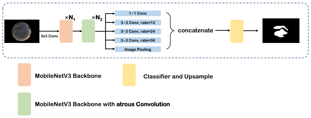
We adopt DeepLabV3 with a MobileNetV3 backbone from the torchvision library1 to predict observable regions in all-sky fisheye images. Figure 4 illustrates the overall model architecture.

The input image first passes through a $3\times 3$ convolution, followed by multiple MobileNetV3 bottleneck layers, where we set $N_1=12$ and $N_2=3$. The resulting feature maps are then fed into the ASPP module, which consists of five parallel branches: a $1\times 1$ convolution; three $3\times 3$ atrous convolutions with dilation rates of 12, 24, and 36; and a global pooling branch (AdaptiveAvgPool2d(1) followed by a $1\times 1$ convolution). The outputs of all branches are concatenated, reduced in dimension, fed into the classification head, and finally upsampled to produce the segmentation mask.

We chose the MobileNetV3 backbone for its lightweight design and fast inference speed. The total number of parameters in the model is approximately 11.02 million. We trained the model from scratch using our prepared training data. During training, we set the batch size to 32, the number of epochs to 400, and the learning rate to 0.01.

3.2. Observation Sequence Replanning

The final step is to validate the observation sequence using the all-sky camera mask. With the pixel-to-horizontal coordinate mapping established and the observable region identified, we can check whether a scheduled target is actually observable before slewing to it, by using a all-sky camera image, an R.A., Dec. coordinate and the observation time through a Python 3.9.21 function. If not, a replanning process is triggered.

Two replanning strategies are implemented: one for general-purpose telescopes and another for survey telescopes. For general telescopes, the algorithm examines the remaining unobserved targets in the original sequence. It searches for the first target that satisfies the following observability criteria within the upcoming observation time window: (1) altitude consistently above $30°$, and (2) angular separation from the Moon at least $15°$. Once such a target is found, it is moved forward to the current time, while the displaced targets are recorded for later execution. The search continues until a suitable target is identified or the list is exhausted. If no targets are available, the upcoming observation time window remains the same, and nothing will be done.

For survey telescopes, such as those used in the Nearby Galaxy Supernova Survey [20], the observation strategy is fixed and relies on an input catalog. The input catalog contains the coordinates and distances of galaxies within 50 Mpc. To serve the purpose of the survey, bright galaxies are retained while fainter ones are excluded. This selection is performed by filtering based on galaxy ID prefixes—for example, galaxies with designations such as NGC, ESO, IC, and UGC are preserved. An additional trimming criterion is observability from Xinglong Observatory. After these filtering steps, the input catalog yields 3772 galaxies. The same altitude and Moon-separation constraints apply, with an additional preference for targets currently crossing the meridian. Rescheduling is triggered at every target switch, and the input catalog is scanned to select the best-observable object. In both strategies, the output is a revised observation sequence. We generate the output in the ninaTargetSet format, which is the sequencer control file for Nighttime Imaging ‘N’ Astronomy (N.I.N.A.)2, a widely used observation control system among astronomical amateurs. The ninaTargetSet file contains fields such as filter control and focus control; however, in this process, only the target’s right ascension, declination, and name are modified.

4. Result

4.1. Semantic Segmentation Model Evaluation

We have now completed training and evaluated the model on the test set, and the quantitative results are presented in

Table 1. Segmentation performance under different weather conditions. Overcast images contain no observable regions in their ground-truth masks; therefore, standard segmentation metrics (IoU, Accuracy, Precision, Recall, F1) are not applicable. We instead use FPR-based evaluation. ↑ indicates higher is better, and ↓ indicates lower is better.

Condition	IoU ↑	Acc ↑	Prec ↑	Rec ↑	F1 ↑	FPR ↓	Max FPR ↓	Avg FPR ↓
Partly Cloudy	0.67	0.97	0.80	0.81	0.80	—	—	—
Clear Sky	0.87	0.96	0.99	0.88	0.93	—	—	—
With Moon	0.89	0.97	0.97	0.92	0.94	—	—	—
Overcast	—	—	—	—	—	0.01	0.08	0.01

.

The meanings of these evaluation metrics are as follows. In brief, IoU measures the overlap between the predicted and ground-truth observable regions, Accuracy reflects the overall pixel-wise correctness, Precision and Recall quantify the reliability and completeness of observable-region detection, and the F1-score summarizes the balance between Precision and Recall. Let $y\left(x\right)\in \{0,1\}$ denote the ground-truth label of pixel x, and $\widehat{y}\left(x\right)\in \{0,1\}$ denote the predicted label, where 1 represents foreground and 0 represents background. The four basic statistics in the confusion matrix are defined as $TP=\left|\right\{x\mid y\left(x\right)=1,\widehat{y}\left(x\right)=1\left\}\right|$, $FP=\left|\right\{x\mid y\left(x\right)=0,\widehat{y}\left(x\right)=1\left\}\right|$, $FN=\left|\right\{x\mid y\left(x\right)=1,\widehat{y}\left(x\right)=0\left\}\right|$, and $TN=\left|\right\{x\mid y\left(x\right)=0,\widehat{y}\left(x\right)=0\left\}\right|$, where $|·|$ denotes the number of pixels in the corresponding set.

Based on the above definitions, each evaluation metric is computed as $\mathrm{IoU}={\displaystyle \frac{TP}{TP+FP+FN}}$, $\mathrm{Accuracy}={\displaystyle \frac{TP+TN}{TP+TN+FP+FN}}$, $\mathrm{Precision}={\displaystyle \frac{TP}{TP+FP}}$, $\mathrm{Recall}={\displaystyle \frac{TP}{TP+FN}}$ and $\mathrm{F}1\text{-}\mathrm{Score}={\displaystyle \frac{2·\mathrm{Precision}·\mathrm{Recall}}{\mathrm{Precision}+\mathrm{Recall}}}$.

Furthermore, to measure the tendency of the model to misclassify background pixels as foreground, we introduce the False Positive Rate (FPR), defined as

$$\mathrm{FPR}={\displaystyle \frac{FP}{FP+TN}}.$$

(11)

For a dataset containing N test images, let ${\mathrm{FPR}}_i$ denote the false positive rate of the i-th image. The average and maximum false positive rates are respectively defined as

$${\mathrm{FPR}}_{\mathrm{avg}}={\displaystyle \frac{1}{N}}{\displaystyle \sum _{i=1}^N}{\mathrm{FPR}}_i,$$

(12)

$${\mathrm{FPR}}_{max}=\underset{1\le i\le N}{max}{\mathrm{FPR}}_i.$$

(13)

The segmentation results on part of the test set are shown in Figure 5.

4.2. Observation Efficiency

In this section, we present a quantitative evaluation of our replanning method. The test sequences are taken from real observing sequences of the Nearby Galaxy Supernova Survey, focusing on periods when clouds partially covered the sky—conditions that typically render many originally scheduled targets unobservable. For each time step, we compare our replanned sequences against the original ones using two observability criteria, both with and without the all-sky camera mask, to determine which targets are actually observable.

Table 2. Representative observation replanning results selected from the 49 tested sequences. UTC gives the start time of the evaluated interval. “Orig.” denotes the original NGSS schedule, whereas “Our” denotes the schedule after replanning. “Obs.” and “Unobs.” are the numbers of observable and unobservable targets, respectively, “ObsRate” is the observable fraction within the interval, and “Replanning Count” is the number of target substitutions performed by our scheduler.

UTC	Duration (h)	Orig. Obs.	Orig. Unobs.	Orig. ObsRate	Our Obs.	Our Unobs.	Our ObsRate	Replanning Count
22 January 2024 T16:02:08	2.5636	6	16	27.3%	21	1	95.5%	15
17 January 2024 T12:52:10	2.3150	0	20	0.0%	4	16	20.0%	4
29 March 2024 T12:42:26	2.1567	0	18	0.0%	1	17	5.6%	1
7 April 2024 T17:52:11	2.9503	4	17	19.0%	6	15	28.6%	2
31 May 2024 T13:08:42	1.9481	0	14	0.0%	2	12	14.3%	2
17 June 2024 T16:00:58	2.9686	17	5	77.3%	22	0	100.0%	5
24 September 2024 T16:54:37	2.5686	0	22	0.0%	22	0	100.0%	22
4 October 2024 T12:17:14	2.8819	20	5	80.0%	25	0	100.0%	5
14 February 2025 T12:02:44	3.8903	0	33	0.0%	32	1	97.0%	32
24 February 2025 T16:00:32	4.7489	3	38	7.3%	39	2	95.1%	36

presents 10 representative cases selected from the 49 test sequences summarized in our batch evaluation. Across all 49 tests, the mean observability rate of the original plans is only 19.0%, whereas the replanned sequences reach 79.1%, corresponding to an average gain of 60.1 percentage points. The selected examples intentionally cover different situations: cases with dramatic improvement (e.g., 24 September 2024 and 14 February 2025), cases where the original schedule is already reasonably good but replanning still further improves it (e.g., 17 June 2024 and 4 October 2024), and cases with only limited but still positive gains under unfavorable sky conditions (e.g., 17 February 2024, 29 March 2024, and 31 May 2024). The rightmost column lists the replanning count, i.e., the number of target substitutions performed during the corresponding interval. These results demonstrate that integrating the all-sky camera’s pixel-to-horizontal mapping with a conservative but reliable cloud mask enables robust real-time rescheduling, substantially enhancing effective observing efficiency under non-ideal weather conditions.

Furthermore, the total time required to perform all sequence adjustments and statistical tasks on 100 consecutive fisheye images is 499.39 s using an AMD Ryzen 7 4800U with Radeon Graphics (1.80 GHz) processor(Advanced Micro Devices, Santa Clara, CA, USA), which is about 5 s per image and considered acceptable.

5. Discussion

5.1. Horizon Calibration Accuracy

To evaluate the precision of our all-sky camera astrometric calibration, we selected the brightest celestial objects from a single clear night and compared their computed horizon coordinates with the true values derived from precise ephemerides.

Table 3. Astrometric errors for the brightest stars in one all-sky camera image.

Name	Time (UTC)	Alt Error (deg)	Az Error (deg)
Jupiter	18 February 2025 19:53:23	0.09	0.20
Capella	18 February 2025 19:53:23	0.10	0.65
Mirfak	18 February 2025 19:53:23	0.22	0.08
Menkalinan	18 February 2025 19:53:23	0.03	0.67
Mars	18 February 2025 19:53:23	0.02	0.08
Theta Aurigae	18 February 2025 19:53:23	0.02	0.04
Aldebaran	18 February 2025 19:53:23	0.10	0.15

summarizes the azimuth and altitude errors for each object. As shown, the absolute errors are consistently below $1°$, with most well below $0.5°$. Given that the plate scale of our camera is approximately $0.17°$ per pixel, a typical azimuth or altitude error corresponds to only a few pixels. In fact, the root-mean-square error is on the order of $0.2$–$0.3°$, which is roughly equivalent to $1.2$–$1.8$ pixels. Therefore, the astrometric uncertainty introduced by our calibration is negligible for the purpose of observation replanning and sky-availability masking. It does not meaningfully affect the projection of celestial targets onto the image plane nor the inverse mapping from pixel coordinates to horizon directions. Consequently, the subsequent decision-making process—such as checking whether a target falls inside the observable mask—remains robust and accurate.

5.2. Current Shortcomings

Our work has two main limitations. First, our observability criteria are relatively strict compared to real observing conditions. For instance, thin cirrus clouds or light haze may still allow useful scientific exposures; however, during our annotation process, we labeled only the most reliably observable sky regions. This conservative choice was driven by two considerations: (1) the need to obtain high-quality photometric data from observations, as partially cloudy conditions would complicate subsequent photometric processing, and (2) the requirement that any region labeled as “observable” must indeed be usable without risk. As a result, some partially cloudy or slightly obscured areas are excluded, potentially leading to an underestimation of the truly accessible sky.

Second, we have not explicitly optimized for weather disturbances such as dew, frost, snow, or dust on the camera window. Many robotic telescopes already suspend observations under such conditions, and we therefore did not implement dedicated handling for them. Nevertheless, the all-sky camera itself can serve as a valuable sensor for recognizing these adverse weather events. By integrating real-time image analysis (e.g., detecting frost patterns or dust spots), future work could not only improve the robustness of rescheduling but also provide input for short-term weather forecasting at the observatory site.

5.3. Future Plan

In the nearer term, we plan to improve the current pipeline in several directions. First, we will continue to collect and annotate all-sky images covering thin cirrus clouds, haze, and various adverse weather conditions, such as snow, fog, and blowing dust, to retrain and refine the semantic segmentation model, thereby expanding its capability beyond the current conservative “clear or not” binary classification. Second, we will generalize the scheduling logic to support field-based observing modes: instead of checking only the single target coordinate at the central of view, the scheduler will accept the four corner coordinates of a requested sky region and verify that the entire field is observable. This enhancement is motivated by the future wide-field survey needs of projects like GOTTA, and we plan to develop the corresponding pipeline after investigating the specific requirements. Third, we aim to incorporate cloud motion prediction into the decision loop. Currently, the system does not predict cloud movement or elongate masks along wind direction, primarily because the readily available regional wind data for North China do not accurately represent the local conditions at the Xinglong mountain site. We therefore plan to develop methods for estimating local wind and cloud motion vectors directly from sequential all-sky camera frames, which will enable more reliable short-term cloud forecasting and wind-aware scheduling.

Future work will also further explore extending the current all-sky camera replanning pipeline into a Vision–Language–Action (VLA) framework for real-time all-sky observation replanning to serve as an important skill of the AI Astronomer. VLA models offer a new direction for minimizing manual rule-based interfaces. These models typically take visual observations and task instructions as input and directly generate actions or decisions to interact with the environment, demonstrating strong cross-task generalization and few-shot adaptation capabilities in robotic control [25,26]. In the context of astronomical observation, the action space can be defined as scheduling actions such as target reordering, observation delays, switching to candidate targets, adjusting exposure strategies, or triggering safe shutdowns. Meanwhile, language inputs can encode scientific priorities, observational constraints, weather risks, and human policy preferences.

Subsequently, we can first construct a demonstration dataset of “all-sky images, masks, candidate targets, and replanning actions” using historical logs generated by the current pipeline, treating the existing rule-based system as a teacher policy. Furthermore, by drawing on approaches for multi-task data, action representation, and parameter-efficient fine-tuning from works such as Open X-Embodiment and OpenVLA, we can establish a unified action representation tailored for observation scheduling tasks. By fine-tuning open-ended VLA models or training lightweight policy heads, we aim to achieve a direct mapping from images and task contexts to scheduling actions [26,27,28].

6. Conclusions

We have presented a complete pipeline for cloud-adaptive observation replanning based on all-sky camera images. The key components include: (i) a curated dataset of fisheye images under diverse sky conditions; (ii) a DeepLabV3-MobileNetV3 model that achieves high segmentation accuracy for observable sky regions; (iii) an astrometric calibration that establishes a precise pixel-to-horizon mapping with sub-degree errors; and (iv) a rule-based replanning module that dynamically substitutes blocked targets while respecting altitude and lunar-separation constraints. Extensive tests on real survey data show that our method raises the observability rate from typically below 10% to over 90% during partially cloudy periods, substantially improving observing efficiency without requiring additional hardware.