Dynamics of a Classical Bi-Metric Cosmology with GUP-Deformed Poisson Brackets

Abstract

This work analyzes a bi-metric cosmological model where two sectors, characterized by their respective scale factors, interact through a deformed Poisson bracket structure. This deformation is based on the Generalized Uncertainty Principle (GUP). Through a numerical analysis, we study how this interaction affects the expansion dynamics. The results indicate that for positive values of the deformation parameter, the coupling induces an acceleration that leads to a Big Rip singularity in finite time, even in the absence of a cosmological constant. A power-law relation is established between the deformation parameter and the critical time of divergence for the scale factors. Finally, the regime with a negative deformation parameter is also investigated. In this case, the symplectic structure becomes singular, leading to the contraction of one sector and the freezing of the other.

1. Introduction

Despite the great success of the cosmological standard model, $\Lambda$CDM [1], several fundamental issues remain unresolved. In particular, the origin and nature of dark energy (DE) and dark matter (DM) [2,3,4,5,6,7,8], as well as the persistence of the initial cosmological singularity [9,10,11], are aspects where $\Lambda$CDM provides phenomenological fits but lacks a fully satisfactory theoretical explanation.

Exploring new routes to address these problems may help to better understand them. Several approaches have been proposed in the literature, including the incorporation of scalar fields in cosmological models such as quintessence, K-essence, tachyon fields or phantom models [12,13,14,15,16]. Other alternatives include causal-set inspired models [17,18], Chaplygin gas [19], running $\Lambda$ scenarios [20], or modifications to GR [21]. These proposals illustrate the wide effort devoted to extending the standard cosmological paradigm.

An independent route to addressing the aforementioned discrepancies incorporates phenomenological signatures expected from quantum gravity (QG). One of the most widely discussed features, which is pertinent to the present work, is the appearance of a minimal observable length. Early indications of such a fundamental scale in gravity can be traced back to the pioneering work of Bronstein [22], who analyzed the quantization of weak gravitational fields.

At a phenomenological level, the presence of a minimal length is often implemented through modifications of the Heisenberg uncertainty principle. The resulting framework is known as the Generalized Uncertainty Principle (GUP), which encompasses a variety of proposals motivated by different theoretical considerations [23,24]. These motivations include quantum geometry [25], gedankenexperiments involving gravitational effects [26,27], black-hole (BH) physics [26,28], polymer quantization [29], and heuristic arguments based on quantum gravitational considerations [30].

The implications of the GUP in gravitational systems have been intensively explored in the literature (see [31] and references therein). For instance, several modifications to the Schwarzschild metric have been derived in [32,33,34] in order for the resulting geometry to be consistent with the GUP-corrected Hawking temperature. The absence of the $r=0$ singularity in Schwarzschild black holes has been shown within specific frameworks [35] using the Ashtekar–Barbero connection formalism, and more generally in other approaches to regular black holes [36]. The existence of BH remnants has been studied in [37,38,39]; an important consequence consists in preventing the complete evaporation of the BH [40,41] thereby avoiding the divergence in the emitted radiation when $M_{BH}\to 0$. Other works have analyzed the impact of the GUP on BH thermodynamics [37,39,42,43,44], BH shadows and scattering processes [45,46], as well as modifications of quantum field theory in curved backgrounds [40,41,47]. Another consequence is the appearance of logarithmic corrections to the entropy-area relation of black holes [43].

Cosmological applications of the GUP framework have also been widely investigated. Minimal-length corrections have been implemented in Friedmann–Lemaître–Robertson–Walker cosmologies [48], Bianchi models [49,50], Szekeres space-times [51], and Einstein static universes [52,53]. In many of these studies, the presence of a minimal length leads to interesting phenomena such as the removal of the initial cosmological singularity and the appearance of bouncing solutions [48,54].

The phenomenological implications of the GUP framework have also been constrained using observational data. For instance, upper bounds on the deformation parameter have been obtained from the gravitational-wave event GW150914 [55]. Additionally, constraints on a rescaled deformation parameter were derived from the analysis of twisted light in the vicinity of the supermassive BH M87* [56]. Astrophysical systems at much lower energy scales can also provide relevant bounds: for example, the modification of the Jeans mass induced by GUP corrections has been used to constrain the deformation parameter by requiring consistency with the observed mass and temperature of Bok globules [57].

From a phenomenological perspective, several approaches have been proposed to place bounds on the parameters of the Generalized Uncertainty Principle using low-energy and precision measurement systems. These proposals include, for instance, neutron interferometry [58], cold-atom systems [59], phonon cavities [60], and optomechanical setups through the analysis of quantum noise [61]. These works aim at testing possible quantum-gravity-induced modifications of quantum mechanics in experimentally accessible regimes.

From the gravitational side only, another interesting framework to explore cosmological dynamics consists in considering models with more than one scale factor. In particular, bi-metric cosmological models describe the universe in terms of two metric sectors, each characterized by its own scale factor.

In the formulation proposed in [62,63,64], the interaction between these sectors is induced through a deformation of the Poisson bracket structure of the minisuperspace variables. This deformation, motivated by ideas inspired by quantum gravity, generates an effective coupling between the two cosmological patches.

This class of models exhibits several interesting features. In particular, the model proposed in [62] can account for the accelerated expansion of the universe through the interaction between the two cosmological patches, induced by the deformation of the symplectic structure, without the need to introduce an explicit dark energy component. When matter sources are included [65,66], the model becomes an example of a non-standard cosmology with a rich dynamical structure.

In this work we investigate the interplay between bi-metric cosmology and a minimal-length structure inspired by the Kempf algebra. We consider two FLRW scale factors associated with two metric sectors and implement minimal-length effects at the classical level through a GUP-inspired deformation of the Poisson bracket algebra of the minisuperspace variables. Our aim is to determine how these minimal-length corrections modify the coupled dynamics of the scale factors and whether they can generate new cosmological behaviors within this framework.

Our main results can be summarized as follows. First, the classical GUP deformation naturally induces communication between the two cosmological patches, in a way reminiscent of non-commutative models. Second, the deformation becomes dynamically relevant at late times, leading to a super-accelerated evolution that culminates in a Big-Rip-type behavior. Third, we find that the critical time at which the scale factors and Hubble parameters diverge follows a power-law relation with the deformation parameter. Finally, we extend the analysis to negative values of the deformation parameter, showing that the symplectic structure becomes degenerate: in this regime one patch effectively freezes while the other undergoes a total contraction.

The remainder of the paper is organized as follows. In Section 2 we review the main aspects of the bi-metric cosmological model and introduce the GUP-inspired deformation of the canonical algebra. In Section 3 we analyze the dynamical evolution of the system through numerical solutions. Section 4 is devoted to studying the relation between the deformation parameter and the rip time. In Section 5 we discuss the behavior of the system for negative values of the deformation parameter. Finally, Section 6 contains our conclusions and discussion.

2. Formalism: Deformed Algebra and Hamiltonian

The most studied form of the GUP corresponds to the quadratic GUP [26,67] (see also [68] for a systematic treatment of the quantum mechanics associated with this GUP) where the uncertainty in position ($\Delta x$) and momentum ($\Delta p$) in one dimension satisfies (for the N-dimensional case see, for example, [50,69])

$$\Delta x\Delta p\ge {\displaystyle \frac{ħ}{2}}(1+\beta \Delta p^2),$$

(1)

where $\beta$ is the deformation parameter. The $\Delta p^2$ modification implies a minimal position uncertainty $\Delta x_{min}=ħ\sqrt{\beta }$, thereby introducing a minimal-length scale in the theory.

A possible way to obtain this quadratic GUP is through a deformation of the canonical algebra between x and p:

$$[x,p]=iħ(1+\beta p^2).$$

In this work we use the algebra proposed by Kempf, Mangano and Mann [68] due to its simplicity, its direct minimal-length implication, and because it obeys the Jacobi identities to all orders in the deformation parameter $\beta$. The algebra reads

$$\begin{array}{c}\hfill [x_i,p_j]=iħ{\delta }_{ij}(1+\beta p^2),\\ \hfill [x_i,x_j]=2iħ\beta (p_i{x}_j+p_j{x}_i),\end{array}$$

(2)

with $p^2={\sum }_i{p}_i^2$. This algebra is obtained by assuming a minimal modification to the one-dimensional commutator of x and p of the form $(1+\beta p^2)$ and by imposing that the momenta commute, $[p_i,p_j]=0$. The GUP modification in Equation (2) does not break the translational and rotational symmetries of the underlying theory [68].

We implement Equation (2) at the classical level to mimic the GUP algebra associated with a minimal-length structure in the underlying quantum theory. Within this approach, the deformed commutation relations are translated into modified Poisson brackets that preserve the standard properties of the Poisson algebra, namely antisymmetry, linearity, the Leibniz rule, and the Jacobi identity (see [70,71,72,73,74] for a detailed discussion on the classical limit of the GUP).

In the cosmological minisuperspace model considered here, the canonical variables are the scale factors a and b together with their conjugate momenta ${\pi }_a$ and ${\pi }_b$. Motivated by the GUP-induced deformation of the phase-space structure, we assume that these variables satisfy a modified Poisson algebra obtained as the classical limit of the corresponding deformed commutators

$$\begin{array}{cc}\hfill \{a,b\}& =2\beta ({\pi }_{a}b-{\pi }_{b}a),\hfill \\ \hfill \{a,{\pi }_a\}=1& +\beta {\mathit{\pi }}^2=\{b,{\pi }_b\},\hfill \end{array}$$

(3)

with ${\mathit{\pi }}^2={\pi }_a^2+{\pi }_b^2$. A key feature of this deformed phase-space structure is that the scale factors a and b acquire a nonvanishing Poisson bracket, $\{a,b\}\ne 0$ and, as a result, the evolution of the two cosmological sectors becomes dynamically coupled, with the strength of the interaction controlled by the GUP parameter $\beta$.

In the bi-metric model considered here, two scale factors describe the evolution of the universe. These might represent two causally disconnected patches [75] of the same universe or even two different universes in a sort of multiverse scenario [76].

The Hamiltonian of this model comes from two non-interacting copies of the Hilbert-Einstein action [62]

$$\mathcal{H}=N\left[{\displaystyle \frac{G_{\mathrm{N}}}{2}}\left({\displaystyle \frac{{\pi }_a^2}{a}}+{\displaystyle \frac{{\pi }_b^2}{b}}\right)-{\displaystyle \frac{{\Lambda }_a}{6{\mathrm{G}}_N}}{a}^3-{\displaystyle \frac{{\Lambda }_b}{6{\mathrm{G}}_N}}{b}^3\right],$$

(4)

where N is the lapse function, a and b are the scale factors, and ${\pi }_a$ and ${\pi }_b$ are their canonical conjugate momenta, respectively. The cosmological constants are, on each patch, ${\Lambda }_a$ and ${\Lambda }_b$, while $G_N$ is Newton’s constant. We have also set the three-dimensional curvature $k_a=k_b=0$, to be consistent with present bounds [77].

This type of model has been discussed in different scenarios. For example, inflation has been discussed in [62]. A Poisson bracket deformation including a non-trivial bracket between scale factors was discussed in [63,64]. In [65], the presence of matter in the model was considered.

Using the Hamiltonian (4) together with the deformed Poisson brackets (3), the equations of motion follow from Hamilton’s equations.

$$\begin{array}{cc}\hfill \dot{a}& =G_{\mathrm{N}}{\displaystyle \frac{{\pi }_a}{a}}(1+\beta {\mathit{\pi }}^2)-\beta \left(G_{\mathrm{N}}{\left({\displaystyle \frac{{\pi }_b}{b}}\right)}^2+{\displaystyle \frac{{\Lambda }_b}{G_{\mathrm{N}}}}{b}^2\right)\left({\pi }_{a}b-{\pi }_{b}a\right),\hfill \end{array}$$

(5)

$$\begin{array}{cc}\hfill \dot{b}& =G_{\mathrm{N}}{\displaystyle \frac{{\pi }_b}{b}}(1+\beta {\mathit{\pi }}^2)+\beta \left(G_{\mathrm{N}}{\left({\displaystyle \frac{{\pi }_a}{a}}\right)}^2+{\displaystyle \frac{{\Lambda }_a}{G_{\mathrm{N}}}}{a}^2\right)\left({\pi }_{a}b-{\pi }_{b}a\right),\hfill \end{array}$$

(6)

$$\begin{array}{cc}\hfill {\dot{\pi }}_a& ={\displaystyle \frac{1}{2}}\left(G_{\mathrm{N}}{\left({\displaystyle \frac{{\pi }_a}{a}}\right)}^2+{\displaystyle \frac{{\Lambda }_a}{G_{\mathrm{N}}}}{a}^2\right)(1+\beta {\mathit{\pi }}^2),\hfill \end{array}$$

(7)

$$\begin{array}{cc}\hfill {\dot{\pi }}_b& ={\displaystyle \frac{1}{2}}\left(G_{\mathrm{N}}{\left({\displaystyle \frac{{\pi }_b}{b}}\right)}^2+{\displaystyle \frac{{\Lambda }_b}{G_{\mathrm{N}}}}{b}^2\right)(1+\beta {\mathit{\pi }}^2).\hfill \end{array}$$

(8)

Here, the gauge $N=1$ is used. The constraint ${\dot{\pi }}_N=0$, the canonical conjugate of N, gives rise to the equation

$${\displaystyle \frac{{\pi }_a^2}{a}}+{\displaystyle \frac{{\pi }_b^2}{b}}={\displaystyle \frac{{\Lambda }_a}{3G_{\mathrm{N}}^2}}{a}^3+{\displaystyle \frac{{\Lambda }_b}{3G_{\mathrm{N}}^2}}{b}^3.$$

(9)

For numerical purposes, it is convenient to write the previous set of equations in terms of dimensionless quantities. To do that, it is enough to redefine fields according to

$$\tilde{a}=\mu a{\tilde{\pi }}_a=\mu G_{\mathrm{N}}{\pi }_a,$$

(10)

with $\mu$ an inverse-length (time) scale (or energy, in natural units). Similar re-scalings are performed on the sector b variables. We also define the dimensionless variables

$$\beta \equiv \kappa G_{\mathrm{N}}^2{\mu }^2{\lambda }_{a,b}={\displaystyle \frac{{\Lambda }_{a,b}}{{\mu }^2}},$$

(11)

with $\kappa$ and ${\lambda }_{a,b}$, dimensionless parameters. The time is also scaled according to $\tau =\mu t$.

The equations of motion do not change their form. Instead of $\beta$ now appears the dimensionless parameter $\kappa$. The set of equations in this dimensionless form are

$$\begin{array}{cc}\hfill {\tilde{a}}^{\prime }& ={\displaystyle \frac{{\tilde{\pi }}_a}{\tilde{a}}}(1+\kappa {\tilde{\pi }}^2)-\kappa \left({\left({\displaystyle \frac{{\tilde{\pi }}_b}{\tilde{b}}}\right)}^2+{\lambda }_b{\tilde{b}}^2\right)\left({\tilde{\pi }}_a\tilde{b}-{\tilde{\pi }}_b\tilde{a}\right),\hfill \end{array}$$

(12)

$$\begin{array}{cc}\hfill {\tilde{b}}^{\prime }& ={\displaystyle \frac{{\tilde{\pi }}_b}{\tilde{b}}}(1+\kappa {\tilde{\pi }}^2)+\kappa \left({\left({\displaystyle \frac{{\tilde{\pi }}_a}{\tilde{a}}}\right)}^2+{\lambda }_a{\tilde{a}}^2\right)\left({\tilde{\pi }}_a\tilde{b}-{\tilde{\pi }}_b\tilde{a}\right),\hfill \end{array}$$

(13)

$$\begin{array}{cc}\hfill {\tilde{\pi }}_a^{\prime }& ={\displaystyle \frac{1}{2}}\left({\left({\displaystyle \frac{{\tilde{\pi }}_a}{\tilde{a}}}\right)}^2+{\lambda }_a{\tilde{a}}^2\right)(1+\kappa {\tilde{\pi }}^2),\hfill \end{array}$$

(14)

$$\begin{array}{cc}\hfill {\tilde{\pi }}_b^{\prime }& ={\displaystyle \frac{1}{2}}\left({\left({\displaystyle \frac{{\tilde{\pi }}_b}{\tilde{b}}}\right)}^2+{\lambda }_b{\tilde{b}}^2\right)(1+\kappa {\tilde{\pi }}^2),\hfill \end{array}$$

(15)

where ${\left(\right)}^{\prime }={\displaystyle \frac{d}{d\tau }}$. The constraint reads

$${\displaystyle \frac{{\tilde{\pi }}_a^2}{\tilde{a}}}+{\displaystyle \frac{{\tilde{\pi }}_b^2}{\tilde{b}}}={\displaystyle \frac{{\lambda }_a}{3}}{\tilde{a}}^3+{\displaystyle \frac{{\lambda }_b}{3}}{\tilde{b}}^3.$$

(16)

To analyze the consequences of the model, we solve the previous equations numerically. Throughout the analysis we assume that our universe is described for patch a (clearly our conclusions are independent of this choice), while patch b influences our observable universe through the $\kappa$ terms in the equations. In both patches we assume the following initial condition for the scale factors $\tilde{a}\left({\tau }_0\right)=1=\tilde{b}\left({\tau }_0\right)$. We denote these values as ${\tilde{a}}_0$, and ${\tilde{b}}_0$, respectively.

For the momenta, the constraint (16) fixes the value of the momentum in one of the patches if the initial value is given in the other. We fix the initial ${\pi }_a$; then, the initial momentum in patch b is

$${\tilde{\pi }}_b\left({\tau }_0\right)=\sqrt{{\displaystyle \frac{{\lambda }_a}{3}}{\tilde{a}}_0^3{\tilde{b}}_0+{\displaystyle \frac{{\lambda }_b}{3}}{\tilde{b}}_0^4-{\tilde{\pi }}_a^2\left({\tau }_0\right){\displaystyle \frac{{\tilde{b}}_0}{{\tilde{a}}_0}}}.$$

(17)

From here, we observe that initial conditions for ${\tilde{\pi }}_a$ are bounded

$$\begin{array}{c}\hfill 0\le {\tilde{\pi }}_a\left({\tau }_0\right)\le \sqrt{{\displaystyle \frac{{\lambda }_a}{3}}{\tilde{a}}_0^4+{\displaystyle \frac{{\lambda }_b}{3}}{\tilde{b}}_0^3{\tilde{a}}_0}\equiv {\tilde{\pi }}_a^{\left(\max \right)}.\end{array}$$

(18)

For the chosen ${\tilde{a}}_0$ and ${\tilde{b}}_0$, we have

$${\tilde{\pi }}_b\left({\tau }_0\right)=\sqrt{{\displaystyle \frac{{\lambda }_a}{3}}+{\displaystyle \frac{{\lambda }_b}{3}}-{\tilde{\pi }}_a^2\left({\tau }_0\right)}.$$

(19)

In the standard cosmology (let us say with scale factor $\tilde{a}$) with a cosmological constant, the initial condition is given by the constraint, and it reads

$${\tilde{\pi }}_a\left({\tau }_0\right)=\sqrt{{\displaystyle \frac{{\lambda }_a}{3}}}{\tilde{a}}^2.$$

In the present case, this choice implies that patch b satisfies

$${\tilde{\pi }}_b\left({\tau }_0\right)=\sqrt{{\displaystyle \frac{{\lambda }_b}{3}}}{\tilde{b}}^2.$$

That is, the initial condition of the standard cosmology for patch a implies standard initial conditions for b. If both patches have ${\lambda }_a={\lambda }_b$, then the scenario is completely symmetric.

In the following section we show the numerical solutions for the scale factors, the Hubble parameter and the deceleration parameters

$$H_{\tilde{a}}={\displaystyle \frac{{\tilde{a}}^{\prime }}{\tilde{a}}},q_{\tilde{a}}=-{\displaystyle \frac{{\tilde{a}}^{″}}{{\tilde{a}}^{\prime 2}}}\tilde{a}=-{\displaystyle \frac{{\tilde{a}}^{″}}{H_{\tilde{a}}^2}}{\tilde{a}}^2,$$

and similar definitions for patch b.

We consider the two representative values of $\kappa$: $\kappa ={10}^{-2}$, and $\kappa ={10}^{-4}$. We will see that these two values are enough to understand the effect of $\kappa$ on the dynamics. The main part of the analysis is focused on the case ${\lambda }_a=0$ to investigate the possibility that the interaction due to this classical GUP gives rise to an effective cosmological constant in a.

A completely different situation appears when $\kappa <0$. Equations of motion (14) and (15) show that at some point of the evolution the RHS of these equations vanishes; therefore, a freezing of the scale factors is expected. We discuss this in detail in the last section of the present work.

Finally, since the deformation of the Poisson brackets depends on the momenta and scale factors, it is interesting to analyze how they evolve in time. We plot, when necessary, the two quantities:

$$\begin{array}{cc}\hfill \{\tilde{a},\tilde{b}\}& =2\kappa ({\tilde{\pi }}_a\tilde{b}-{\tilde{\pi }}_b\tilde{a}),\hfill \end{array}$$

(20)

$$\begin{array}{cc}\hfill \{\tilde{a},\tilde{\pi }\}-1& =\kappa ({\tilde{\pi }}_a^2+{\tilde{\pi }}_b^2).\hfill \end{array}$$

(21)

The last quantity is the same for patches a and b. Therefore, we only plot it for a.

3. Numerical Results

In this section, we investigate the main features of the solutions for different sets of initial conditions for the momentum of patch a. We are primarily interested in a scenario with a zero cosmological constant in one patch to evaluate the possibility of a dynamically emerging one due to the GUP deformation.

The numerical solutions were obtained using a Python 3.13.9 implementation of a fourth-order Runge–Kutta method. In most simulations we used a time step $\Delta \tau ={10}^{-3}$. As a numerical consistency check, we monitored the Hamiltonian constraint of the system, which must vanish for physical solutions. For all the solutions presented in this work, we imposed the condition $\left|H\right|\le {10}^{-9}$ as a control of numerical accuracy. The results were also cross-checked with an independent implementation developed in Mathematica using the NDSolve routine, obtaining consistent results.

We set ${\lambda }_b={10}^{-5}$ for the remainder of the analysis. To understand the role of $\kappa$, we considered $\kappa ={10}^{-4}$ and $\kappa ={10}^{-2}$. However, part of our analysis was also devoted to studying the robustness of our results, for which different values of these parameters were used.

3.1. ${\tilde{\pi }}_a\left({\tau }_0\right)=0$

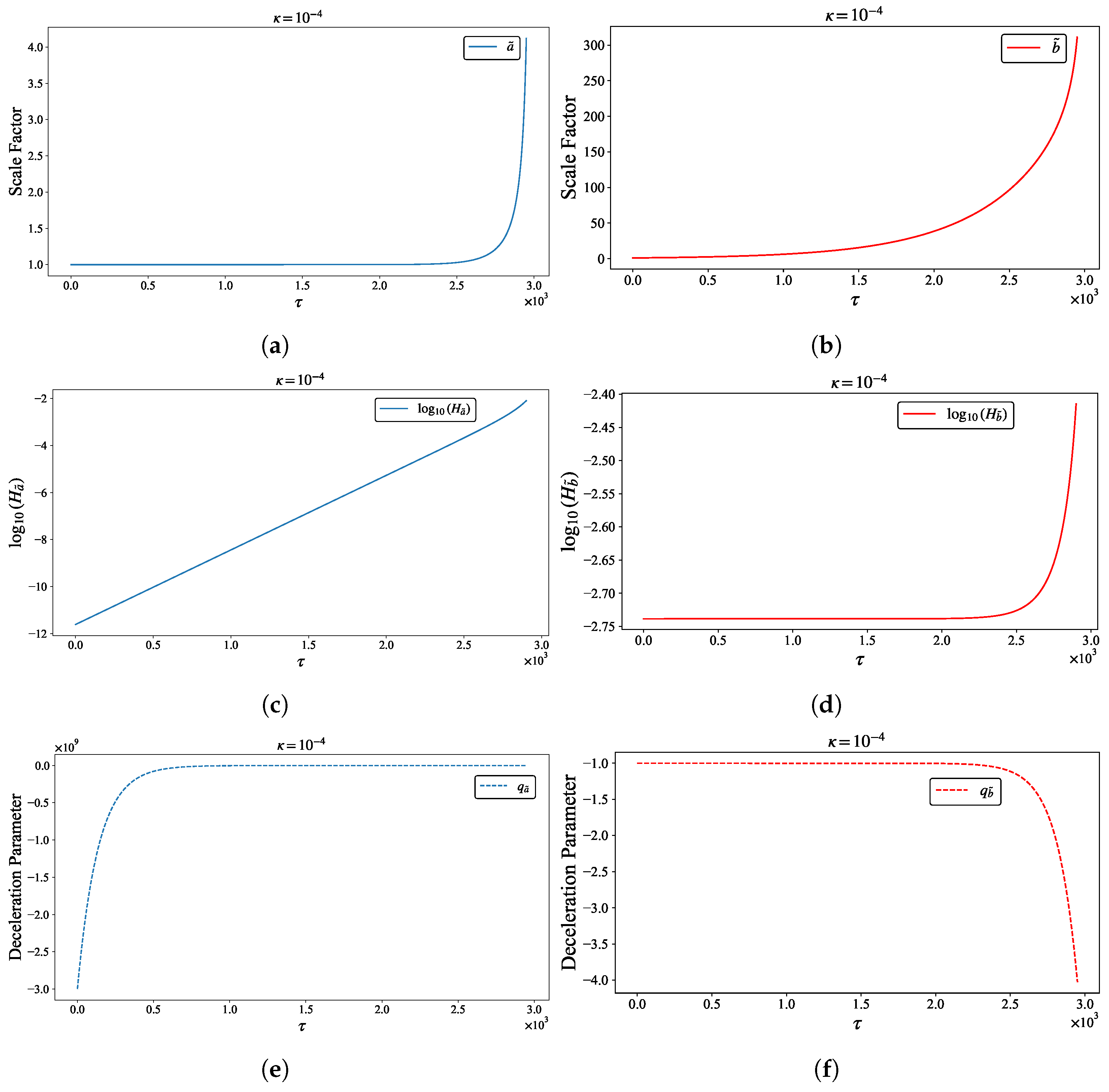
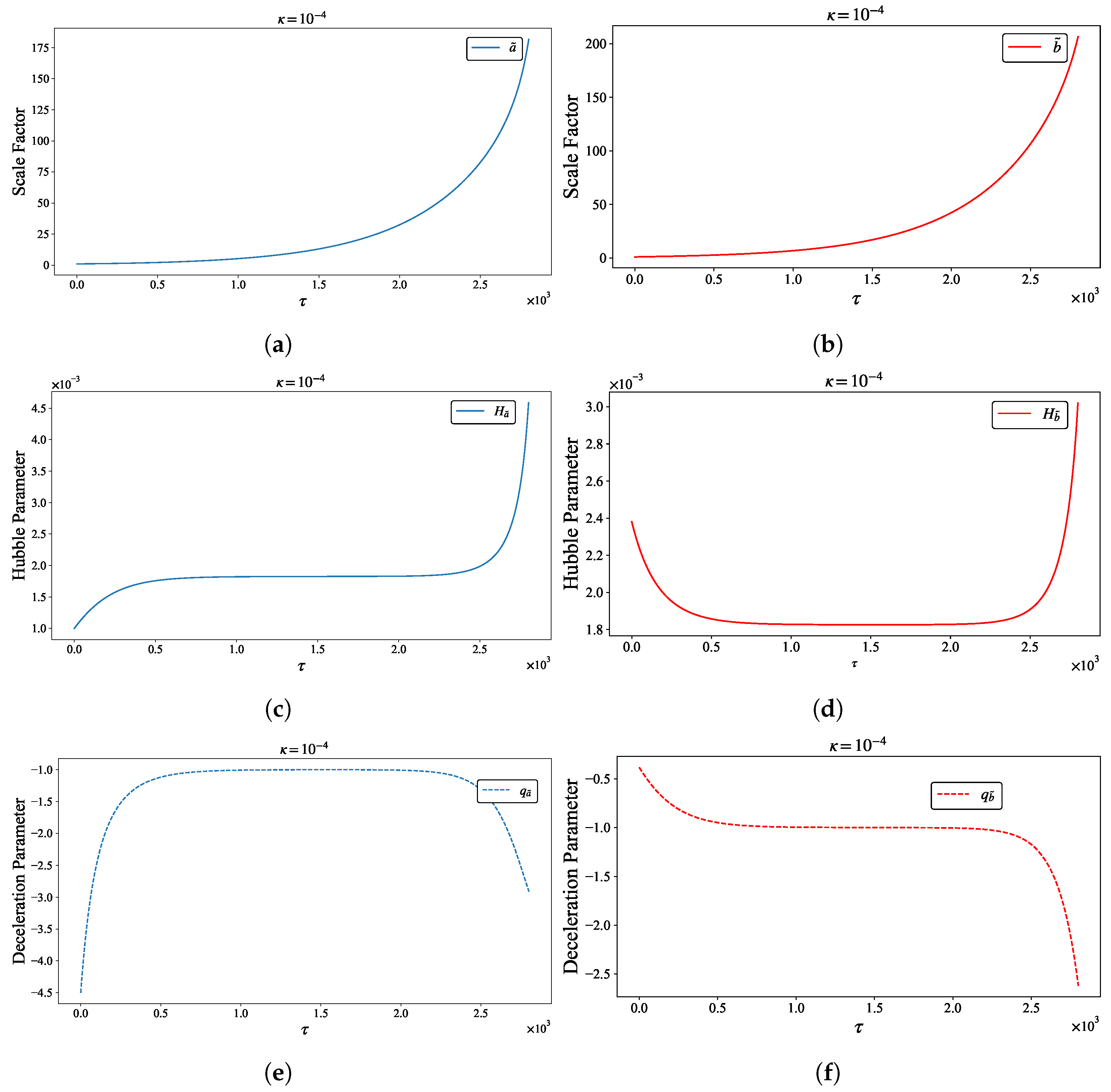
In standard cosmology, a universe with no cosmological constant and in the absence of matter has zero initial momentum. Therefore, the scale factor remains constant during the evolution. In the present GUP-modified dynamics, the situation is different, as depicted in Figure 1.

Several points should be noted. First, regarding the scale factors and Hubble parameter: in patch a, it remains almost constant during most of the evolution (although it is always expanding) and starts to grow rapidly around $\tau$∼2500. In contrast, patch b shows growth consistent with a universe with a non-zero cosmological constant.

The apparent stability of patch $\tilde{a}$ at early times ($\tau <2500$) is due to the scale of the graphs; however, patch a is always expanding. The same observations apply to the Hubble parameter, which exhibits a period of slow growth followed by fast growth at late times.

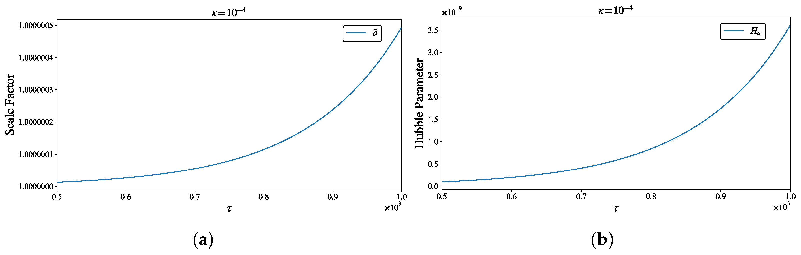
Figure 2 shows the scale factor and Hubble parameter for patch a during the interval $500<\tau <1000$. Over this interval ($\Delta \tau =500$), the scale factor increases by approximately $5\times {10}^{-7}$. By contrast, over a similar time interval at late times ($\tau \gtrsim 2500$), the scale factor grows by ∼4, as shown in Figure 1a. This corresponds to an increase that is roughly ${10}^7$–${10}^8$ times larger. The Hubble parameter exhibits a similar behavior.

In summary, patch a expands from the beginning despite starting with zero momentum and having a vanishing cosmological constant. This behavior arises from the dynamical interaction between the two patches induced by the GUP-inspired deformation of the Poisson algebra.

Sector b also expands, but it contains a non-zero cosmological constant and has non-zero initial momentum. In this case, the GUP effect manifests as explosive growth at late times.

Let us now comment on the results for the deceleration parameter in Figure 1e,f. For sector a (Figure 1e), we observe that it starts from values of $|q_{\tilde{a}}|\sim {10}^9$ and then approaches $|q_{\tilde{a}}|\sim 1$ at late times. In contrast, patch b (Figure 1f) starts at $|q_{\tilde{b}}|\sim 1$ and reaches $|q_{\tilde{b}}|\sim 4$ for late times. The absolute value of $q_{\tilde{b}}$ begins to grow around the same time that the scale factors and Hubble parameters start their rapid growth.

The initial value of $|q_{\tilde{a}}|$ can be traced back to the initial value of the velocity ${\tilde{a}}^{\prime }$. Indeed, substituting the initial values into (12), we obtain

$${\tilde{a}}^{\prime }\left({\tau }_0\right)=\kappa ({\left({\tilde{\pi }}_b\left({\tau }_0\right)\right)}^3+{\lambda }_b{\tilde{\pi }}_b\left({\tau }_0\right)).$$

(22)

From the initial values, it is straightforward to calculate ${\tilde{\pi }}_b\left({\tau }_0\right)$∼$2\times {10}^{-3}$; therefore,

$${\tilde{a}}^{\prime }\left({\tau }_0\right)\approx 3\times {10}^{-12}.$$

Assuming that ${\tilde{a}}^{″}$ is of the same order, a crude approximation for the initial value of $\left|q\right|$ is $q_{\tilde{a}}\left({\tau }_0\right)\approx {10}^{12}$. This estimate is consistent with the order of magnitude observed in Figure 1e.

The behavior of q in the late time period is shown in Figure 3 for patch a in Figure 3a, and for b in Figure 3b.

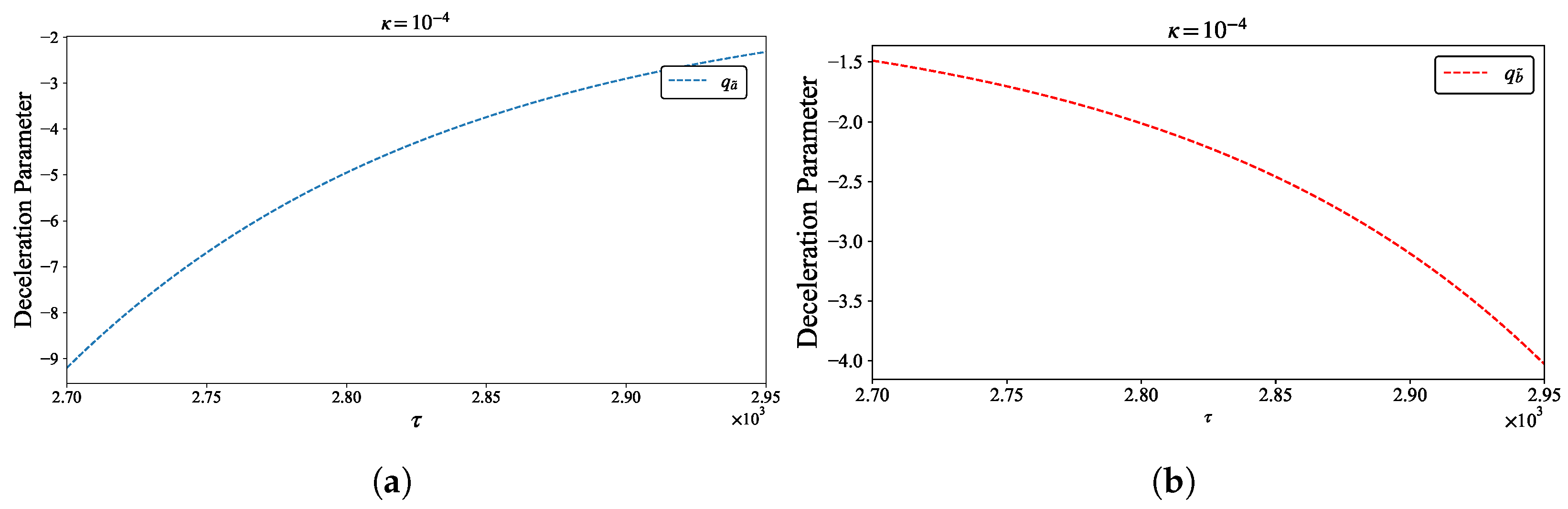
The Figure 3a shows that $q_{\tilde{a}}$ approaches a negative constant asymptotically, indicating positive acceleration. That is, sector a is always accelerating, which is not possible for a universe with ${\lambda }_a=0$ and zero initial momentum. Therefore, the b sector is sourcing this acceleration through the GUP deformation, as it can be seen from Equation (22).

On the other hand, the b sector is also always accelerating, consistent with its non-vanishing cosmological constant there and non-zero initial momentum. Around the time where scale factors and Hubble parameters start their rapid growth, the magnitude of the deceleration parameter ($|q_{\tilde{b}}|$) increases.

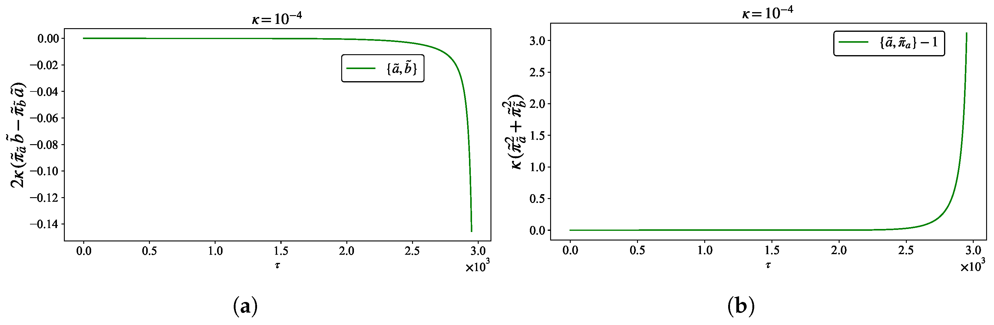
The late-time behavior is explained by the Poisson bracket structure. Indeed, the terms proportional to $\kappa$ (or $\beta$ according to Equation (11)) become more relevant at high momenta, as they depend on $\tilde{\pi }$ and ${\tilde{\pi }}^2$. Figure 4 shows the evolution of these terms, and we can verify that they become significant around $\tau$∼2500, where the rapid growth for the scale factors and the Hubble parameter begins.

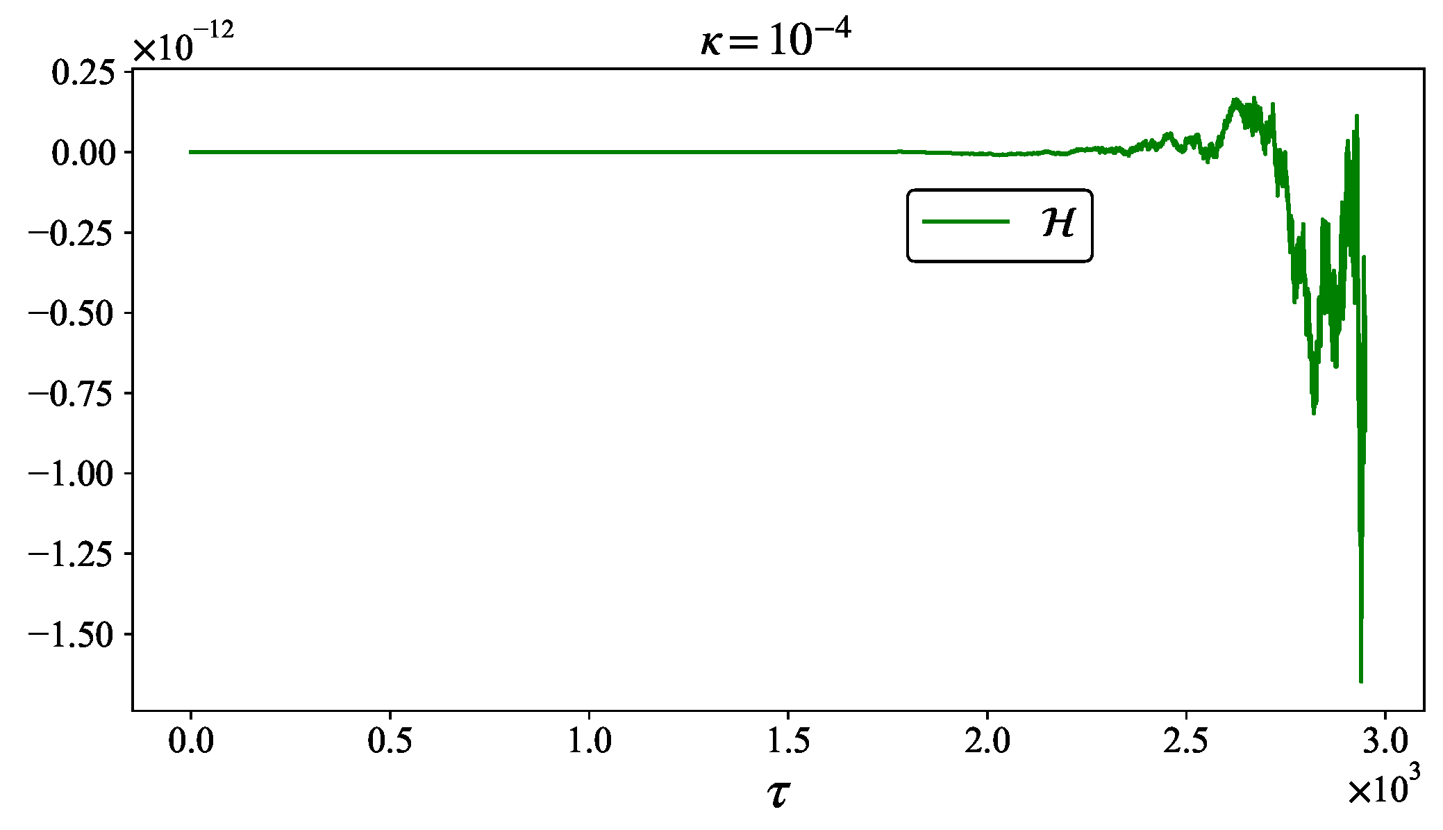
As a final consistency check to rule out possible numerical errors, we verify the Hamiltonian constraint (16), namely, $\mathcal{H}=0$. Figure 5 shows the evolution of this constraint.

It is clear that for large $\tau$, noise (likely from the numerical method) is present; however, it is of the order of ${10}^{-12}$, indicating that this is not responsible for the rapid expansion of the scale factors and Hubble parameters at late times.

These results indicate that the GUP effect in this two-scale-factor model leads to a Big Rip scenario at late times. Even if patch a starts with a zero cosmological constant and zero momentum, the geometry expands so rapidly that the Big Rip appears inevitable at a finite time.

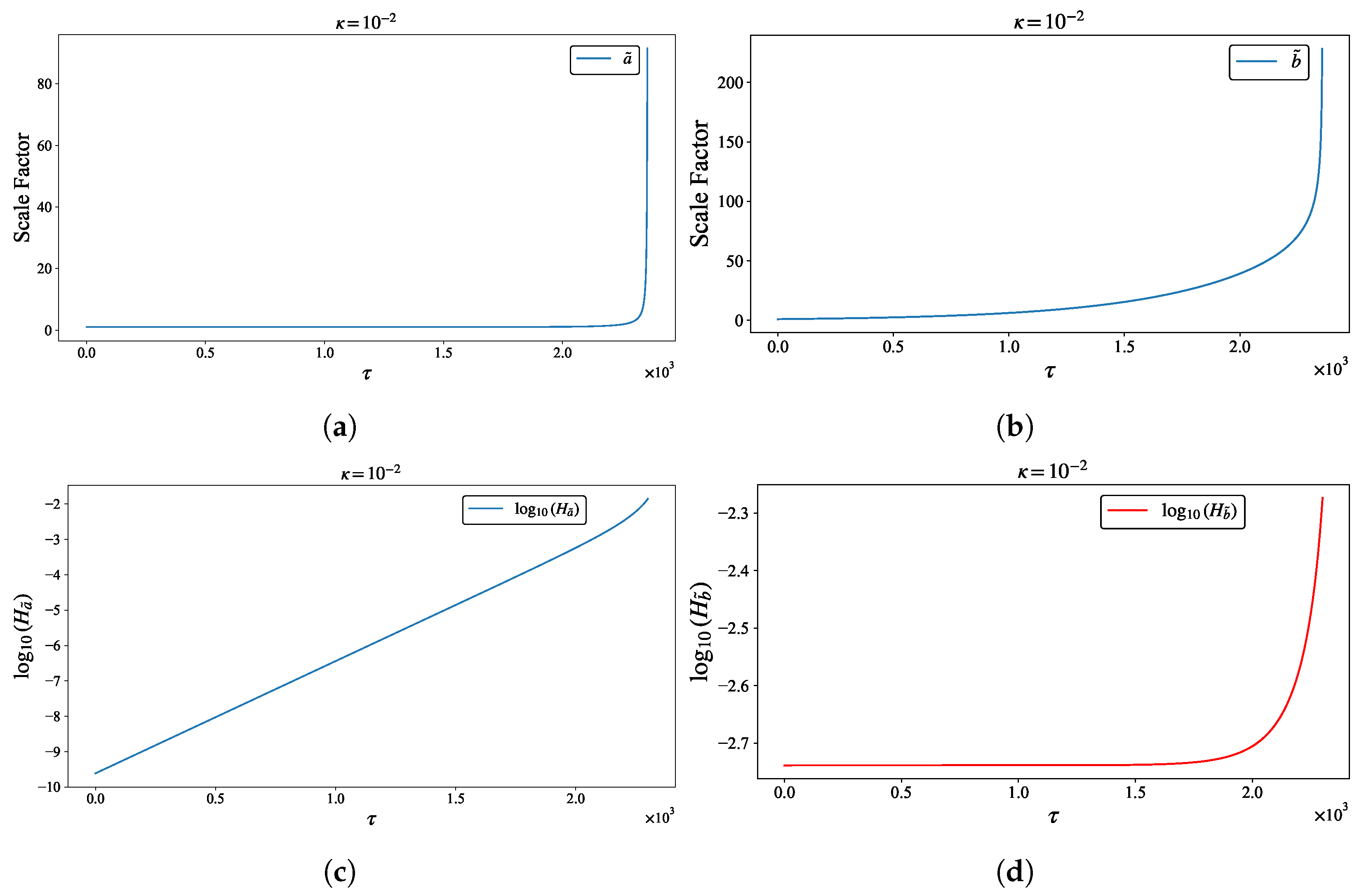
Let us now consider a change in $\kappa$. By taking $\kappa ={10}^{-2}$ (while maintaining ${\lambda }_a=0$, ${\lambda }_b={10}^{-5}$, and ${\tilde{\pi }}_a\left({\tau }_0\right)=0$), the previously discussed effects are expected to appear at earlier times.

Figure 6 illustrates the effects of a larger $\kappa$. As expected, the Big Rip occurs earlier compared to the case where $\kappa ={10}^{-4}$. Furthermore, the accelerated growth occurs closer to the time of the Big Rip.

Now, we explore different initial conditions for both patches with non-zero cosmological constant

3.2. ${\tilde{\pi }}_a\left({\tau }_0\right)\ne 0$ and ${\lambda }_a={\lambda }_b$

This case is interesting since both patches are symmetric. Non-symmetric initial conditions, on the other hand, are relevant as they allow us to determine if the Big Rip can be avoided in one of the patches.

We choose the initial condition ${\tilde{\pi }}_a\left({\tau }_0\right)={10}^{-3}$ (and therefore ${\tilde{\pi }}_b\left({\tau }_0\right)=2.4\times {10}^{-3}$ according to Equation (17)). Note that in this case the maximum initial momentum for sector a is

$${\tilde{\pi }}_a^{\left(\max \right)}=\sqrt{{\displaystyle \frac{2{\lambda }_a}{3}}}=2.6\times {10}^{-3},$$

Thus, we are roughly speaking at a similar distance from the upper and lower bounds of the initial momentum in patch a.

The evolution of both patches for these conditions is shown in Figure 7. The effect in patch a is as expected in the presence of cosmological constant. Compared with the b sector, it is clear that patch b started with higher momentum.

The explosive growth of the scale factor is attenuated; however, the Hubble parameters still exhibit this behavior at late times. This occurs at approximately the same time as in the case discussed in the previous section.

Deceleration parameters show again that the final stage for both patches is one of increasing acceleration. Moreover, there is a time interval where both patches behave as de Sitter universes (with $q=-1$); however, towards the end of the evolution, $\left|q\right|$ increases and the integration stops at a finite time, which is consistent with the Big Rip scenario.

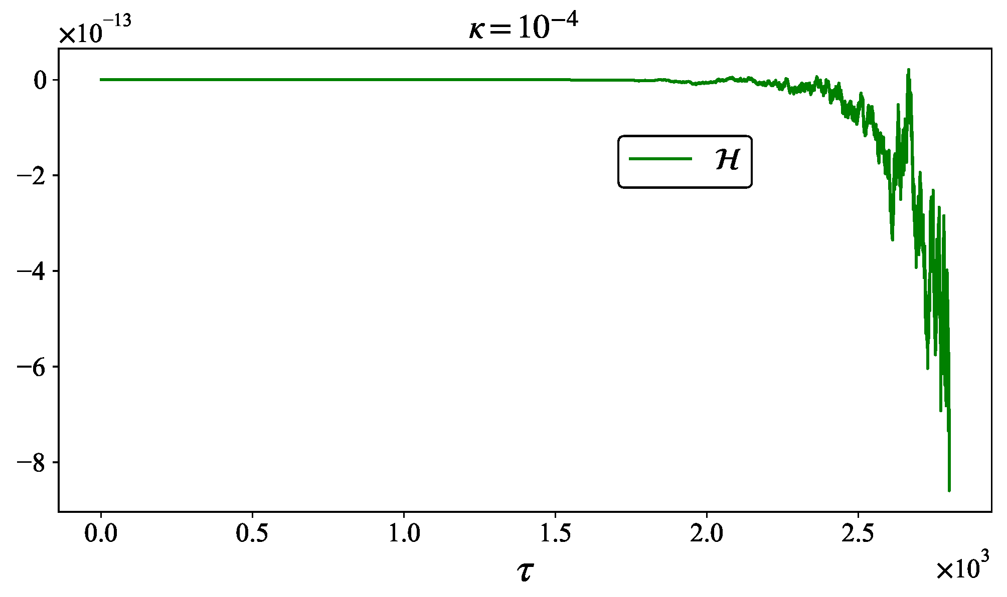
Let us complete the discussion by verifying the Hamiltonian constraint. For this set of initial conditions, the constraint is shown in Figure 8. It is clear that any significant numerical error can be safely excluded.

The next question we would like to address concerns the robustness of this behavior. Specifically, the Big Rip observed here depends strongly on the deformation parameter. Is it possible to link $\kappa$ to the time at which the accelerated growth occurs? This is the primary objective of the next section.

4. Scaling Laws and the Rip Time

Our objective is to determine the values of $\tau$ at which our numerical analysis can no longer proceed, starting from a fixed initial ${\tilde{\pi }}_a$ and given values of ${\lambda }_a$ and ${\lambda }_b$.

The strategy consists of numerically solving the equations of motion and identifying the value of $\tau$ where any of the following conditions are met: (a) the scale factors or momenta reach an undefined value; or (b) the Hubble parameter reaches a specific threshold. In the present case, this threshold was set to $H_{th}=300$.

If either condition was satisfied, the simulation recorded the critical time T for the specific $\kappa$ under consideration. Beyond that value of T no finite solution of the equations of motion was found. The parameter sweep was performed for $\kappa$ values ranging from ${10}^{-7}$ to ${10}^{-1}$ following a 1-5-10 logarithmic stepping.

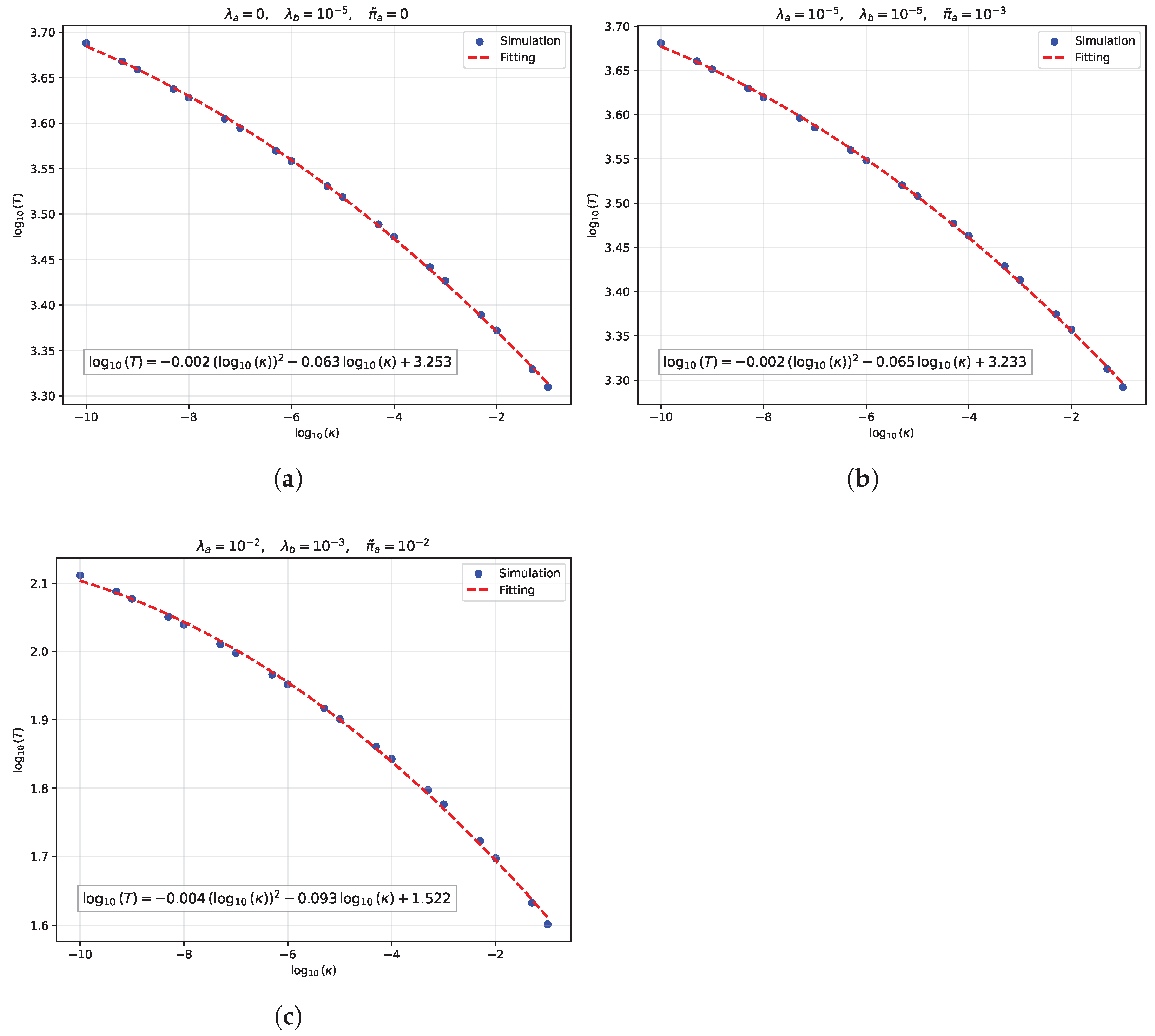
The best fit found in our analysis was

$${\log }_{10}\left(T\right)=A{\left({\log }_{10}\kappa \right)}^2+B{\log }_{10}\kappa +C.$$

(23)

The results for the cases previously discussed are presented in Figure 9. Figure 9c illustrates a scenario not yet addressed in our analysis; however, these results indicate that for the given cosmological constants and initial momentum ${\tilde{\pi }}_a$, the evolution terminates in a divergence of the scale factors and the Hubble parameter. This occurs at a critical time T, as shown in the plot for each value of $\kappa$.

5. Negative $\mathit{\kappa }$

This section is devoted to analyzing the case of $\kappa <0$. In the GUP proposal, this scenario yields no minimal-length scale, but here, in this classical theory, no restriction is found.

From (21), we see that for ${\mathit{\pi }}^2=\left|{\kappa }^{-1}\right|$, a negative value of $\kappa$ implies $\{\tilde{a},{\tilde{\pi }}_a\}=0$, rendering a degeneration in the symplectic structure. In this sense, the system is no longer Hamiltonian.

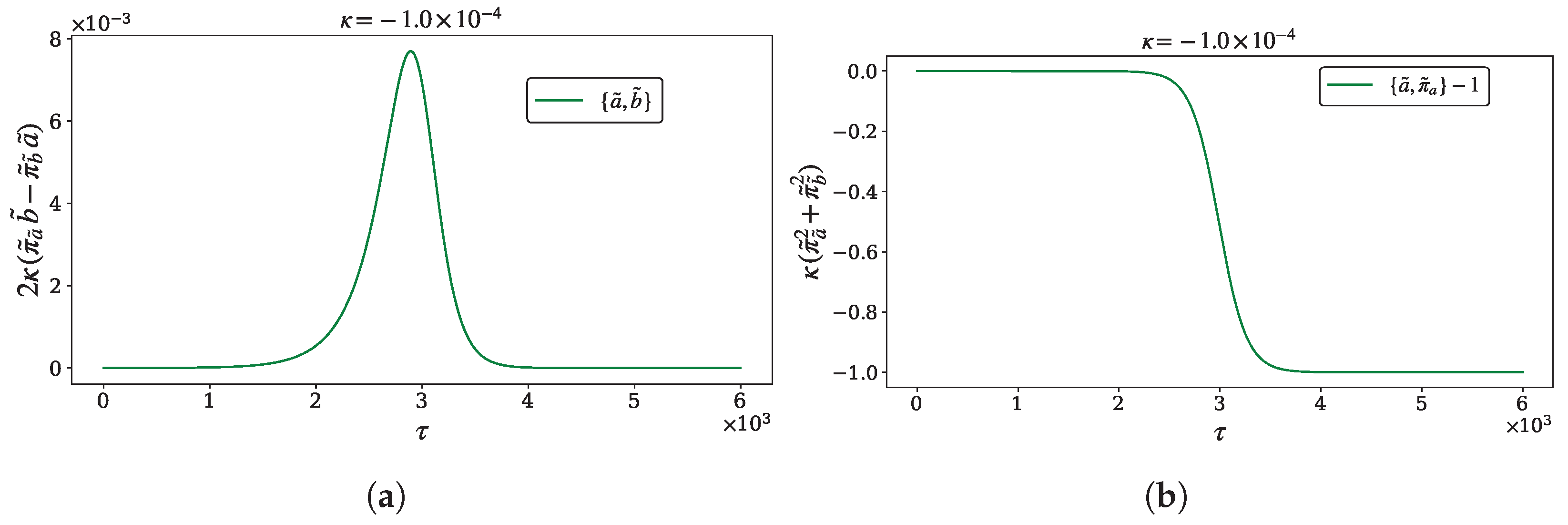
Figure 10 shows the evolution of the modified part of the Poisson brackets for the initial conditions ${\tilde{\pi }}_a\left({\tau }_0\right)=0$, and cosmological constants ${\lambda }_a=0$, and ${\lambda }_b={10}^{-5}$.

The GUP deformation on $\{\tilde{a},\tilde{b}\}$ remains nearly zero, only reaching the order of ${10}^{-3}$ for a finite duration. During that interval, the deformation on $\{\tilde{a},{\tilde{\pi }}_a\}$ transitions from approximately one to zero, representing the transition period toward a degenerate symplectic structure.

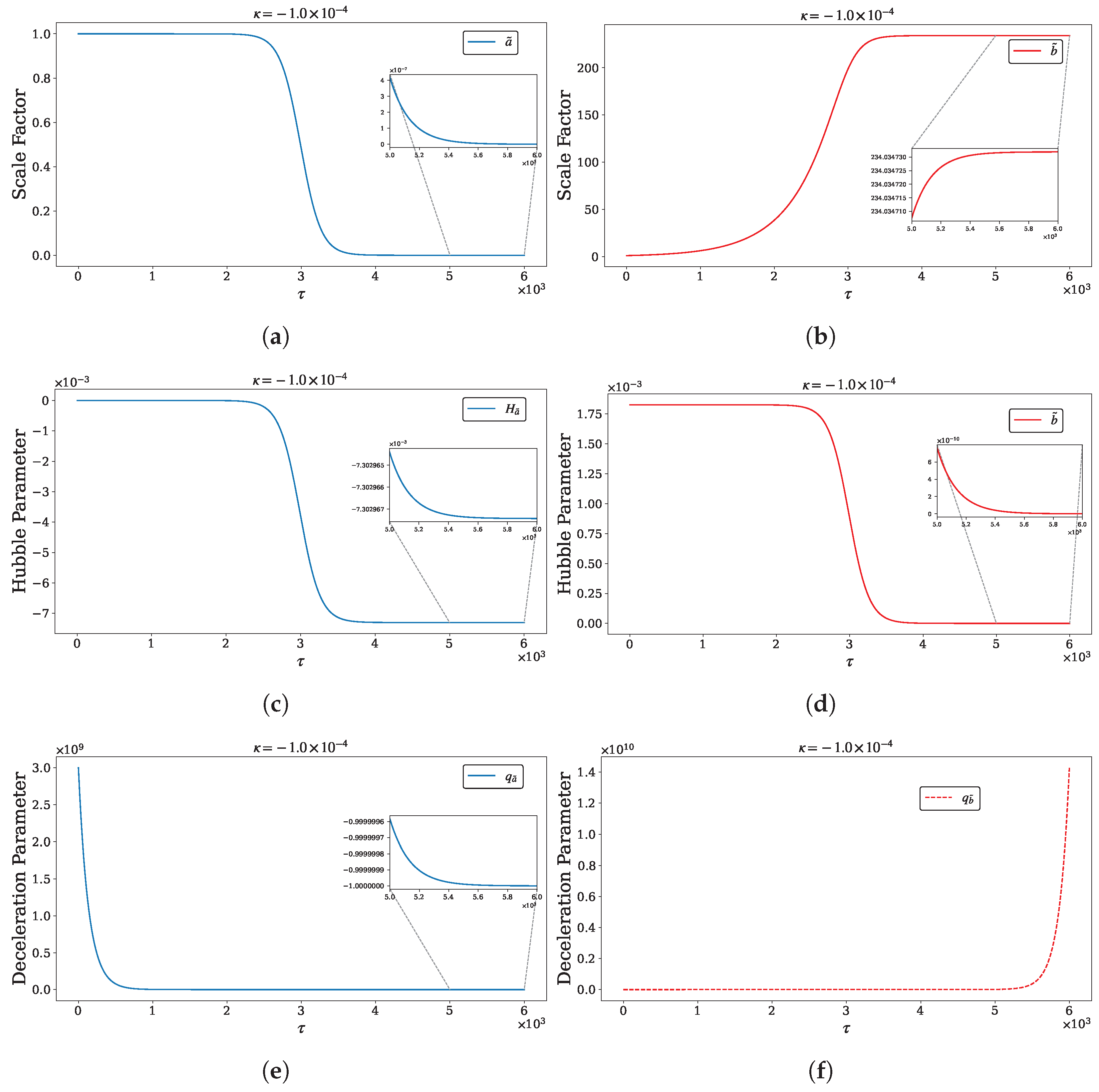
The impact of this deformation on the evolution of the scale factor and the Hubble parameter is illustrated in Figure 11. For $\tau \gtrsim 5000$, corresponding to the regime where $\{\tilde{a},{\tilde{\pi }}_a\}$∼0∼$\{\tilde{b},{\tilde{\pi }}_b\}$, the scale factor a approaches zero, causing the patch to shrink, while the scale factor b converges to a non-zero constant value.

Regarding patch a, Figure 11c shows that the Hubble parameter tends toward a negative value (as seen in the inset zoom); consequently, the scale factor undergoes exponential contraction. This asymptotic contraction is clearly visible in the zoom of Figure 11a. Furthermore, the deceleration parameter must approach $-1$ in this scenario, which is confirmed by Figure 11e and its corresponding inset.

A similar analysis applies to sector b; however, in that case, the scale factor freezes at a finite value, causing the Hubble parameter to subsequently vanish. The deceleration parameter diverges as the expansion velocity approaches zero. These results can be verified in Figure 11b,d.

For different values of $\lambda$ and initial conditions, the behavior is similar. That is, once the system becomes a degenerated symplectic one, one patch shrinks, while the other freezes. That is, a negative $\kappa$ changes drastically the fate of the patches.

A final comment regarding this behavior: Clearly, as $\{\tilde{a},{\tilde{\pi }}_a\}\to 0$ (as well as the variables on patch b), the symplectic structure becomes singular, and our previous conclusions must be taken cautiously. That is, we cannot go further with the evolution for later times.

The next section summarizes our results and discusses possible routes to investigate.

6. Conclusions and Discussion

In this work we studied the evolution of a bi-metric universe with a classical GUP Poisson bracket structure. The two scale factors might represent two patches of the universe which are, in principle, causally disconnected, or a multiverse scenario.

This model of gravity has been analyzed in previous works in the context of deformed Poisson structures inspired by non-commutative models. In the present work, the approach is based on possible effects of a Quantum Gravity theory (namely the GUP proposal) at the classical level, and therefore on a non-standard Poisson bracket.

Those Poisson brackets, unlike those inspired by non-commutative models, have extra terms which depend on dynamics through the momenta of the fields. This suggests that the effects of the deformation might be important at high momentum, even though these terms are proportional to the parameter of the deformation which can be small.

The numerical analysis showed that behavior. Indeed, the scale factor evolution, as well as the Hubble parameters in both patches, exhibited explosive growth at late times. The deceleration parameter confirmed that the universe was always accelerating.

The time at which such expansion becomes critical depends on the deformation parameter and the initial conditions. We showed that for two very different cases (one with ${\tilde{\pi }}_a\left({\tau }_0\right)=0,{\lambda }_a=0$, and the other with ${\tilde{\pi }}_a\left({\tau }_0\right)={10}^{-3},{\lambda }_a={\lambda }_b={10}^{-5}$) the scale factors and the Hubble parameter reached a maximum value beyond which it was no longer possible to determine the evolution of the system.

As the evolution approached that point, the acceleration did not stop. An analysis of the Hamiltonian constraint’s behavior allowed us to dismiss the possibility that this effect arose from purely numerical origin.

The possibility that this effect is a particular result of the chosen values of initial conditions and cosmological constants can also be dismissed. The power-law relation between the deformation parameter and the lifetime of the patches (that is, the time T in Figure 9a,b, beyond which the system can no longer be integrated) shows that the Big Rip occurs earlier for larger $\kappa$’s.

The origin of this effect in this particular form of the GUP is precisely the deformation term of the Poisson bracket structure. Its proportionality to the momenta of the fields makes the effects of the deformation important for later times, and therefore, for high momenta. Clearly, small values of $\kappa$ make this effect important for late times.

A completely different scenario develops for $\kappa <0$. Here, since the Poisson bracket deformation is dynamical, the symplectic structure becomes degenerate at a finite time. Here, the Hamiltonian dynamics is no longer valid since $\{a,{\tilde{\pi }}_a\}\to 0$. The asymptotic behavior of the patches shows that, as the time approaches that end, one of the patches shrinks while the other remains frozen.

Clearly, this singularity is reached at a finite time $\tau ={\tau }_{\mathrm{crit}}$, for which ${\tilde{\pi }}_a^2\left({\tau }_{\mathrm{crit}}\right)+{\tilde{\pi }}_b^2\left({\tau }_{\mathrm{crit}}\right)=1/\left|\kappa \right|$. Beyond that time, the dynamics require a different approach. In this sense, the conclusion of a frozen sector and a shrinking sector deserves careful analysis that goes beyond the scope of present work.

Nonetheless, this might be a concrete dynamical mechanism that ends the connection between patches. We can speculate, then, that this GUP mechanism—a remnant of a quantum gravity—affects the evolution of patches at initial times and, at some finite time, the action ceases. From there, the evolution of one of the patches follows the standard evolution.

All the previous analysis is valid in the absence of matter. The presence of matter offers the possibility of delaying the Big Rip scenario in the case of $\kappa >0$, due to the attraction that matter introduces. Results involving the presence of matter will be presented elsewhere in the near future.