Article

Bayesian Inference of Primordial Magnetic Field Parameters from CMB with Spherical Graph Neural Networks


by
Juan Alejandro Pinto Castro
1,
Héctor J. Hortúa
1,2,*,
Jorge Enrique García-Farieta
1 and
Roger Anderson Hurtado
3
1
Laboratorio de Inteligencia Artificial (SavIA Lab), Grupo Signos, Departamento de Matemáticas, Universidad El Bosque, Bogota 111321, Colombia
2
Instituto de Neurociencias, Universidad El Bosque, Bogota 111321, Colombia
3
Observatorio Astronómico Nacional, Universidad Nacional de Colombia, Bogota 110911, Colombia
*
Author to whom correspondence should be addressed.
Universe 2026, 12(2), 34; https://doi.org/10.3390/universe12020034
Submission received: 21 October 2025 / Revised: 16 January 2026 / Accepted: 20 January 2026 / Published: 26 January 2026
(This article belongs to the Section Astroinformatics and Astrostatistics)

Abstract

Deep learning has emerged as a transformative methodology in modern cosmology, providing powerful tools to extract meaningful physical information from complex astronomical data. This paper implements a novel Bayesian graph deep learning framework for estimating key cosmological parameters in a primordial magnetic field (PMF) cosmology from simulated Cosmic Microwave Background (CMB) maps. Our methodology utilizes DeepSphere, a spherical convolutional neural network architecture specifically designed to respect the spherical geometry of CMB data through HEALPix pixelization. To advance beyond deterministic point estimates and enable robust uncertainty quantification, we integrate Bayesian Neural Networks (BNNs) into the framework, capturing aleatoric and epistemic uncertainties that reflect the model confidence in its predictions. The proposed approach demonstrates exceptional performance, achieving R 2 scores exceeding 89% for the magnetic parameter estimation. We further obtain well-calibrated uncertainty estimates through post hoc training techniques including Variance Scaling and GPNormal. This integrated DeepSphere-BNNs framework delivers accurate parameter estimation from CMB maps with PMF contributions while providing reliable uncertainty quantification, enabling robust cosmological inference in the era of precision cosmology.

1. Introduction

Cosmic Microwave Background (CMB) radiation is a cornerstone of modern cosmology as it provides a snapshot of the physics of the early Universe [1]. The CMB is sensitive to physical densities because the evolution of acoustic oscillations in the primordial plasma depends directly on them, rather than merely on their fractional contribution to the total energy density [2]. Precise estimation of key cosmological parameters, such as the physical baryon density ω b , cold dark matter density ω c , reionization optical depth τ , scalar spectral index n s , the amplitude of the primordial power spectrum A s , and Hubble parameter H 0 , is essential for understanding the composition and evolution of the Universe. In particular, the Hubble parameter, which describes the expansion rate of the Universe, has garnered significant attention due to the so-called Hubble tension [3,4]. This term refers to a persistent and statistically significant discrepancy between the values derived from independent cosmological measurements of the early Universe and those obtained from local data [5]. Primordial magnetic fields (PMFs) [6,7] offer a potential solution to the Hubble tension that is not inherently fine-tuned for that purpose. Previous studies, such as [8,9,10], have shown that PMFs can induce baryon inhomogeneities, which accelerate the recombination process and consequently increase the CMB-inferred value of H 0 , bringing it into closer agreement with local measurements. The PMF scenario is particularly compelling because it is grounded in well-established theoretical frameworks that predate the Hubble tension and have long been investigated as a possible origin of the large-scale magnetic fields observed in galaxies and clusters; see, e.g., [11,12,13].
Beyond their potential role in addressing cosmological tensions, PMFs serve as valuable probes of early-Universe physics. They are motivated by high-energy processes, such as inflationary magnetogenesis and cosmological phase transitions [14,15,16,17]. As such, constraints on PMFs derived from CMB observations offer a promising avenue for investigating the origin and evolution of cosmic magnetism, while also providing natural predictions in certain extensions of the Standard Model [18]. Furthermore, PMFs imprint distinct signatures on the CMB by sourcing scalar, vector, and tensor perturbations, thereby modifying both temperature and polarization anisotropies [19]. PMFs can generate vector modes and B-mode polarization patterns that are absent in the standard Λ CDM model, as well as induce Faraday rotation of the CMB polarization plane [20], producing a frequency-dependent signal that upcoming experiments, such as the Simons Observatory, LiteBIRD, and CMB-S4, aim to detect [21].
On the other hand, the choice of inference methodology and statistical framework is a critical determinant of the precision and reliability of constraints on cosmological parameters or PMF models [22]. Robust bounds depend on the accurate modeling of the likelihood, thorough treatment of systematics, well-motivated priors, and a careful handling of parameter degeneracies. In addition, traditional techniques applied to the power spectrum are computationally expensive and may not fully exploit the non-Gaussian information present in the CMB maps. This creates a compelling opportunity for deep learning techniques to provide faster and potentially more accurate estimates by learning directly from high-resolution maps [23].
A primary challenge in applying standard deep learning architectures to CMB analysis is the data’s inherent spherical geometry. Conventional convolutional neural networks, designed for flat grids, introduce distortions and are ill-suited for processing data on the sphere. From that perspective, this work is intended to address this issue using the spherical convolutional neural network DeepSphere [24,25,26]. DeepSphere uses a pixelation scheme to represent spherical data, called HEALPix [27], which divides the sphere into pixels of equal area in a hierarchical way, allowing the neural network to efficiently perform convolutions and analysis of the celestial sphere [28].
Beyond geometric challenges, robust inference requires not only accurate predictions but also reliable uncertainty quantification. Standard deep learning models provide deterministic point estimates, failing to capture the epistemic uncertainty associated with limited data or model limitations. To this end, we integrate Bayesian Neural Networks (BNNs) [29] into our architecture. BNNs learn a probability distribution over the model weights, naturally quantifying predictive uncertainty.
This work is organized as follows: Section 2 provides background on graph neural networks, DeepSphere, and Bayesian Neural Networks. Section 3 details our methods, including the simulation pipeline, data validation, network architecture, and training procedure. Section 4 presents the results and analysis of the model’s performance and uncertainty calibration. Finally, Section 5 and Section 6 conclude the paper and discuss future research directions.

2. Neural Networks

Deep learning has become an essential tool in modern cosmology, transcending the limitations of traditional statistical methods to address the challenges posed by the massive, complex, and high-dimensional nature of CMB [30,31,32]. This research leverages convolutional operations extended to graph neural networks to predict cosmological parameters; specifically, we use the DeepSphere framework [24]. DeepSphere offers an efficient implementation of spherical convolutions by representing the celestial sphere as a graph and performing spectral or spatial graph convolutions, thus preserving the global geometry of the CMB data. Furthermore, we use the Bayesian Neural Networks approach, which learn the mean and variance to define a probability distribution over the weights. This approach explicitly quantifies epistemic uncertainty, reflecting the model’s confidence in its predictions arising from limited data or inherent model limitations [29,33].

2.1. Graph Neural Networks and DeepSphere

Graph neural networks (GNNs) are a class of supervised deep learning models [34] which can learn functions over graphs and are a leading approach for building predictive models on graph-structured data G ( V , E ) [35], where nodes V are objects interconnected by edges E , which are relationships [36]. GNNs represent a formidable progression in deep learning, designed to process data structures in non-Euclidean domains where Convolutional Neural Networks (CNNs) have limitations [37,38]. The success of GNNs in handling arbitrary relational data has led to the broader field of geometric graphs, which aims to generalize deep learning operations to diverse non-Euclidean manifolds [39]. In some domains, the nodes in the graph are embedded in a 3D space; therefore, the coordinates could be used as features of the nodes [35]. In cosmology, objects like dark matter halos and galaxy clusters are represented as nodes connected by edges that trace cosmic filaments and spatial proximity [34]. When working with geometrical graphs, it is important to consider the symmetry of the task with respect to translations and rotations of the frame of reference [35], and to generalize data defined on a curved surface, such as CMB maps with PMFs and weak lensing. The challenge is to develop a method that respects spherical symmetry [30]. This challenge drives the development of Spherical Convolutional Neural Networks (SCNNs) such as DeepSphere (https://github.com/deepsphere (accessed on 19 January 2026)) [24,25,26], which is computationally efficient and well adapted to the spherical geometry of the CMB. This adaptation is essential because the CMB is naturally represented on the two-sphere, S 2 , and is typically pixelized using the HEALPix scheme [27]. The HEALPix pixels are treated as nodes of a graph, and local neighborhoods are exploited through spherical convolutions defined directly on the pixelization. With many standard CNN operations, such as convolutions and pooling, using filters restricted to being radial, DeepSphere can be made invariant or equivariant to rotation. This ensures that the extracted features are independent of the map’s orientation, a necessary constraint for robust inference. DeepSphere has been shown to be computationally more efficient than harmonic-based methods and yields superior performance in tasks such as cosmological model discrimination, particularly in scenarios involving high noise levels or partial sky coverage, confirming its utility for next-generation surveys [24].

2.2. Bayesian Neural Networks

Standard deep learning models are characterized by their deterministic nature, learning single-point estimates for all model parameters. While it is effective for prediction, those models fail to quantify the epistemic uncertainty inherent in the data and prediction process, a critical requirement for robust scientific inference [40]. Bayesian Neural Networks offer a principled approach to quantifying uncertainty in deep learning models. They treat the model parameters as random variables governed by probability distributions, thereby capturing epistemic uncertainty [41]. Inference in BNNs involves computing the posterior distribution, p ( w | D ) , over the weights, w , given the training data D . This is commonly achieved via scalable methods such as variance inference or Monte Carlo Dropout [29,33]. Variance inference is the preferred and scalable method for training BNNs, which finds a distribution q ( w | θ ) that minimizes the difference to the true posterior p ( w | D )  [41] as well as a prior distribution on the weights p ( w ) . This step is reached by minimizing the KullBack–Leibler (KL) divergence between the two distributions, and is equivalent to maximizing the evidence lower bound (ELBO) [29], which includes a term associated with the negative log-likelihood (NLL), as [31]
ELBO KL NLL = KL ( q ( w | θ ) | | p ( w ) ) ( 1 2 log | Σ | + 1 2 ( y μ ) T Σ 1 ( y μ ) ) ,
where Σ is the predicted covariance matrix, y is the observed data, and μ is the predicted mean vector of the model. The application of BNNs to the estimation of cosmological parameters has been investigated in recent works [31,32]. The combination of GNNs and BNNs results in a powerful framework, which not only achieves high predictive accuracy but crucially reliable estimates of epistemic uncertainty.

3. Methods

To analyze the simulated CMB with PMF maps and extract cosmological information, we employed DeepSphere, a graph-based convolutional neural network architecture specifically designed for spherical data [24]. Specifically, we make use of the HealpyPseudoConv layers, which implement convolution operations on the sphere by aggregating information from neighboring pixels according to the hierarchical structure of HEALPix. In addition, we employ HealpyPooling layers, which perform a coarsening of the sphere by reducing the resolution defined by nside. This combination of spherical convolution and pooling layers allows the network to efficiently capture both large-scale and small-scale anisotropy patterns of the CMB, while remaining computationally feasible for high-resolution data. Compared to planar projections, the spherical approach has the advantage of avoiding distortions and preserving the isotropy of the signal, which is crucial for cosmological inference tasks [27]. In cosmological applications, DeepSphere has been applied to tasks such as weak lensing map classification, cosmological parameter estimation, and non-Gaussianity detection [24]. In our study, we extend its use to the problem of predicting five cosmological parameters—the cold matter density ω c , the baryon density ω b , the amplitude A s , the amplitude of the PMF B 1 Mpc , and the magnetic damping scale relation β = log 10 ( τ ν / τ B ) , including PMF contributions directly from simulated CMB maps.

3.1. Simulation of CMB Maps with PMF

We generated CMB temperature and polarization anisotropy maps using a modified pipeline based on CAMB (https://camb.info/ (accessed on 19 January 2026)) [42,43], specifically, the patch for CAMB that computes CMB sourced by PMFs [22,43], and Healpy (https://healpix.sourceforge.io/ (accessed on 19 January 2026)) [27]. The latter was used to pixelize and manipulate the spherical CMB maps and to generate random CMB realizations in Healpix format from the input power spectrum. Following the implementation in [22], CAMB is modified to incorporate the effects of PMFs by treating them as a stochastic, non-helical Gaussian field. The implementation follows a covariant formalism where the magnetic energy–momentum tensor acts as an active source in the linear Einstein–Boltzmann equations. Specifically, the code accounts for scalar, vector, and tensor contributions, scaling the comoving magnetic field as B a 2 under the ideal MHD approximation. To ensure physical consistency, the patch recalculates the correlation functions for a power-law spectrum P B ( k ) k n B including an ultraviolet cutoff at the damping scale k D and explicitly adds both passive and compensated magnetic modes (generated before and after neutrino decoupling). Furthermore, the code employs asymptotic approximations for the convolution integrals to maintain numerical stability across different spectral index regimes. As a result, this CAMB’s variant generates the full set of angular power spectra (TT, EE, BB, and TE), where the PMF-induced vector and tensor modes provide distinct signatures, particularly in the BB-mode signal at high multipoles. These spectra are then passed to Healpy, which synthesizes them into simulated full-sky CMB maps in the form of Stokes I, Q, and U parameters. This framework incorporates standard Λ CDM physics and assumes a flat Universe. It is restricted to three massless neutrinos and passive, compensated magnetic modes that are mutually uncorrelated [22]. In addition, we assume that primordial magnetic fields were generated within the simplest inflationary magnetogenesis scenario. Under this model, the magnetic spectral index naturally approaches the nearly scale-invariant value n b = 2.9 [44]. The total theoretical angular power spectrum is given by
C l theor = C l prim + C l pass + C l comp ,
comprising three main components: the primordial (non-magnetic) spectrum from standard cosmological perturbations C l prim , the passive magnetic contribution C l pass , and the compensated magnetic contribution C l comp . Scalar perturbations are presented in both the compensated C l comp and passive C l pass modes; vector perturbations are included in the compensated contribution C l comp and tensor perturbations are included in the passive contribution C l pass (more details in Appendix A.3). In this paper, we adopt the following notation: full to refer to the dataset including scalar, vector, and passive magnetic contributions, and prim-vp to refer to the dataset excluding the scalar compensated mode. Two independent datasets were constructed, each containing 1000 power spectra with 5 realizations, so that each dataset, full and prim-vp, contains 5000 maps. The cosmological parameters were set to Planck best-fit cosmology [45], with  h = 0.67556 , which is the dimensionless reduced Hubble constant, defined as h = H 0 / 100 ( kms 1 Mpc 1 ) , the scalar spectral index n s as 0.9665 , and the magnetic spectral index n B as 2.9 . Table 1 summarizes the ranges of cosmological and primordial magnetic field (PMF) parameters used in the generation of the datasets used in this study. These parameters span values chosen to cover the relevant physical scenarios considered in our analysis.
Table 1 summarizes the cosmological and PMF parameters adopted for dataset generation, along with the corresponding reference values from the Planck best-fit Λ CDM cosmology [45]. We selected prior ranges significantly wider than the current tight constraints from the Planck mission. This choice allows us to test the robustness and generalization of our neural network: by training over a large parameter volume, the model learns the underlying physical relationships between cosmological parameters and the CMB maps rather than overfitting to a narrow region near the current best-fit values. Such an approach is common in early-stage machine learning applications for cosmology. The PMF-related parameters, B 1 Mpc and β , extend beyond the standard Λ CDM framework. However, according to Plank results: constrains on primordial magnetic field (2015) [46] and Zucca et al. [22], representative values of B 1 Mpc = 5 nG and β = 17 were used in their analysis of PMF-induced anisotropies, which lie close to the upper and lower limits of the ranges explored in this study.

3.2. Dataset and Validation

The CMB is modeled as a Gaussian random field, meaning that it is not a unique deterministic sky but a statistical ensemble of possible realizations, all of them characterized by the same angular power spectra C l . While most values in these realizations cluster near the mean, a finite number of modes in the sky, especially at large angular scales where cosmic variance is high inevitably, leads to extreme fluctuations. These statistically plausible outliers are a natural consequence of cosmic variance [45]. The broad parameter ranges chosen for dataset generation (see Table 1) were adopted following the analysis in [22], where they investigated constraints on PMF from Planck mission and South Pole Telescope data. Their choice of ranges is motivated by both observational and theoretical considerations. The damping scale ratio ( β = log 10 ( τ ν / τ B ) ), for instance, can capture a variety of physically plausible PMF generation scenarios, including inflationary and phase-transition models. Standard cosmological parameters such as ω c , ω b , and A s were also varied within extended ranges compared to Planck priors. This approach is essential for exploring degeneracies between PMF effects and baseline cosmology. Furthermore, we implemented a data-cleaning procedure to remove maps with pixel values outside physically reasonable limits. The minimum and maximum pixel values of each image were examined, and a per-pixel threshold criterion was applied to flag anomalous maps. Maps exceeding these thresholds were classified as outliers and excluded from the dataset. Similar pre-processing and anomaly-rejection strategies have been employed in recent works applying deep learning to CMB data, ensuring robust inference of cosmological parameters [47]. We found extreme outliers in some maps with magnitudes up to 10 30 , which are effectively removed after thresholding, resulting in a clean and coherent data range below 10 6 (more details in Appendix A.2). From the initial 5000 CMB maps generated with CAMB, full reaches 67 anomalous maps discarded, leaving 4933 valid maps, and prim-vp reaches 83 anomalous maps discarded, leaving 4917 valid maps. The cleaned dataset was randomly partitioned into training, validation, and test subsets using a two-step procedure. First, 70 % of the data was allocated to the training set, while the remaining 30 % was reserved for further splitting. This reserved portion was then evenly divided into validation and test sets, each comprising 15 % of the original dataset. In addition, we generated an independent dataset consisting of 400 simulated CMB maps with one realization, which serves as an external validation set for the model. This dataset was built under the same physical assumptions as the training data but with a distinct random seed. The main purpose of this external dataset is to evaluate the generalization capacity when exposed to unseen data distributions [48]. With this, the test dataset measures the model’s generalization during training, the validation dataset monitors overfitting and manages hyperparameter tuning, and the external dataset assesses generalization to unseen data.

3.3. Architecture

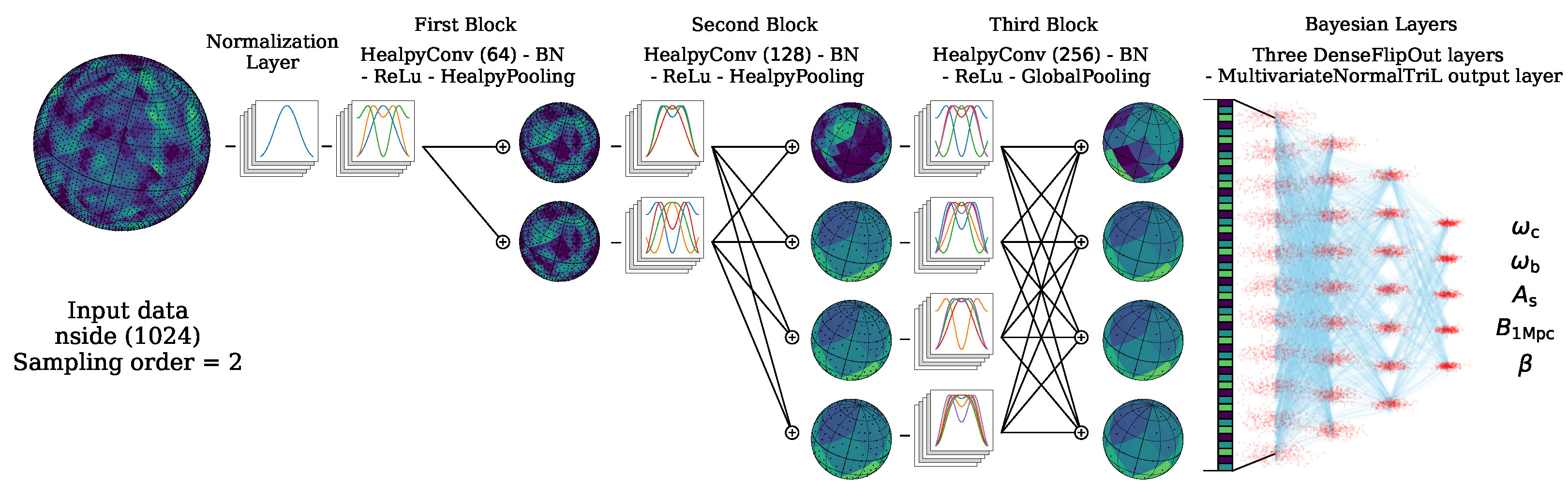
The network architecture was inspired by the DeepSphere global regression design [24] and implemented using TensorFlow with HealpyGCNN layers. It was designed to combine spherical convolutional feature extraction with Bayesian dense layers for probabilistic regression. The overall architecture consists of three main stages: normalization layer, hierarchical spherical convolution and pooling layers, and Bayesian dense layers for regression, as depicted in Figure 1.
The input consists of full-sky spherical maps at resolution nside = 1024; then, we create samples by dividing the complete spheres in patches based on HEALPix sampling of order = 2, which corresponds to a second-level subdivision of the HEALPix grid. This procedure effectively group pixels into larger, non-overlapping patches that preserve the topological structure of the sphere. We applied an input normalization layer (N) based on the mean and variance of the training dataset by iterating over all input maps. These statistics were stored and later used to initialize the Normalization layer (https://keras.io/api/layers/preprocessing_layers/numerical/normalization/ (accessed on 19 January 2026)) in Keras which standardizes the inputs. We employed a sequence of HealpyPseudoConv and HealpyPool layers. These layers exploit the hierarchical structure of the HEALPix pixelization. Each block contains a HealpyPseudoConv layer (GC) with p = 1 , meaning that the convolution considers only the immediate neighbors on the sphere, and an increasing number of feature maps ( F out = 64 , 128 , 256 ), a batch normalization layer (BN), and a ReLU activation. Between blocks, we introduced spherical pooling layers (HealpyPooling, P) with average reduction of the resolution, nside. As the network gets deeper, the number of feature maps ( F out ) increases from 64 to 128 to 256, while the spatial resolution decreases due to pooling. This is a standard and powerful design pattern, used in architectures such as AlexNet [49] or ResNet [50]. The outputs of the last spherical convolutional block are added using a global average pooling layer (AV). This reduces the feature maps to a compact vector representation that can be passed to fully connected layers. To incorporate predictive uncertainty, we employed three DenseFlipout layers [51] from TensorFlow Probability with 256, 128, and 64 units, each using a ReLU activation. The Bayesian treatment is achieved through variational inference where weights are modeled as distributions with a posterior approximated by the Flipout estimator. The final regression layer is a Bayesian multivariate distribution. Specifically, we used DenseFlipout (https://www.tensorflow.org/probability/api_docs/python/tfp/layers/DenseFlipout (accessed on 19 January 2026)) to output the parameters of a MultivariateNormalTriL (https://www.tensorflow.org/probability/api_docs/python/tfp/distributions/MultivariateNormalTriL (accessed on 19 January 2026)) distribution [52] of dimension five (corresponding to ω c , ω b , A s , B 1 M p c , and  β = log 10 ( τ ν / τ B ) ).

3.4. Training

The regression network was trained to predict the five cosmological parameters from simulated CMB maps using a probabilistic approach. The input shape was defined as ( 32 , N pix , 3 ) , where 32 corresponds to the mini-batch size (i.e., the number of training examples processed simultaneously); N pix denotes the number of padded pixels per map and the factor of three corresponds to the channels of the simulation. The model was compiled with the Adam optimizer, using a learning rate of 1 × 10 4 , and the negative log-likelihood ( NLL ) along with KL as the loss function. In addition, mean squared error (MSE), mean absolute error (MAE), and the coefficient of determination ( R 2 score) were monitored as complementary metrics. The  R 2 score was computed using the r2score scikit-learn (https://scikit-learn.org/stable/modules/generated/sklearn.metrics.r2_score.html (accessed on 19 January 2026)) implementation, which measures the proportion of variance in the true cosmological parameters that can be explained by the model predictions [53]. It is defined as
R 2 = 1 i ( y i y ^ i ) 2 i ( y i y ¯ ) 2 ,
where y i are the true parameter values, y ^ i are the corresponding predictions, and  y ¯ is the mean of the true values. A value of R 2 = 1 indicates perfect predictions, while values close to zero imply that the model performs similarly to using the mean of the data.
Regarding callbacks, three training callbacks were included: (1) EarlyStopping with a patience of 25 and automatic restoration of the best weights, (2) ModelCheckpoint for saving the optimal weights during training, and (3) ReduceLROnPlateau, which decreased the learning rate by a factor of 0.6 after five consecutive non-improving validation steps, with a floor of 10 6 . These strategies have been widely adopted in deep learning to prevent overfitting and to stabilize optimization in non-convex loss landscapes [54]. Training was performed for 300 epochs with a batch size of 32. The total number of trainable parameters is approximately 3.8 × 10 5 . The architecture combined Healpy-based convolutional layers for feature extraction with Bayesian dense layers for uncertainty-aware regression, resulting in an end-to-end model capable of mapping spherical CMB realizations to cosmological parameters.

3.5. Uncertainty Calibration

Uncertainties in deep neural networks tend to be under- or over-confident in their predictions. One way to diagnose the quality of uncertainty is through reliability plots [55]. Calibrating neural networks during training is not efficient in most cases because it affects the model’s performance. However, post hoc methods applied after training preserve the precision achieved during the training period [31]. We leverage post hoc calibration to improve the reliability of the uncertainty estimates. In the context of Bayesian regression, well-calibrated uncertainty estimates are essential for ensuring that predictive intervals reflect true empirical coverage. We employed the NetCal calibration framework (https://github.com/EFS-OpenSource/calibration-framework (accessed on 19 January 2026)), which has been extended to support probabilistic regression tasks. These techniques aim to adjust the predictive distribution outcomes such that the nominal coverage of predictive intervals aligns with their observed coverage. In fact, we implemented two post hoc calibration methods introduced in [48], the Variance Scaling and GPNormal. The VarianceScaling method applies a correction factor, α , to rescale the predictive variance σ cal 2 = α · σ pred 2 and re-calibrate the uncertainties. GPNormal, on the other hand, uses a Gaussian process to map the predictive mean and variance to calibrated uncertainty estimates, allowing for more flexible non-linear transformation of the uncertainty space [48].

4. Results

In this section we report the results obtained using two simulated datasets that differ in their scalar components: full and prim-vp. Both datasets were used to train and evaluate the same neural network model described previously, with the goal of predicting the five cosmological parameters listed in Table 1. To assess the model’s performance, we evaluated it on the respective validation and test sets and computed two key metrics—mean squared error (MSE) and mean absolute error (MAE)—along with the loss function described by Equation (1). Additionally, an external dataset was employed as a held-out test set. This dataset was never used during training or hyperparameter tuning and serves solely to evaluate the model’s generalization performance. Table 2 summarizes the evaluation results for both datasets.
We observe that the model reaches comparable training stability across both datasets. However, the full outperformed the prim-vp dataset across all three metrics. Since MSE penalizes larger errors more heavily, its lower value shows that the model was more effective at suppressing outlier predictions when trained with the full scalar input. These results demonstrate that the scalar input in the full dataset enhances the model’s capacity to learn the underlying mapping between CMB features and cosmological parameters, including the effects of primordial magnetic fields.
Table 3 reports the R 2 for each parameter in both experiments. Beyond the quantitative metrics, these results also highlight how the inclusion of the scalar contribution affects the network’s ability to disentangle the physical dependencies among parameters. The improvement observed in the full configuration, particularly for ω c and β , shows that scalar information provides complementary features that help the model to predict with better results. Baryon density and the magnetic field are the best-predicted parameters in both datasets with high precision, while the magnetic damping scale obtained the lowest value, especially in the prim-vp case, which lacks the scalar component. The strong R 2 achieved for B 1 Mpc in both datasets indicates that the network effectively captures the imprint of the magnetic field amplitude on the CMB spectra, despite the complex interplay between PMF-induced and standard cosmological signals. This result is encouraging, as it shows that machine learning methods can detect magnetic signatures even when trained on broad parameter priors.
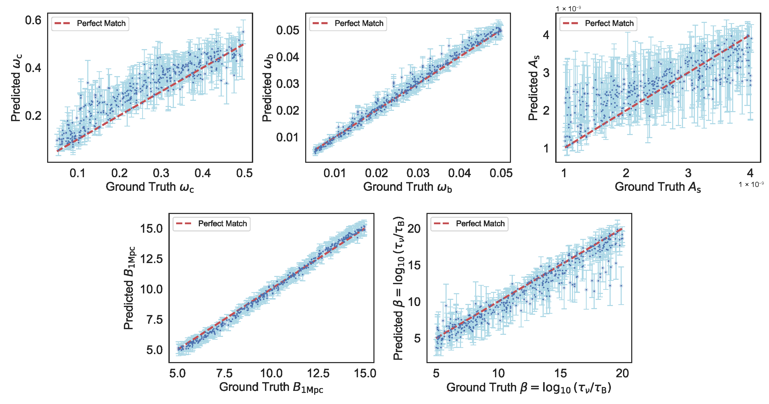
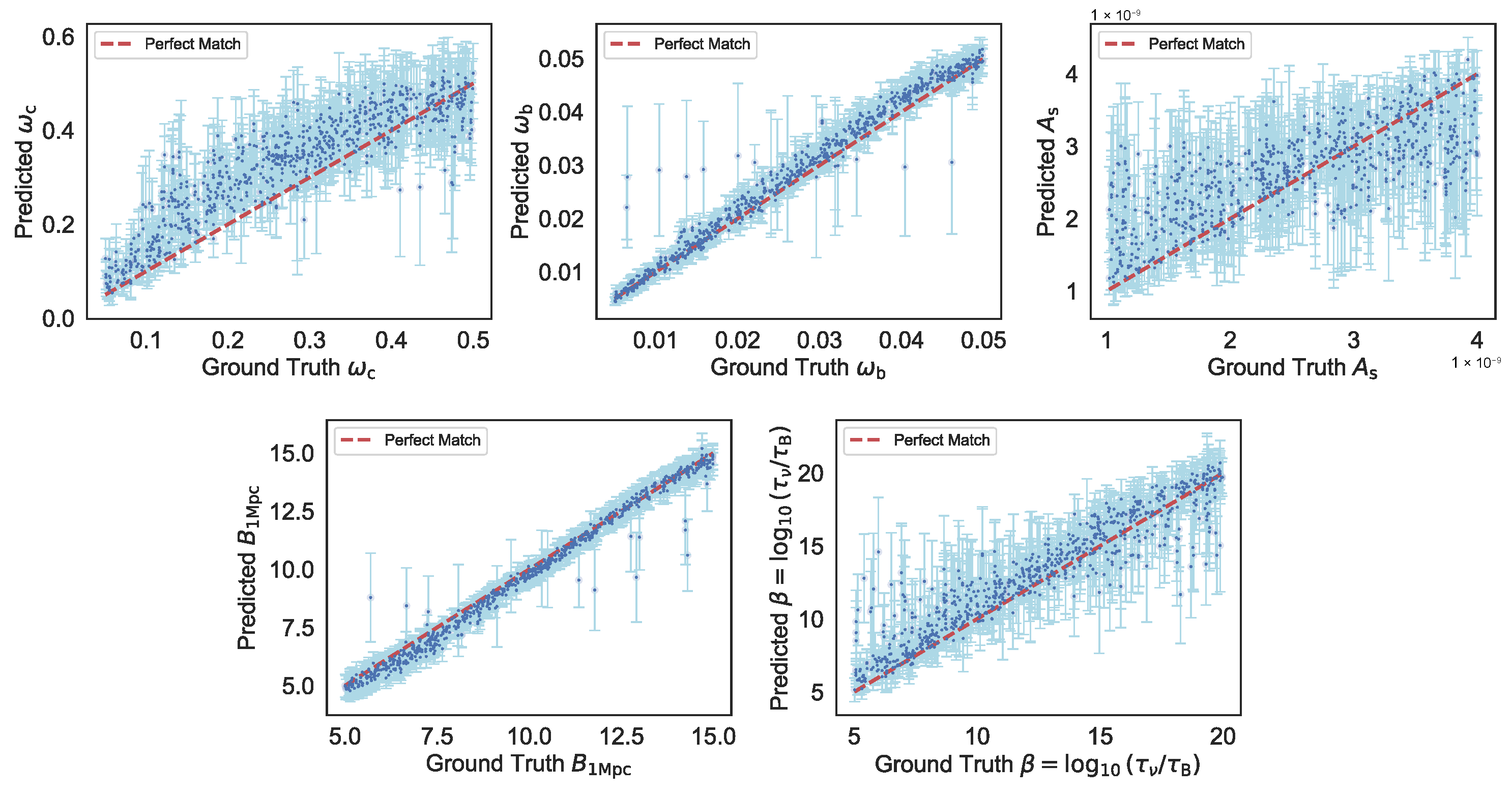
Figure 2 shows the predicted values versus the ground truth for each of the five parameters in the full dataset. The red dashed line represents the perfect match. Most predictions align well along this line, especially for B 1 Mpc and ω b , confirming the strong performance seen in the R 2 scores. It is also worth noting that the relatively moderate performance for A s and ω c reflects the inherent degeneracies between these parameters and others in the CMB, a well-known limitation in cosmological parameter estimation. Beyond the R 2 scores, the regression performance can also be assessed through the complementary metrics reported in Table 2, the mean squared error (MSE) and mean absolute error (MAE). The low values achieved by both metrics indicate that the model not only captures the global variance of the data (as reflected in the high R 2 ) but also maintains a small average deviation between predictions and ground truth values. This consistency across metrics and the consistency between the validation, test, and external sets supports the model’s ability to generalize over unseen data and reinforces the reliability of its predictions. Together, these results confirm that the proposed architecture achieves both precision and robustness in learning the nonlinear mapping between CMB features and cosmological parameters.
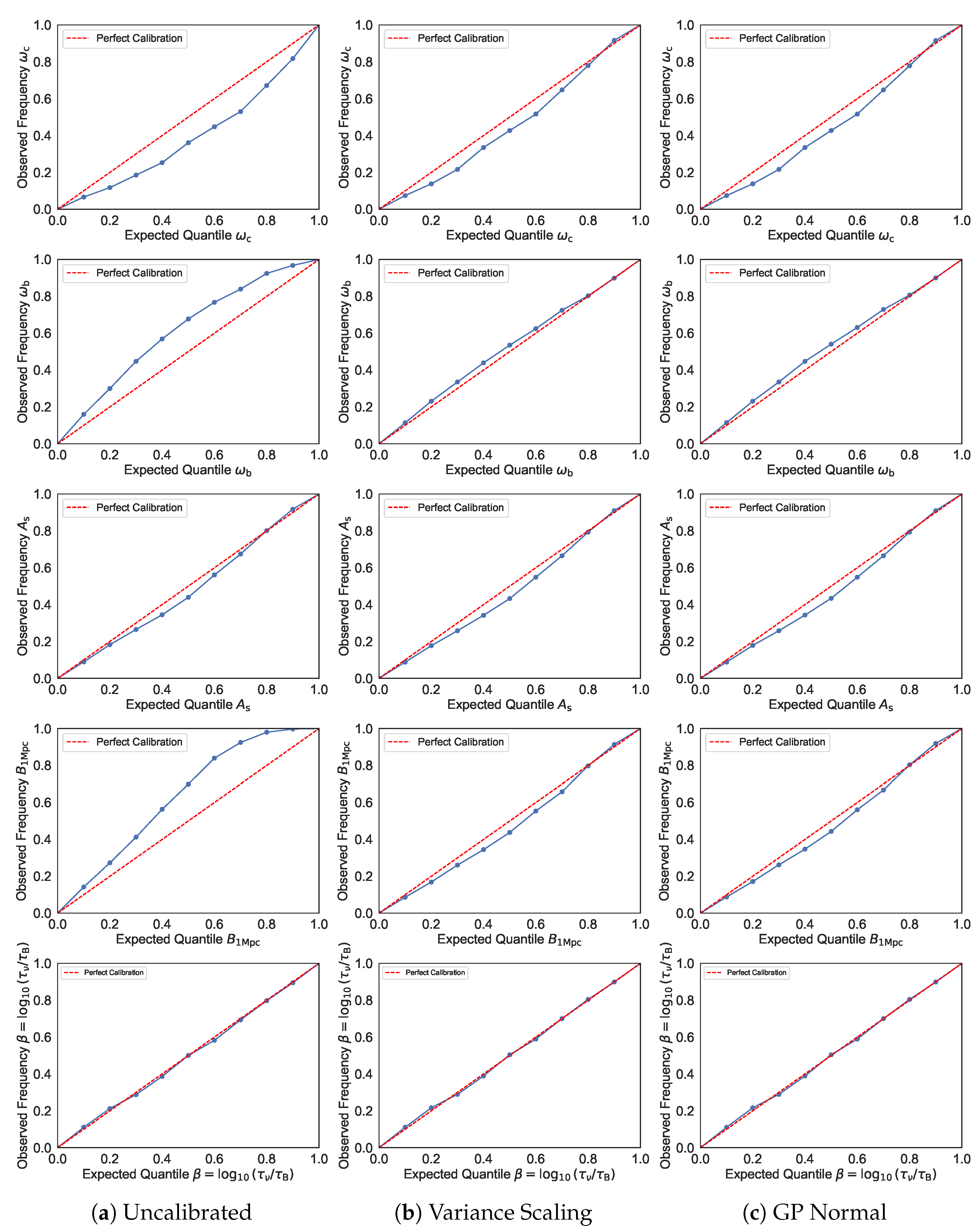
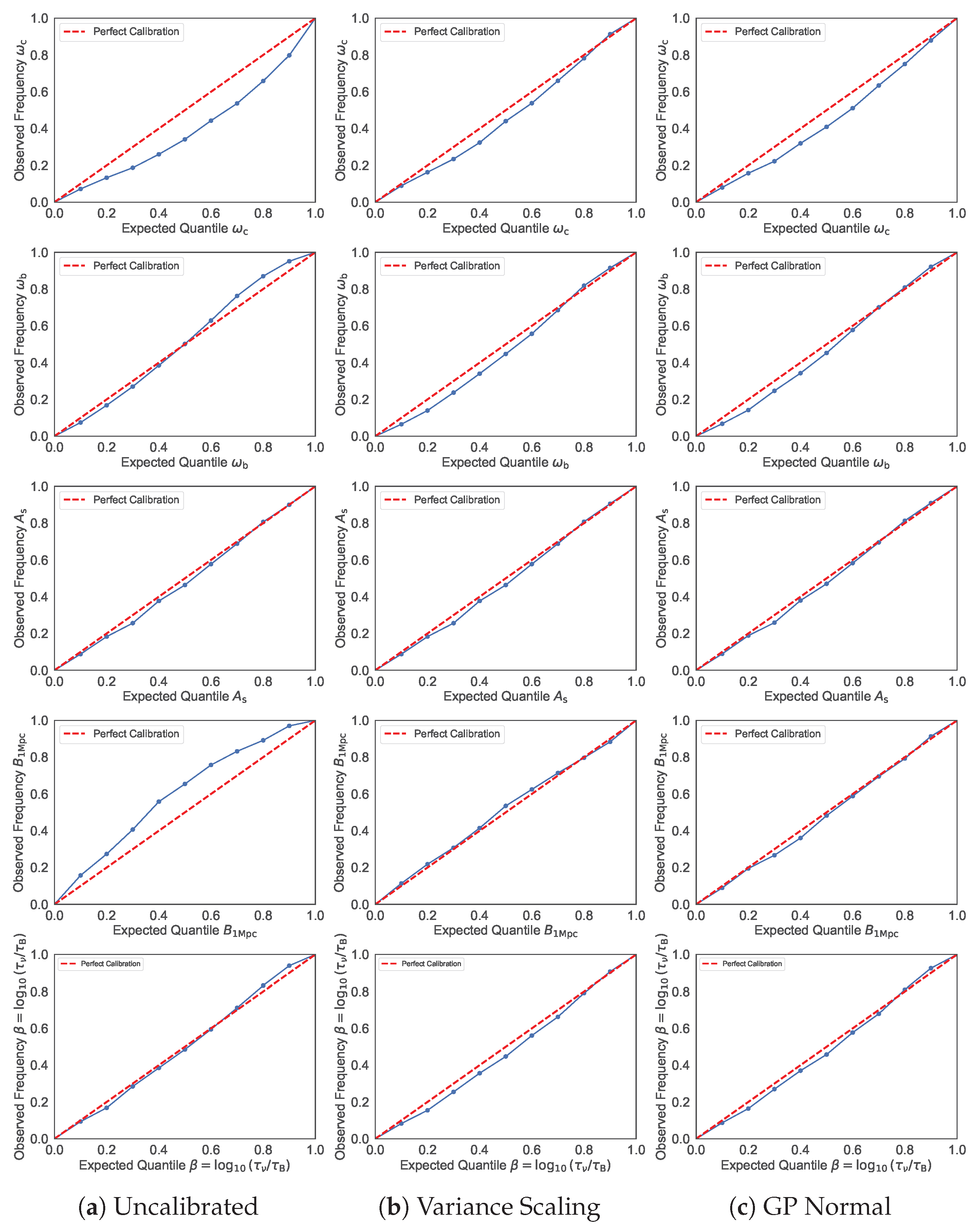
The error bars represent the predicted standard deviation of the output distribution. Parameters with lower R 2 tend to have larger uncertainty, indicating the model is also less confident when predictions are less accurate. Nevertheless, the resulting uncertainty estimates may still be uncalibrated due to the model misspecification or approximation errors [56]. In Figure 3 we display the reliability diagrams when we use VarianceScaling and GPNormal calibrations for the five output dimensions. Each plot compares the expected quantile against the observed frequency.
Regarding the uncalibrated curves (see Figure 3a), the parameters with the highest R 2 scores— ω b and B 1 Mpc —show clear overconfidence from 0.2 to 0.8 in the expected quantile. In  B 1 Mpc the overconfidence is more remarkable in quantile 0.6. The predicted confidence intervals are too narrow and capture fewer true values than expected; even when point predictions are highly accurate, the associated uncertainty estimates can still be miscalibrated. On the other hand, the parameters A s and β = log 10 ( τ ν / τ B ) , which have lower R 2 scores, show well-calibrated, even slightly under-confident behavior of A s in quantile 0.5, resulting in curves that lie above the diagonal. After applying post hoc calibration (see Figure 3b,c), both VarianceScaling and GPNormal improve the alignment between predicted confidence levels and empirical frequencies, thereby reporting reliable uncertainties for our results. After applying the calibration procedure, it is important to fine-tune the model incorporating the recalibration adjustments to ensure that these corrections are consistent with the learned representations. Otherwise, post hoc corrections may lead to a mismatch between the adjusted uncertainty estimates and the actual error distribution. This principle has been discussed in the recent literature, where integrating calibration directly into the training loop has been shown to improve both reliability and generalization [57].
Importantly, these calibration effects have direct implications for the physical interpretation of the inferred PMF constraints. In the uncalibrated case, the overconfident uncertainty estimates on B 1 Mpc would lead to artificially tight confidence intervals, potentially resulting in spurious detections or overly aggressive exclusions of PMF scenarios. After calibration, the posterior intervals broaden in regimes where the PMF signal is weak or degenerate with cosmic variance and instrumental noise, yielding conservative and statistically meaningful upper limits on B 1 Mpc . Conversely, when the PMF imprint on the CMB is informative, the calibrated uncertainties contract appropriately, allowing robust exclusion of specific PMF models and enabling principled model comparison. These features are particularly relevant for forthcoming CMB experiments such as the CORE [58] and LiteBIRD [59], where subtle PMF signatures coexist with complex systematics and potential simulation-to-data mismatches. In this context, calibrated uncertainties provide a safeguard against overinterpretation, ensuring that model selection and hypothesis testing are driven by genuine physical information rather than miscalibrated confidence estimates. As a result, the calibrated framework strengthens the robustness and credibility of PMF constraints derived from next-generation CMB observations.

5. Discussion

We discuss the main experimental and architectural challenges found during the implementation of the Bayesian graph neural network. The computational process was executed using two NVIDIA TESLA V100-SXM2 GPUs running on the Google Cloud Platform. The initial architecture suggested by the main DeepSphere paper [24]—i.e., N N = A V G C σ G C P σ B N G C —proved effective for predicting a single cosmological parameter. Here, G C denotes a graph convolutional layer implemented on the HEALPix sphere, σ is the activation function (ReLU), B N corresponds to batch normalization, P denotes pooling, and  A V represents a global average layer used to aggregate the node features into a single vector. The normalization layer showed instability and tended toward infinite values because of large outputs in the input data. After the data cleaning phase to remove these outliers, the normalization layer stabilized and assumed reliable values. Encouraged by the promising performance of the model when predicting a single cosmological parameter, we generated a new dataset to explore the joint prediction of two parameters by mixing various PMF components. Nevertheless, the original architecture was not scalable and failed to converge when trained to predict multiple parameters simultaneously. To address this issue, the architecture was modified by adding a similar block to the original structure, and the number of convolutional filters was increased. Regarding the pooling operation, experimenting with both Average and Maximum strategies revealed a performance dependency on the output size. The Max pooling yielded better results for predicting a single parameter, whereas AVG pooling provided superior performance for the simultaneous prediction of multiple cosmological parameters. Subsequent success with two parameters lead to the creation of datasets for three parameters and then four parameters. In this scenario, three dense layers were applied instead of two for better performance. We identified and selected the two best performing datasets, full and prim-vp, chosen based on preliminary results that showed the highest R 2 scores across the four parameters (see Table A1 of Appendix A) which were then used to generate the final datasets for the prediction of the cosmological parameters. The training was conducted using a batch size of 32 and a learning rate of 1 × 10 4 . The training time was on average 8 s per step for 108 steps per epoch, resulting in approximately 860 s per epoch. In contrast to the deterministic model, the probabilistic model exhibited superior training stability and did not require stabilization techniques such as ReduceLROnPlateau or EarlyStopping to avoid divergence. The final model has 382,868 parameters. We have published a subset of the dataset on Zenodo (https://doi.org/10.5281/zenodo.17400503 (accessed on 20 October 2025)) for public access and further use, and the scripts used in this analysis are publicly available in the following repository BSCNN (https://github.com/JavierOrjuela/Bayesian-SphericalCNN (accessed on 19 January 2026)).

6. Conclusions

In this work, we have introduced a novel Bayesian graph deep learning framework for estimating key cosmological parameters from simulated full-sky CMB maps, explicitly incorporating contributions from PMFs through their passive and vector modes. By extending the DeepSphere spherical convolutional neural network with Bayesian Neural Network layers, our approach simultaneously leverages the geometry of spherical data and provides rigorous uncertainty quantification. The main conclusions of our study can be summarized as follows:
(i)
High predictive accuracy through integration of physical characteristics. The proposed B-GNN model achieved R 2 scores close to 90 % for most of the five cosmological parameters considered: ω b , ω c , A s , B 1 Mpc , and  β = log 10 ( τ ν / τ B ) . Moreover, we reported a mean absolute error (MAE) of 0.151 and a mean squared error (MSE) of 0.052 on an independent test set, confirming its strong generalization. Furthermore, the uncertainty estimates provided by the BNN were excellently calibrated, as shown in Figure 3. We found that the inclusion of PMF-induced passive and vector modes was crucial for improving the model’s representational power. This is clearly reflected in the superior performance of the full dataset compared to prim-vp, demonstrating that embedding relevant physical information in the input enhances the accuracy and stability of the predictions.
(ii)
Reliable and calibrated uncertainty quantification. A central contribution of this work is the incorporation of predictive uncertainty estimates. Although the raw uncertainty outputs of the probabilistic model exhibited over-confidence, applying post hoc calibration methods such as VarianceScaling and GPNormal effectively corrected this behavior. The resulting calibrated confidence intervals accurately matched the empirical error distribution, thereby increasing the interpretability and reliability of the model’s predictions. This is particularly important in cosmology, where well-calibrated uncertainties are essential for meaningful parameter inference.
(iii)
Strong generalization and architectural robustness. The model showed stable performance across independent validation datasets, confirming its ability to generalize beyond the training distribution. This robustness is the result of a carefully designed training strategy, including regularization, optimal learning rate scheduling, and dropout. Importantly, unlike the deterministic baseline, the Bayesian model maintained stability without requiring additional early stopping or learning-rate reduction techniques, further supporting its suitability for real data applications.
(iv)
Advancement of cosmological parameter inference with Bayesian deep learning. Compared to traditional parameter estimation techniques, this framework integrates a spherical CNN architecture with Bayesian inference principles, enabling both accurate point predictions and principled uncertainty estimation within a single model. Once trained, the network provides near-instantaneous parameter estimates, bypassing the computational cost of traditional MCMC methods.
(v)
The approach presented in this paper is best viewed as complementary to traditional methods. In fact, hybrid schemes using Bayesian Neural Networks to accelerate MCMC sampling preserve Bayesian rigor while dramatically improving efficiency [23]. However, recent proposals might be advantageous. For example, some neural-network-based methods enable near-optimal map-level inference while naturally incorporating masking, inhomogeneous noise, and non-Gaussianities. Examples include neural implementations of Wiener filtering that match conjugate-gradient accuracy at a fraction of the cost and improve upon pseudo-correlators estimators for complex sky masks [60], as well as spherical CNNs that constrain primordial non-Gaussianity directly from maps, avoiding bispectrum-based information loss [61]. Simulation-based inference further bypasses explicit likelihood assumptions, allowing systematics and nonlinearities to be propagated consistently into posterior constraints, yielding tighter bounds than power-spectrum-only analyses in weak lensing [62] and 21 cm cosmology [63]. The benefits are especially pronounced for non-Gaussian, high-dimensional signals such as 21 cm tomography, where map-level neural inference exploits information beyond two-point statistics [64,65]. Bayesian Neural Networks and normalizing flows further enable calibrated uncertainties and fast likelihood-free inference at a fraction of the computational cost of conventional pipelines [66].
(vi)
Outlook and implications for future applications. Our results indicate that a well-calibrated Bayesian Neural Network can robustly infer cosmological parameters from complex, high-dimensional CMB data that include subtle physical effects such as primordial magnetism. This framework offers a flexible and powerful alternative to conventional inference pipelines, providing not only point estimates but also interpretable uncertainty information. These characteristics make it a promising tool for future analyses for the next generation of CMB experiments, such as the PICO [67], LiteBIRD [59], and CORE [58]. These missions will deliver ultra-deep, high-resolution polarization maps where the PMF’s B-mode signal will be a critical and computationally challenging component to isolate. Our work establishes a foundation for using advanced machine learning to harness this data, offering a powerful and complementary tool to traditional methods for probing fundamental physics in the early Universe.
In summary, this study demonstrates that probabilistic deep learning methods, when carefully designed and systematically calibrated, can significantly enhance the precision and reliability of cosmological parameter estimation from CMB data. The integration of physical information, spherical geometry, and Bayesian inference principles offers a new and powerful pathway to tackle open questions in cosmology and to explore beyond-standard physics.

Author Contributions

Conceptualization, H.J.H.; Methodology, H.J.H. and J.E.G.-F.; Software, H.J.H. and J.A.P.C.; Validation, J.A.P.C.; Formal Analysis, J.A.P.C.; Investigation, all authors have contributed equally; Resources, R.A.H.; Data Curation, J.E.G.-F.; Writing—Original Draft Preparation, all authors have contributed equally; Writing—Review and Editing, J.A.P.C. and R.A.H.; Visualization, J.A.P.C. and R.A.H.; Supervision, H.J.H. and J.E.G.-F. All authors have read and agreed to the published version of the manuscript.

Funding

This research was supported by the Google Cloud Research Credits program with the award GCP19980904.

Data Availability Statement

The original data presented in the study are openly available in https://zenodo.org/records/17400503 (accessed on 20 October 2025).

Conflicts of Interest

The authors declare no conflicts of interest.

Appendix A

Appendix A.1. Selection of Best Results

We chose these two dataset full and prim-vp due to preliminary results with a deterministic model and four cosmological predictable parameters:
Table A1. Coefficient of determination ( R 2 ) for the prediction of four cosmological parameters across all simulated datasets. Each column corresponds to one target parameter: the cold dark matter density ( ω c ), the scalar amplitude ( A s ), the magnetic field strength smoothed at 1 Mpc ( B 1 Mpc ), and magnetic damping scale β = log 10 ( τ ν / τ B ) . The first column reports the mean R 2 over all parameters.
Datasets R 2 ω c A s B 1 Mpc β = log 10 ( τ ν / τ B )
full0.8940.9110.7580.9930.913
prim-vp0.8800.8910.8420.9230.863
svp0.8600.8760.6600.9920.912
vp0.8000.9590.2580.9960.985
prim-sv0.7830.9200.9560.9770.281
prim-v0.7750.9510.9800.9900.179
sv0.5410.9550.0690.9920.148
prim-s0.2290.3510.888−0.119−0.206
sp0.209−0.040−0.1020.7250.251
prim-sp0.054−0.0110.0430.1810.005
These results helped us to determine the two best datasets for modifying the dense layers with Bayesian layers, thereby obtaining more reliable results thanks to the implementation of uncertainty quantification. The deterministic model achieved better results of R 2 in full and prim-vp, achieving 0.894 and 0.88 , respectively. In contrast, the remaining datasets show notably lower R 2 scores, which suggests that the absence of certain perturbation modes limits the model’s ability to recover the full parameter space. This pattern highlights the importance of including multiple mode contributions in the simulated CMB maps. In particular, datasets that include the vectorial and passive (vp) modes consistently yield the highest correlations, indicating that these components encode essential physical information that improves the model’s capacity to recover the cosmological parameters. After selecting the two best datasets and configuring the probabilistic model as B-GNN, we generated the corresponding datasets with five cosmological parameters to be predicted and applied a data-cleaning procedure.

Appendix A.2. Data Cleaning

The data cleaning process corresponds to dropping the outliers from the dataset. These outliers have huge values compared with the central tendency of the CMB maps. We present the comparison of the dataset before and after the cleaning process.
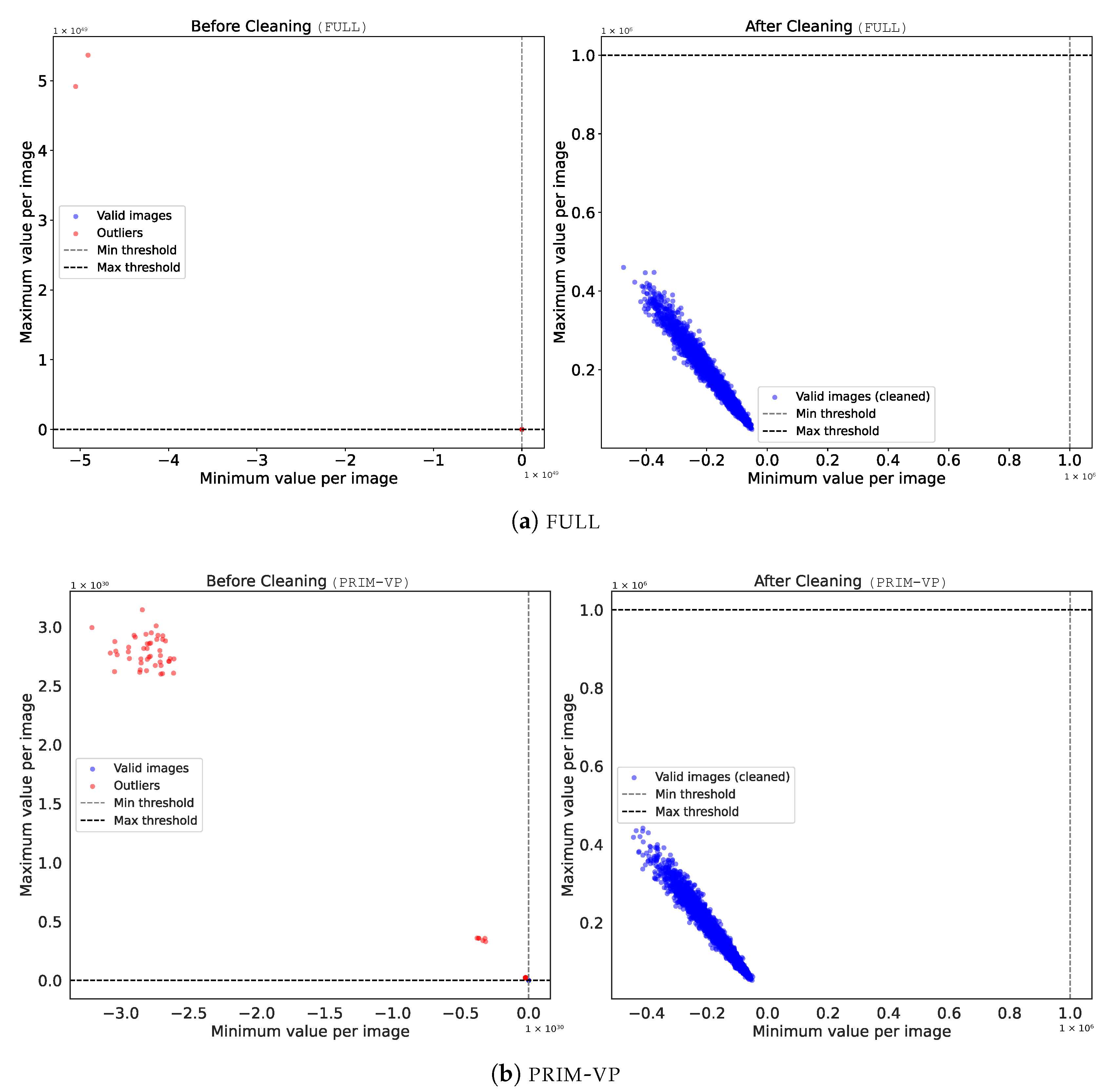
The scatter plots in Figure A1 correspond to the data cleaning process in the full and prim-vp dataset, illustrating the distribution of the minimum and maximum pixel values per image before and after applying the outlier cleaning procedure. The data cleaning procedure removes extreme outliers present in the simulation of the CMB maps. These anomalies were clearly visible because of the huge difference in scale comparing the left panel (before cleaning) and the right panel (after cleaning). The left panels present a scale of 1 × 10 49 while the right panels present a scale of 1 × 10 6 . The presence of these outliers far away from the main points affected the normalization step, driving the feature scaling to divergent values and destabilizing the training process. After removal, both datasets showed consistent range, as observed in the right panels. The cleaning steps were crucial to guarantee numerical stability and reliable model calibration.
Figure A1. Scatter plots of the minimum vs. maximum pixel values per image before and after outlier removal. The left panel shows the raw data, where extreme outliers reach values up to 1 × 10 30 . Panels (a) correspond to the full dataset, and panels (b) to the prim-vp dataset. The left panels show the distribution of the minimum and maximum pixel values per image before cleaning. The right panel displays the cleaned dataset after applying the thresholds with value 1 × 10 6 . Dashed lines indicate the minimum and maximum thresholds used for cleaning.
Universe 12 00034 g0a1

Appendix A.3. Contribution of Relevant Magnetic Modes

Primordial magnetic fields (PMFs) affect the Cosmic Microwave Background (CMB) through their contribution to the energy–momentum tensor and the Lorentz force acting on the baryon–photon plasma prior to recombination. In the magnetohydrodynamic (MHD) limit, valid in the highly conducting early Universe, the comoving magnetic field evolves as B ( x , τ ) = B ( x , τ 0 ) / a 2 ( τ ) and electric fields are negligible. The stress–energy tensor associated with the PMF is quadratic in the field amplitude and can be written as [43]
T B 0 0 ( x , τ ) = 1 8 π a 4 B 2 ( x ) , T B j i ( x , τ ) = 1 4 π a 4 1 2 B 2 ( x ) δ j i B i ( x ) B j ( x ) ,
which defines an effective magnetic energy density contrast Δ B and an anisotropic stress tensor Π B j i . The anisotropic stress is the key quantity sourcing metric perturbations and can be decomposed into scalar, vector, and tensor components. As a result, PMFs generate all types of cosmological perturbation modes, including vorticity and gravitational waves, even in the absence of primordial inflationary tensor modes. The magnetic field is modeled as a statistically isotropic, Gaussian random field with power spectrum  P B ( k ) k n B , with n B being the magnetic spectral index. The quadratic nature of the magnetic stress–energy tensor implies that PMF-induced CMB anisotropies are intrinsically non-Gaussian; however, at the level of two-point statistics, their effect is fully captured by the power spectra of Δ B and Π B . Depending on the epoch of magnetic field generation relative to neutrino decoupling, two classes of modes arise: passive modes, sourced before neutrino decoupling and growing logarithmically until compensation sets in, and compensated modes, continuously sourced afterward with neutrino anisotropic stress balancing the magnetic contribution.
In practice, the dominant observational signature of PMFs arises from the compensated vector modes, which survive Silk damping and generate significant B-mode polarization at small angular scales. The total theoretical CMB power spectra can therefore be written as a linear sum (Equation (2)), where the magnetic contributions are treated as statistically independent from the standard inflationary perturbations. This decomposition forms the theoretical basis for incorporating PMFs into Boltzmann solvers such as CAMB and for predicting their imprint on CMB temperature and polarization anisotropies.
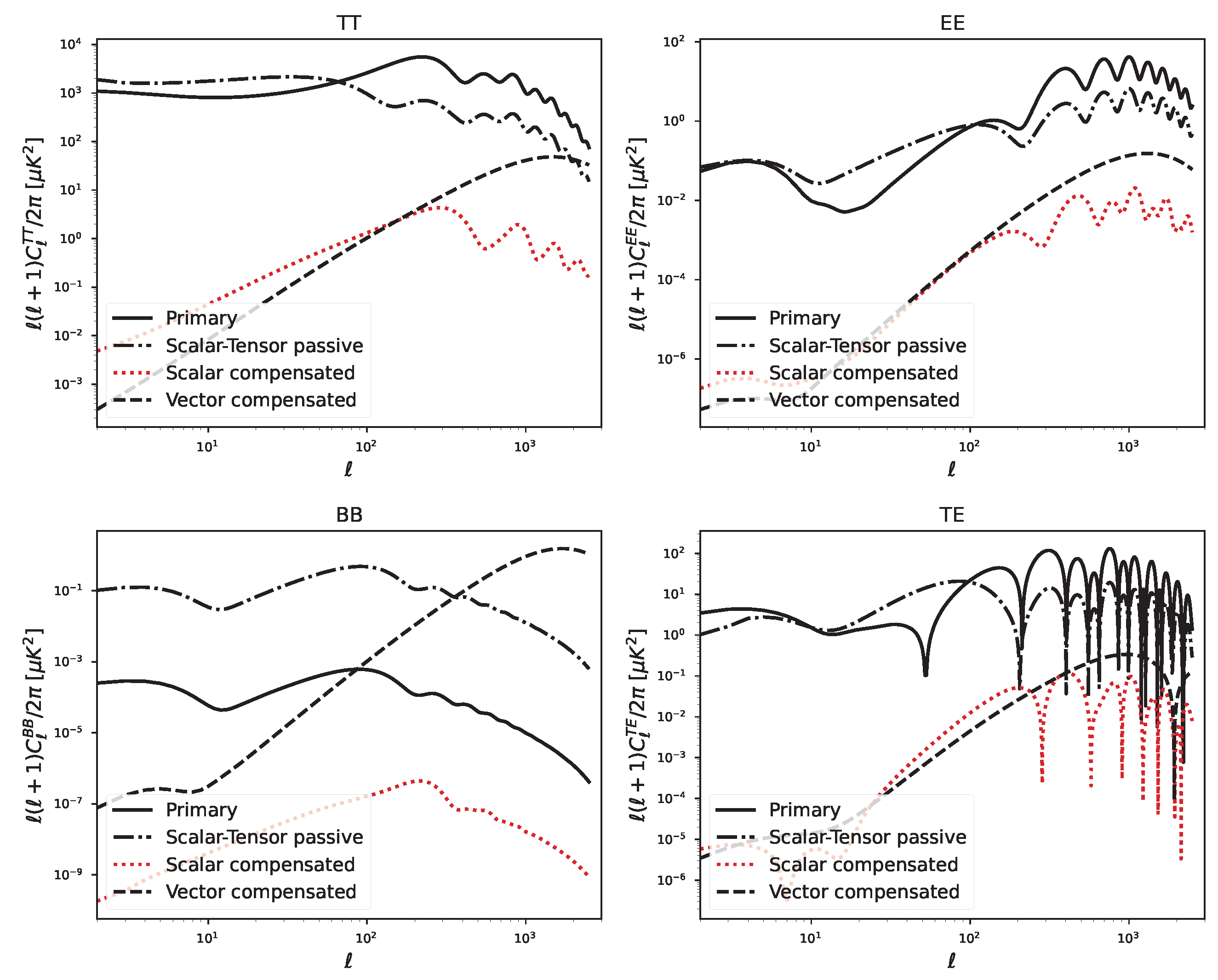
We show that the individual contributions to the CMB temperature and polarization power spectra generated by PMFs follow the decomposition mode described in [22]. The spectra are computed using a modified pipeline based on CAMB [42,43] and displayed in the standard form ( + 1 ) C / 2 π . Figure A2 contains four panels (TT, EE, BB, and TE), each showing the FULL CMB spectra separated into the non-magnetic component (labeled primary, following the notation in [22]), the scalar–tensor passive magnetic mode, the scalar compensated magnetic mode, and the vector compensated magnetic mode.
Figure A2. Individual contributions to the CMB temperature and polarization power spectra generated by primordial magnetic fields (PMFs) with cosmological parameters set as B 1 Mpc = 5 nG, n B = 2.9 , β = log 10 ( τ ν / τ B ) = 17 , ω b = 0.0226 , ω c = 0.112 , A s = 2.1 × 10 9 , and n s = 0.96 .
Universe 12 00034 g0a2
In TT and EE, the dominant magnetic signal at low arises from the passive mode, sourced by tensor perturbations prior to neutrino decoupling, while the scalar- and vector-compensated modes contribute subdominant, smooth corrections, with the vector mode becoming more relevant only at high multipoles. The BB spectrum exhibits the clearest magnetic signature: passive tensor perturbations generate power on large scales, whereas the compensated vector mode dominates on small scales, producing the characteristic steep rise at high that is well documented in Planck results, see, e.g., the constrains on PMFs (2015) [46]. These vector modes survive Silk damping down to very small angular scales and are therefore a major source of constraining power for PMFs, especially through the velocity field sourced by the Lorentz force. Consistent with previous analyses (e.g., [22]; [20]), this small-scale vector-induced signal represents one of the most informative features in the magnetic contribution to the CMB. Together, these components highlight the scale dependence and physical origin of the magnetic modes included in the FULL dataset used in our analysis.

Appendix A.4. Supplementary PRIM-VP Results

While the main purpose of this paper focused on full results, an analysis of prim-vp results is presented. We report the R 2 of the five cosmological parameters.
Figure A3. Predicted versus ground truth true values for the five cosmological parameters using the prim-vp. Each subplot corresponds to one parameter, with the black dashed line representing the ideal prediction. Shaded bars denote one standard deviation.
Universe 12 00034 g0a3
Among the parameters, ω b and B 1 , Mpc display the most accurate constrained predictions. In contrast, A s and β show slightly higher scatter and wider uncertainty ranges; these parameters are more degenerated in the input features. Nonetheless, the overall alignment between predicted and true values confirms that the probabilistic model effectively captures both the mean trends and the associated uncertainties of the cosmological parameters. The large standard deviation for certain points out of the diagonal, particularly pronounced in Ω b and β = log 10 ( τ ν / τ B ) , can be attributed to a combination of data imbalance, physical degeneracies, and intrinsic limitations of the learning process, which results in a wide predictive posterior distribution from the B-GNN due to less training samples. First, the training set contains fewer samples in the extreme regions of the parameter space, particularly for combinations of very low magnetic field amplitude B 1 , Mpc and very high β = log 10 ( τ ν / τ B ) . As a consequence, the neural network receives limited exposure to these regions during training, leading to poor generalization. Predictions in such sparsely populated corners are therefore more susceptible to extrapolation errors, which naturally manifest as points far from the diagonal. Second, in regimes where the PMF amplitude is low, the PMF-induced signal becomes subdominant with respect to cosmic variance and instrumental noise. In this limit, different realizations of the sky can produce maps that are statistically very similar to the Λ CDM case, even when the underlying PMF parameters differ. This introduces an intrinsic degeneracy in the mapping between observables and parameters: the network may confuse a genuinely low-B realization with a moderate-B realization affected by an unfavorable noise or cosmic variance fluctuation. As a result, a small number of samples can be assigned predictions that lie far from their true values. Third, these off-diagonal points reflect a fundamental ambiguity rather than a pure modeling failure. When the signal-to-noise ratio is low, the posterior distribution of the parameters becomes broad and potentially multimodal. Since the network is trained to produce point estimates, it is forced to commit to a single prediction, which may deviate from the ground truth even though it remains statistically plausible. On the other hand, these results contrast with those obtained using the FULL dataset, where the number of outliers is substantially reduced. The FULL dataset provides a more uniform coverage of the parameter space, allowing the model to better learn the relevant correlations and break degeneracies. The improved convergence and reduced scatter around the diagonal therefore reflect the additional information content and improved sampling rather than a change in the network architecture itself.
Figure A4. Uncertainty calibration curves (reliability diagrams) for each predicted parameter using the prim-vp dataset. The plots compare predicted Expected quantile (x-axis) with the observed frequencies (y-axis). Perfect calibration corresponds to the dashed red diagonal. (a) Uncalibrated model outputs, (b) post hoc calibration using VarianceScaling. (c) Post hoc calibration using GPNormal.
Universe 12 00034 g0a4
Also, we assessed the quality of the parameter uncertainties and overall calibration of the results. Figure A4 displays reliability diagrams comparing the observed versus expected frequencies of the predicted uncertainty quantiles, allowing assessment of the probabilistic calibration of the model. The red dashed line represents perfect calibration, where predicted confidence intervals exactly match the empirical coverage. The model for B 1 M p c and Ω c parameters, in Figure A4a, are over-confident and under-confident, respectively. On the other parameters there is a favorable agreement between the predicted and the observed confidence levels. To reduce the miscalibration, we applied VarianceScaling (Figure A4b) and GPNormal (Figure A4c), reflecting an improved alignment between predicted and observed probabilities. This behavior demonstrates that the post hoc calibration procedures corrected the mismatch between nominal and empirical coverage, leading to well-calibrated predictive distributions.

References

  1. Hu, W. Lecture Notes on CMB Theory: From Nucleosynthesis to Recombination. arXiv 2008, arXiv:0802.3688. [Google Scholar] [CrossRef] [Scilit]
  2. Dodelson, S.; Schmidt, F. Modern Cosmology; Academic Press: Cambridge, MA, USA, 2020. [Google Scholar] [CrossRef] [Scilit]
  3. Simpson, G.; Bolejko, K.; Walters, S. Beyond ΛCDM: How the Hubble tension challenges early Universe physics. Class. Quantum Gravity 2025, 42, 143001. [Google Scholar] [CrossRef] [Scilit]
  4. Jia, X.D.; Hu, J.P.; Gao, D.H.; Yi, S.X.; Wang, F.Y. The Hubble Tension resolved by the DESI Baryon Acoustic Oscillations Measurements. arXiv 2025, arXiv:2509.17454. [Google Scholar] [CrossRef] [Scilit]
  5. Hu, J.P.; Wang, F.Y. Hubble Tension: The Evidence of New Physics. Universe 2023, 9, 94. [Google Scholar] [CrossRef] [Scilit]
  6. Shiraishi, M. Polarization bispectrum for measuring primordial magnetic fields. J. Cosmol. Astropart. Phys. 2013, 2013, 006. [Google Scholar] [CrossRef] [Scilit]
  7. Shiraishi, M. Parity violation of primordial magnetic fields in the CMB bispectrum. J. Cosmol. Astropart. Phys. 2012, 2012, 015. [Google Scholar] [CrossRef] [Scilit]
  8. Rashkovetskyi, M.; Muñoz, J.B.; Eisenstein, D.J.; Dvorkin, C. Small-scale clumping at recombination and the Hubble tension. Phys. Rev. D 2021, 104, 103517. [Google Scholar] [CrossRef] [Scilit]
  9. Jedamzik, K.; Abel, T.; Ali-Haïmoud, Y. Cosmic recombination in the presence of primordial magnetic fields. J. Cosmol. Astropart. Phys. 2025, 2025, 012. [Google Scholar] [CrossRef] [Scilit]
  10. Schiff, J.; Venumadhav, T. Primordial magnetic fields and modified recombination histories. arXiv 2025, arXiv:2506.16517. [Google Scholar] [CrossRef] [Scilit]
  11. Widrow, L.M. Origin of galactic and extragalactic magnetic fields. Rev. Mod. Phys. 2002, 74, 775–823. [Google Scholar] [CrossRef] [Scilit]
  12. Neronov, A.; Vovk, I. Evidence for Strong Extragalactic Magnetic Fields from Fermi Observations of TeV Blazars. Science 2010, 328, 73. [Google Scholar] [CrossRef] [Scilit]
  13. Widrow, L.M.; Ryu, D.; Schleicher, D.R.G.; Subramanian, K.; Tsagas, C.G.; Treumann, R.A. The First Magnetic Fields. Space Sci. Rev. 2012, 166, 37–70. [Google Scholar] [CrossRef] [Scilit]
  14. Durrer, R.; Neronov, A. Cosmological magnetic fields: Their generation, evolution and observation. Astron. Astrophys. Rev. 2013, 21, 62. [Google Scholar] [CrossRef] [Scilit]
  15. Hortúa, H.J. Cosmological Features of Primordial Magnetic Fields. arXiv 2019, arXiv:1903.04419. [Google Scholar] [CrossRef] [Scilit]
  16. Kandus, A.; Kunze, K.E.; Tsagas, C.G. Primordial magnetogenesis. Phys. Rep. 2011, 505, 1–58. [Google Scholar] [CrossRef] [Scilit]
  17. Tsagas, C.G. Causality, initial conditions, and inflationary magnetogenesis. Phys. Rev. D 2016, 93, 103529. [Google Scholar] [CrossRef] [Scilit]
  18. Pogosian, L.; Vachaspati, T.; Yadav, A. Primordial magnetism in CMB B modes. Can. J. Phys. 2013, 91, 451–454. [Google Scholar] [CrossRef] [Scilit]
  19. Hortúa, H.J.; Castañeda, L. Reduced bispectrum seeded by helical primordial magnetic fields. J. Cosmol. Astropart. Phys. 2017, 2017, 020. [Google Scholar] [CrossRef] [Scilit]
  20. Pogosian, L.; Yadav, A.P.S.; Ng, Y.F.; Vachaspati, T. Primordial magnetism in the CMB: Exact treatment of Faraday rotation and WMAP7 bounds. Phys. Rev. D 2011, 84, 043530. [Google Scholar] [CrossRef] [Scilit]
  21. Sutton, D.R.; Feng, C.; Reichardt, C.L. Current and Future Constraints on Primordial Magnetic Fields. Astrophys. J. 2017, 846, 164. [Google Scholar] [CrossRef] [Scilit]
  22. Zucca, A.; Li, Y.; Pogosian, L. Constraints on primordial magnetic fields from Planck data combined with the South Pole Telescope CMB B-mode polarization measurements. Phys. Rev. D 2017, 95, 063506. [Google Scholar] [CrossRef] [Scilit]
  23. Hortua, H.J.; Volpi, R.; Marinelli, D.; Malago, L. Accelerating MCMC algorithms through Bayesian Deep Networks. arXiv 2020, arXiv:2011.14276. [Google Scholar] [CrossRef] [Scilit]
  24. Perraudin, N.; Defferrard, M.; Kacprzak, T.; Sgier, R. DeepSphere: Efficient spherical convolutional neural network with HEALPix sampling for cosmological applications. Astron. Comput. 2019, 27, 130. [Google Scholar] [CrossRef] [Scilit]
  25. Defferrard, M.; Milani, M.; Gusset, F.; Perraudin, N. DeepSphere: A graph-based spherical CNN. arXiv 2020, arXiv:2012.15000. [Google Scholar]
  26. Defferrard, M.; Perraudin, N.; Kacprzak, T.; Sgier, R. DeepSphere: Towards an Equivariant Graph-Based Spherical CNN. In Proceedings of the ICLR 2019 Workshop on Representation Learning on Graphs and Manifolds, New Orleans, LA, USA, 6 May 2019; Available online: https://rlgm.github.io/papers/71.pdf (accessed on 20 October 2025).
  27. Górski, K.M.; Hivon, E.; Banday, A.J.; Wandelt, B.D.; Hansen, F.K.; Reinecke, M.; Bartelmann, M. HEALPix: A Framework for High-Resolution Discretization and Fast Analysis of Data Distributed on the Sphere. Astrophys. J. 2005, 622, 759–771. [Google Scholar] [CrossRef] [Scilit]
  28. Krachmalnicoff, N.; Tomasi, M. Convolutional neural networks on the HEALPix sphere: A pixel-based algorithm and its application to CMB data analysis. Astron. Astrophys. 2019, 628, A129. [Google Scholar] [CrossRef] [Scilit]
  29. Gal, Y.; Ghahramani, Z. Dropout as a Bayesian Approximation: Representing Model Uncertainty in Deep Learning. In Proceedings of the 33rd International Conference on Machine Learning, New York, NY, USA, 20–22 June 2016; Volume 48, pp. 1050–1059. [Google Scholar]
  30. Dvorkin, C.; Mishra-Sharma, S.; Nord, B.; Villar, V.A.; Avestruz, C.; Bechtol, K.; Ćiprijanović, A.; Connolly, A.J.; Garrison, L.H.; Narayan, G.; et al. Machine Learning and Cosmology. arXiv 2022, arXiv:2203.08056. [Google Scholar] [CrossRef] [Scilit]
  31. Hortúa, H.J.; Volpi, R.; Marinelli, D.; Malagò, L. Parameter estimation for the cosmic microwave background with Bayesian neural networks. Phys. Rev. D 2020, 102, 103509. [Google Scholar] [CrossRef] [Scilit]
  32. García-Farieta, J.E.; Hortúa, H.J.; Kitaura, F.S. Bayesian deep learning for cosmic volumes with modified gravity. Astron. Astrophys. 2024, 684, A100. [Google Scholar] [CrossRef] [Scilit]
  33. Blundell, C.; Cornebise, J.; Kavukcuoglu, K.; Wierstra, D. Weight Uncertainty in Neural Network. In Proceedings of the 32nd International Conference on Machine Learning, Lille, France, 7–9 July 2015; Volume 37, pp. 1613–1622. [Google Scholar]
  34. Farsian, F.; Marulli, F.; Moscardini, L.; Giocoli, C. New Applications of Graph Neural Networks in Cosmology. In Machine Learning for Astrophysics; Springer: Cham, Switzerland, 2023; Volume 60, pp. 35–38. [Google Scholar] [CrossRef] [Scilit]
  35. Corso, G.; Stark, H.; Jegelka, S.; Jaakkola, T.; Barzilay, R. Graph neural networks. Nat. Rev. Methods Prim. 2024, 4, 17. [Google Scholar] [CrossRef] [Scilit]
  36. Bessadok, A.; Mahjoub, M.A.; Rekik, I. Graph Neural Networks in Network Neuroscience. IEEE Trans. Pattern Anal. Mach. Intell. 2023, 45, 5833–5848. [Google Scholar] [CrossRef] [Scilit]
  37. Zhang, S.; Tong, H.; Xu, J.; Maciejewski, R. Graph convolutional networks: A comprehensive review. Comput. Soc. Netw. 2019, 6, 11. [Google Scholar] [CrossRef] [Scilit]
  38. Xu, X.; Zhao, X.; Wei, M.; Li, Z. A comprehensive review of graph convolutional networks: Approaches and applications. Electron. Res. Arch. 2023, 31, 4185–4215. [Google Scholar] [CrossRef] [Scilit]
  39. Bronstein, M.M.; Bruna, J.; Cohen, T.; Veličković, P. Geometric Deep Learning: Grids, Groups, Graphs, Geodesics, and Gauges. arXiv 2021, arXiv:2104.13478. [Google Scholar] [CrossRef] [Scilit]
  40. Valentin Jospin, L.; Buntine, W.; Boussaid, F.; Laga, H.; Bennamoun, M. Hands-on Bayesian Neural Networks—A Tutorial for Deep Learning Users. arXiv 2020, arXiv:2007.06823. [Google Scholar] [CrossRef] [Scilit]
  41. Magris, M.; Iosifidis, A. Bayesian learning for neural networks: An algorithmic survey. Artif. Intell. Rev. 2023, 56, 11773–11823. [Google Scholar] [CrossRef] [Scilit]
  42. Lewis, A.; Challinor, A.; Lasenby, A. Efficient Computation of Cosmic Microwave Background Anisotropies in Closed Friedmann-Robertson-Walker Models. Astrophys. J. 2000, 538, 473–476. [Google Scholar] [CrossRef] [Scilit]
  43. Shaw, J.R.; Lewis, A. Massive neutrinos and magnetic fields in the early universe. Phys. Rev. D 2010, 81, 043517. [Google Scholar] [CrossRef] [Scilit]
  44. Mandal, S.; Sehgal, N.; Namikawa, T. Finding evidence for inflation and the origin of galactic magnetic fields with CMB surveys. Phys. Rev. D 2022, 105, 063537. [Google Scholar] [CrossRef] [Scilit]
  45. Aghanim, N.; Akrami, Y.; Ashdown, M.; Aumont, J.; Baccigalupi, C.; Ballardini, M.; Banday, A.J.; Barreiro, R.B.; Bartolo, N.; et al.; Planck Collaboration Planck 2018 results. VI. Cosmological parameters. Astron. Astrophys. 2020, 641, A6. [Google Scholar] [CrossRef] [Scilit]
  46. Planck Collaboration. Planck 2015 results: XIX. Constraints on primordial magnetic fields. Astron. Astrophys. 2016, 594, A19. [Google Scholar] [CrossRef] [Scilit]
  47. Caldeira, J.; Wu, W.L.K.; Nord, B.; Avestruz, C.; Trivedi, S.; Story, K.T. DeepCMB: Lensing reconstruction of the cosmic microwave background with deep neural networks. Astron. Comput. 2019, 28, 100307. [Google Scholar] [CrossRef] [Scilit]
  48. Küppers, F.; Schneider, J.; Haselhoff, A. Parametric and Multivariate Uncertainty Calibration for Regression and Object Detection. arXiv 2022, arXiv:2207.01242. [Google Scholar] [CrossRef] [Scilit]
  49. Krizhevsky, A.; Sutskever, I.; Hinton, G.E. ImageNet classification with deep convolutional neural networks. Commun. ACM 2017, 60, 84–90. [Google Scholar] [CrossRef] [Scilit]
  50. He, K.; Zhang, X.; Ren, S.; Sun, J. Deep Residual Learning for Image Recognition. In 2016 IEEE Conference on Computer Vision and Pattern Recognition (CVPR); IEEE: Piscataway, NJ, USA, 2016; pp. 770–778. [Google Scholar] [CrossRef] [Scilit]
  51. Wen, Y.; Vicol, P.; Ba, J.; Tran, D.; Grosse, R. Flipout: Efficient Pseudo-Independent Weight Perturbations on Mini-Batches. arXiv 2018, arXiv:1803.04386. [Google Scholar] [CrossRef] [Scilit]
  52. Tran, D.; Dusenberry, M.; van der Wilk, M.; Hafner, D. Bayesian Layers: A Module for Neural Network Uncertainty. In Proceedings of the 33rd International Conference on Neural Information Processing Systems; Wallach, H., Larochelle, H., Beygelzimer, A., d’Alché-Buc, F., Fox, E., Garnett, R., Eds.; Curran Associates, Inc.: Red Hook, NY, USA, 2019; Volume 32. [Google Scholar]
  53. Zhang, D. A Coefficient of Determination for Generalized Linear Models. Am. Stat. 2017, 71, 310–316. [Google Scholar] [CrossRef] [Scilit]
  54. Goodfellow, I.; Bengio, Y.; Courville, A. Deep Learning; MIT Press: Cambridge, MA, USA, 2016; Available online: http://www.deeplearningbook.org (accessed on 20 October 2025).
  55. Guo, C.; Pleiss, G.; Sun, Y.; Weinberger, K.Q. On Calibration of Modern Neural Networks. arXiv 2017, arXiv:1706.04599. [Google Scholar] [CrossRef] [Scilit]
  56. Kuleshov, V.; Fenner, N.; Ermon, S. Accurate Uncertainties for Deep Learning Using Calibrated Regression. In Proceedings of the 35th International Conference on Machine Learning; Dy, J., Krause, A., Eds.; PMLR: Cambridge, MA, USA, 2018; Volume 80, pp. 2796–2804. [Google Scholar]
  57. Dheur, V.; Ben Taieb, S. Probabilistic Calibration by Design for Neural Network Regression. In Proceedings of the 27th International Conference on Artificial Intelligence and Statistics; Dasgupta, S., Mandt, S., Li, Y., Eds.; PMLR: Cambridge, MA, USA, 2024; Volume 238, pp. 3133–3141. [Google Scholar]
  58. Delabrouille, J.; de Bernardis, P.; Bouchet, F.R.; Achúcarro, A.; Ade, P.A.R.; Allison, R.; Arroja, F.; Artal, E.; Ashdown, M.; Baccigalupi, C.; et al. Exploring cosmic origins with CORE: Survey requirements and mission design. J. Cosmol. Astropart. Phys. 2018, 2018, 014. [Google Scholar] [CrossRef] [Scilit]
  59. Hazumi, M.; Ade, P.A.; Adler, A.; Allys, E.; Arnold, K.; Auguste, D.; Aumont, J.; Aurlien, R.; Austermann, J.; Baccigalupi, C.; et al. LiteBIRD satellite: JAXA’s new strategic L-class mission for all-sky surveys of cosmic microwave background polarization. In Proceedings of the Space Telescopes and Instrumentation 2020: Optical, Infrared, and Millimeter Wave; Lystrup, M., Batalha, N., Tong, E.C., Siegler, N., Perrin, M.D., Eds.; SPIE: Bellingham, WA, USA, 2020. [Google Scholar] [CrossRef] [Scilit]
  60. Costanza, B.; Scóccola, C.G.; Zaldarriaga, M. DeepWiener: Neural Networks for CMB polarization maps and power spectrum computation. arXiv 2025, arXiv:2412.10580. [Google Scholar] [CrossRef] [Scilit]
  61. Melsen, J.; Flöss, T.; Meerburg, P.D. Towards detecting primordial non-Gaussianity in the CMB using spherical convolutional neural networks. Mon. Not. R. Astron. Soc. 2025, 541, 3269–3279. [Google Scholar] [CrossRef] [Scilit]
  62. Jeffrey, N.; Whiteway, L.; Gatti, M.; Williamson, J.; Alsing, J.; Porredon, A.; Prat, J.; Doux, C.; Jain, B.; Chang, C.; et al. Dark Energy Survey Year 3 results: Likelihood-free, simulation-based wCDM inference with neural compression of weak-lensing map statistics. arXiv 2024, arXiv:2403.02314. [Google Scholar]
  63. Greig, B.; Prelogović, D.; Qin, Y.; Ting, Y.-S.; Mesinger, A. Inferring astrophysical parameters using the 2D cylindrical power spectrum from reionisation. arXiv 2024, arXiv:2403.14060. [Google Scholar] [CrossRef] [Scilit]
  64. Neutsch, S.; Heneka, C.; Brüggen, M. Inferring astrophysics and dark matter properties from 21 cm tomography using deep learning. Mon. Not. R. Astron. Soc. 2022, 511, 3446–3462. [Google Scholar] [CrossRef] [Scilit]
  65. Gillet, N.; Mesinger, A.; Greig, B.; Liu, A.; Ucci, G. Deep learning from 21-cm tomography of the Cosmic Dawn and Reionization. Mon. Not. R. Astron. Soc. 2019, 484, 282–293. [Google Scholar] [CrossRef] [Scilit]
  66. Hortúa, H.J.; Malagò, L.; Volpi, R. Constraining the Reionization History using Bayesian Normalizing Flows. Mach. Learn. Sci. Technol. 2020, 1, 035014. [Google Scholar] [CrossRef] [Scilit]
  67. Hanany, S.; Alvarez, M.; Artis, E.; Ashton, P.; Aumont, J.; Aurlien, R.; Banerji, R.; Barreiro, R.B.; Bartlett, J.G.; Basak, S.; et al. PICO: Probe of Inflation and Cosmic Origins. arXiv 2019, arXiv:1902.10541. [Google Scholar]
Figure 1. Representation of the neural network architecture used for cosmological parameter inference. The input consists of full-sky spherical maps at resolution nside = 1024, which are first normalized using a normalization layer. The architecture includes three convolutional blocks with HealpyConv layers, each followed by batch normalization (BN), ReLU activation, and average HealpyPooling layers. The third block has GlobalPooling. The extracted features are passed to Bayesian dense layers, implemented using DenseFlipOut, followed by a MultivariateNormalTriL output layer that predicts the posterior distribution of the target parameters: cold dark matter density ω c , baryon density ω b , scalar amplitude A s , magnetic field strength B 1 Mpc , and damping scale ratio β = log 10 ( τ ν / τ B ) .
Universe 12 00034 g001
Figure 2. Predicted versus ground truth true values for the five cosmological parameters using the full. Each subplot corresponds to one parameter, with the black dashed line representing the ideal prediction. Shaded bars denote one standard deviation.
Universe 12 00034 g002
Figure 3. Uncertainty calibration curves (reliability diagrams) for each predicted parameter using the full dataset. The plots compare predicted excepted quantile (x-axis) with the observed frequencies (y-axis). Perfect calibration corresponds to the dashed red diagonal. (a) Uncalibrated model outputs, (b) post hoc calibration using VarianceScaling. (c) Post-hoc calibration using GPNormal.
Universe 12 00034 g003
Table 1. Ranges of cosmological and PMF parameters used for dataset generation and the measured values according to Planck best-fit cosmology results [45]. Here, ω c = Ω c h 2 and ω b = Ω b h 2 represent the cold dark matter and baryon density parameters, respectively; both are dimensionless. A s is the amplitude of the primordial scalar perturbations given in Mpc 3 . B 1 Mpc denotes the magnetic field strength smoothed over 1 Mpc scale, expressed in nanogauss (nG). β = log 10 ( τ ν / τ B ) is the logarithmic ratio of the magnetic damping scale, representing the ratio of the time τ ν of neutrino decoupling to the time τ B at which the magnetic field was generated in the early Universe, a dimensionless parameter.
ParameterRangePlanck Ref.
ω c [0.05, 0.50] 0.112 ± 0.0012
ω b [0.005, 0.05] 0.0226 ± 0.00015
A s [1.015, 4.015] ×   10 9 2.105 ± 0.03 × 10 9
B 1 Mpc [5, 15]<5.8 at 95% CL [46]
β = log 10 ( τ ν / τ B ) [5, 20]-
Table 2. Comparison of performance (Loss, MSE, and MAE) evaluated on the validation, test, and external sets of both datasets. A lower value indicates better performance.
SetFULLPRIM-VP
Loss MSE MAE Loss MSE MAE
Validation5250.4680.0550.1545254.8060.0660.174
Test5250.2080.0500.1475254.8570.0680.176
External5250.3960.0520.1515255.0450.0680.176
Table 3. R 2 scores on the test set for each predicted cosmological parameter. The models correspond to full (and passive components) and prim-vp.
ParameterFULLprim-vp
ω c 77.3%67.1%
ω b 98.5%97.3%
A s 62.6%56.2%
B 1 Mpc 99.2%98.2%
β = log 10 ( τ ν / τ B ) 89.5%85.6%
Disclaimer/Publisher’s Note: The statements, opinions and data contained in all publications are solely those of the individual author(s) and contributor(s) and not of MDPI and/or the editor(s). MDPI and/or the editor(s) disclaim responsibility for any injury to people or property resulting from any ideas, methods, instructions or products referred to in the content.