1. Introduction
The results of several pieces cosmological evidence, like supernovae search [
1,
2], WMAP [
3,
4], and BAO [
5,
6], show that the cosmos is currently experiencing a phase of accelerated expansion. To explain the accelerated expansion of the universe, the existence of dark energy has been proposed by physicists. The simplest justification for dark energy is the introduction of a cosmological constant, which forms the core for the
CDM model, highly recommended for its effectiveness in explaining cosmological observations. Although observational data supports the
CDM model, it also has some drawbacks, such as the difference between the anticipated and observed values of the cosmological constant. Another issue is the cosmic coincidence problem, which raises the question of why dark energy and matter densities are nearly equal in the current universe, a scenario that seems unlikely and unexpected. Due to these challenges, numerous modified theories of gravity have been put forth to provide a more comprehensive explanation for the universe’s accelerated expansion. By changing the Einstein–Hilbert action, Einstein’s general relativity (GR) transforms into modified theories, making it possible to account for cosmic acceleration. In a geometrical context, curvature is not only the core feature; torsion and non-metricity also play significant roles in the connection within a metric space. There are three comparable representations for GR, the first based on curvature (GR itself), where both torsion and non-metricity are absent. The second is torsion
-based, and it is the teleparallel equivalent of GR (TEGR). The third is non-metricity
-based, often known as the symmetric teleparallel equivalent of GR (STEGR). The simplest departures from the theories are the functional forms
,
[
7,
8,
9], and
[
10,
11,
12], respectively. Additionally, an extension of
theory was introduced by Xu et al. [
13], which is known as
gravity. According to this theory, the trace T of the energy–momentum tensor is non-minimally related to the non-metricity scalar
Q. Some interesting references on the theory can be found in [
14,
15,
16].
In order to investigate the early inflationary stage of cosmic evolution, viscosity was first incorporated into cosmic fluid models without requiring the assumption of dark energy. Eckart introduced a non-causal viscosity theory by considering first-order deviations from equilibrium. Later, Israel and Stewart developed a causal viscosity theory, which is based on second-order deviations from equilibrium [
17,
18,
19,
20]. Late-time acceleration has been analyzed using the causal theory of viscosity. Shear and bulk viscosity are two viscosity coefficients that are obtained from the examination of second-order deviations. The velocity gradient associated with shear viscosity vanishes in a homogeneous universe. Consequently, within an isotropic and homogeneous FLRW framework, only the bulk viscosity coefficient remains relevant. Bulk viscosity refers to the pressure required to maintain thermal stability during the expansion of the cosmic fluid along with the expanding universe. The pressure component responsible for driving cosmic acceleration is influenced by the viscosity coefficients. Recently, extensive research has focused on the influence of bulk viscosity in cosmic evolution, as highlighted by numerous studies [
21,
22,
23,
24,
25,
26,
27,
28,
29,
30].
In this article, we are working within the framework of
gravity, which was recently proposed by Hazarika et al. [
31]. The
theory is an extension of
symmetric teleparallel gravity, obtained by incorporating an arbitrary interaction among the non-metricity
Q and the matter Lagrangian
. Both minimal and non-minimal interactions among matter and geometry are permitted in this framework. The authors were able to obtain the general system of field equations by varying the action with respect to the metric. They also studied the matter energy–momentum tensor non-conservation within the context of this theory.
This manuscript is arranged as follows:
Section 2 provides a brief overview of the
theory. A flat FLRW universe within
gravity incorporating bulk viscous matter is explored in
Section 3. In
Section 4, using the CC, CC + BAO, and GRB datasets, we obtain constrained values of free parameters in the exact solution. In
Section 5, we conclude our findings.
2. Field Equations of Gravity
The action principle is used to investigate the dynamics of the physical system. The action for
gravity is represented as follows:
where
g denotes the determinant of the metric, and
is an arbitrary function of non-metricity scalar
Q and the matter Lagrangian
. One can get the gravitational field equation by varying the action term with respect to the metric tensor; it explains how matter and energy affect the geometry of spacetime:
Here,
, and
.
The variation of
Q is given by
represents the energy–momentum tensor of the matter and is defined as
The variation of the determinant of the metric tensor is
From Equations (
3)–(
5), it follows that Equation (
2) can be written as
After implementing the boundary conditions and performing integration on the first term in Equation (
6) becomes
. The field equation of
gravity is obtained by setting the metric variation of the action to zero:
For
, one can get the field equations of
gravity as in [
31]. Furthermore, the energy momentum tensor is expressed by
3. Cosmology in
For our analysis, we adopt the flat Friedmann–Lemaître–Robertson–Walker (FLRW) metric, considering the spatial isotropy and homogeneity of the universe:
For the line element (
9), the non-metricity scalar is
, where
H stands for the Hubble parameter. The energy–momentum tensor for the line element (
9), representing a universe filled with perfect fluid matter, is given by the following:
Here,
stands for energy density;
is the effective pressure, which is defined as
, where
is the bulk viscosity coefficient and
p is isotropic pressure (without viscosity); and
is the 4-velocity of the fluid, with components
.
Using the FLRW metric, the field equations Equation (
7) give the two generalized Friedmann equations:
In this article, we are using the linear
model
(where the dimension of
is
, which is the same as the dimension of
or
, and
is dimensionless, which simply weights the coupling to
), with the bulk viscosity coefficient
[
32] (where the dimensions of
and
are
and
, respectively). Also, we have considered the matter-dominated universe for which
.
We obtained the following differential equation for the linear
model considered:
The analytic solution for the above differential equation is as follows:
4. Parameter Estimation by Using Observational Data
In this section, we employ the Markov Chain Monte Carlo (MCMC) technique to evaluate the performance of the proposed model by comparing its predictions with observational datasets, specifically those from Hubble parameter measurements, Baryon Acoustic Oscillations (BAO), and Gamma-Ray Bursts (GRBs). MCMC is a powerful statistical tool widely used in cosmology for exploring parameter spaces and estimating the posterior distributions of model parameters. It constructs a Markov Chain that samples the parameter space according to a target probability distribution, where each new sample is generated from the previous one using a proposal distribution. The acceptance of proposed samples depends on their posterior probability, which incorporates both the likelihood from observational data and prior assumptions about the parameters. Once the chain reaches convergence, the posterior distributions provide insight into the most probable parameter values and their associated uncertainties, allowing for robust inference of cosmological observables.
The reliability of the MCMC results depends heavily on ensuring proper convergence and sufficient sampling of the parameter space. To achieve this, multiple Markov Chains are initialized with different starting points, and diagnostic tools, such as trace plots and autocorrelation analysis, are used to assess convergence. Once the chains are confirmed to have mixed well and reached equilibrium, the posterior samples are analyzed to extract marginalized distributions, credible intervals, and best-fit values for the parameters. This statistical framework allows for a rigorous comparison between theoretical models and observational data, providing a quantitative measure of model viability. In this study, MCMC is employed to test the consistency of the linear model with bulk viscosity coefficient against key observational datasets, offering insight into its physical plausibility and parameter constraints.
4.1. Cosmic Chronometer Dataset
We make use of Hubble parameter measurements derived from the differential-age approach. Our study uses a compilation of 31 data points [
33,
34,
35] that includes values of the Hubble parameter derived from observations in the redshift range
, denoted by
. The advantage of this method is that it does not rely on assumptions about the early universe, making it a valuable tool for investigating deviations from the standard
CDM model. The
function for the CC dataset is given by
where
and
refer to the observed and theoretical values of the Hubble parameter, respectively, and
accounts for the associated uncertainty in the measurement of the Hubble value.
4.2. BAO Dataset
One of the most popular observational methods for studying the large-scale structure of the Universe is baryonic acoustic oscillation (BAO). Acoustic waves in the early cosmos are the source of these oscillations, which result in radiation in the photon–baryon fluid and compression in the baryonic matter. This compression results in a unique peak that serves as a reference scale to calculate distances throughout the cosmos. In this article, we utilize 26 independent line-of-sight BAO data points [
36], and the
function for the BAO dataset is
The theoretical Hubble parameter is determined through its cosmographic expansion, which is similar to the CC method.
4.3. Gamma-Ray Bursts (GRBs)
Gamma-Ray bursts (GRBs) are the most powerful explosions in the Universe, releasing immense amounts of energy. These cosmic phenomena can be observed at relatively higher redshifts. The relationship between
,
, and
is expressed as follows:
Here,
represents the peak energy of the rest frame spectrum,
represents the equivalent isotropic radiated energy [
37],
a and
b are constants, and
represents the peak spectral energy in the cosmic rest frame of the GRBs.
corresponds with the observer-frame quantity
through the expression
. Additionally,
can be determined with the help of luminosity distance
and the bolometric fluence
as
In this study, we examine a dataset consisting of 162 redshift measurements, with values ranging from 0 to 9.3 [
38]. This presents an opportunity to extend the research beyond observing supernovae and explore regions at higher redshifts.
Due to their brightness and high-energy nature, GRBs serve as valuable cosmological probes, especially in the redshift range where other standard candles like Type Ia Supernovae become sparse. The calibration of GRBs is often model-dependent; however, various empirical correlations, such as the Amati relation used here, allow for constructing Hubble diagrams from GRB observations.
To utilize GRBs as distance indicators, we compute the theoretical distance modulus
from the cosmological model and compare it with the observed one derived from the Amati relation. The observed distance modulus is given by
The luminosity distance (
) is a key observable in cosmology, defined as the distance at which an astronomical source would lie in a static Euclidean universe to produce the observed flux for a given intrinsic luminosity. For a spatially flat FLRW metric, it is expressed as
This expression assumes natural units where the speed of light
. We calibrate the Amati relation parameters
either using low-redshift GRBs or through a simultaneous fitting with cosmological parameters, ensuring self-consistency. Here, we obtain the optimal parameter space by maximizing the likelihood function
, where
is expressed as follows:
where
C represents the covariance matrix for uncertainties, and
is the discrepancy between the theoretical and observational measurements of the distance modulus function.
This statistical framework allows for robust constraints on cosmological models using GRB observations. Furthermore, when combined with other cosmological datasets such as BAO or cosmic chronometers, GRBs enhance the redshift leverage and help test the consistency of dark energy models across cosmic time.
4.4. Results
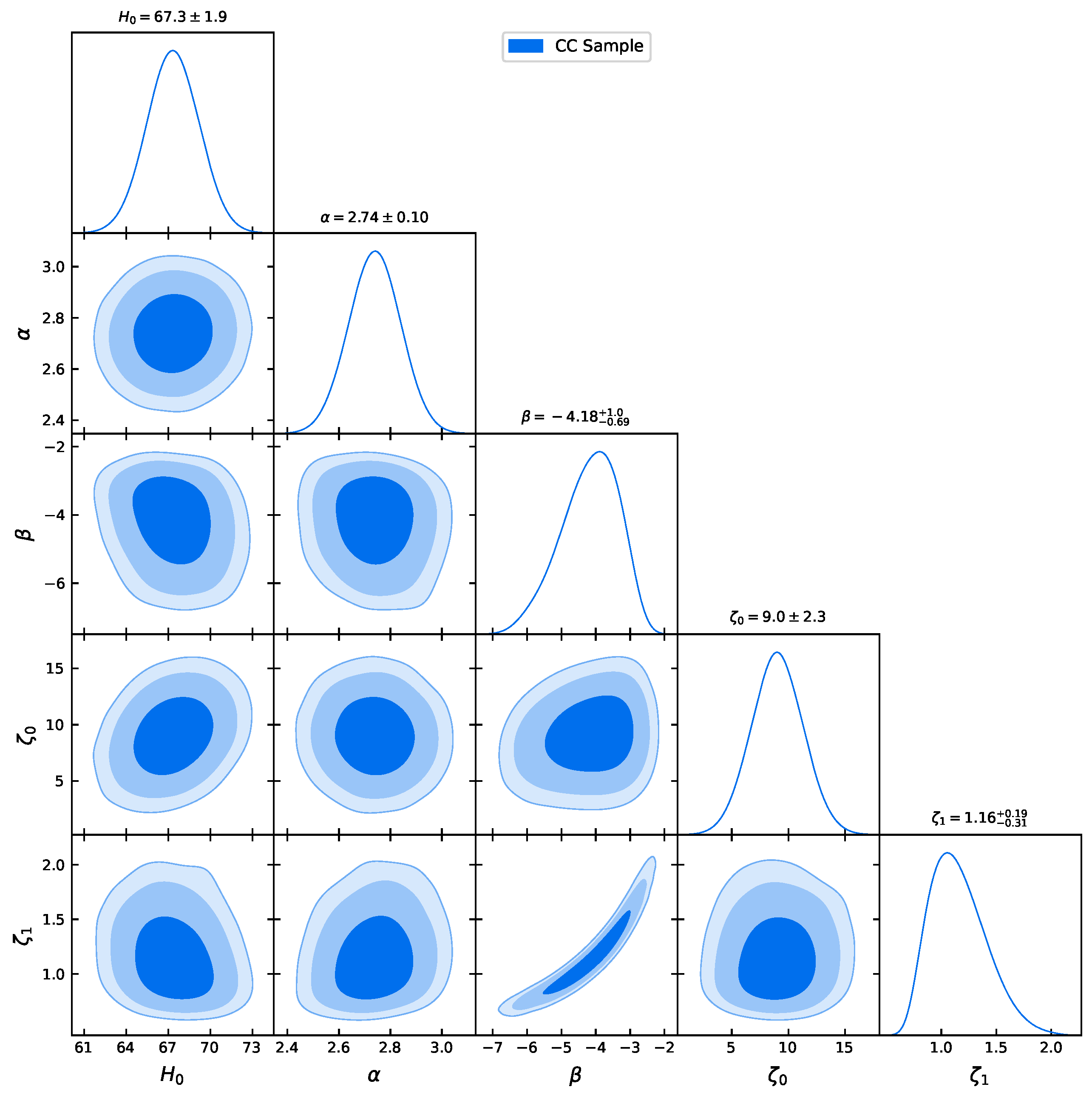
This subsection is dedicated to employ the formulations defined above for each dataset to constrain our model using the MCMC technique. We began with the CC sample by minimizing Equation (
15). The 2D contour results up to
can be observed in
Figure 1, where the innermost region is the confidence level
, the middle region represents the confidence level
, and the outer faded region is the confidence level
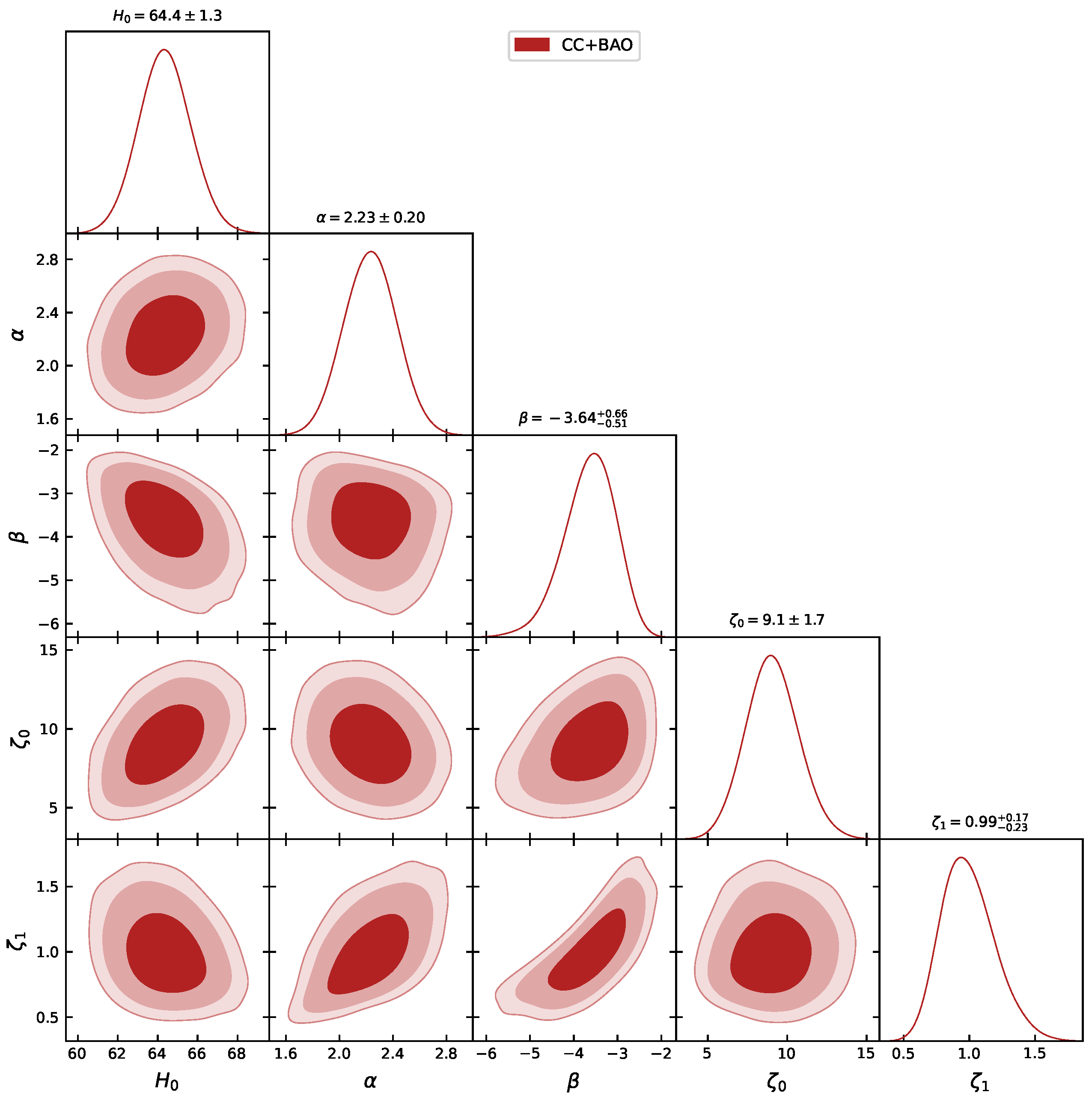
. In addition, we combined the 31 points of the CC with the 26 points of the BAO sample to constrain the linear viscous model. To maximize the likelihood in the MCMC analysis, we considered the sum of Equations (
15) and (
16). The combination gives rise to 2D contours up to
CL, which can be observed in
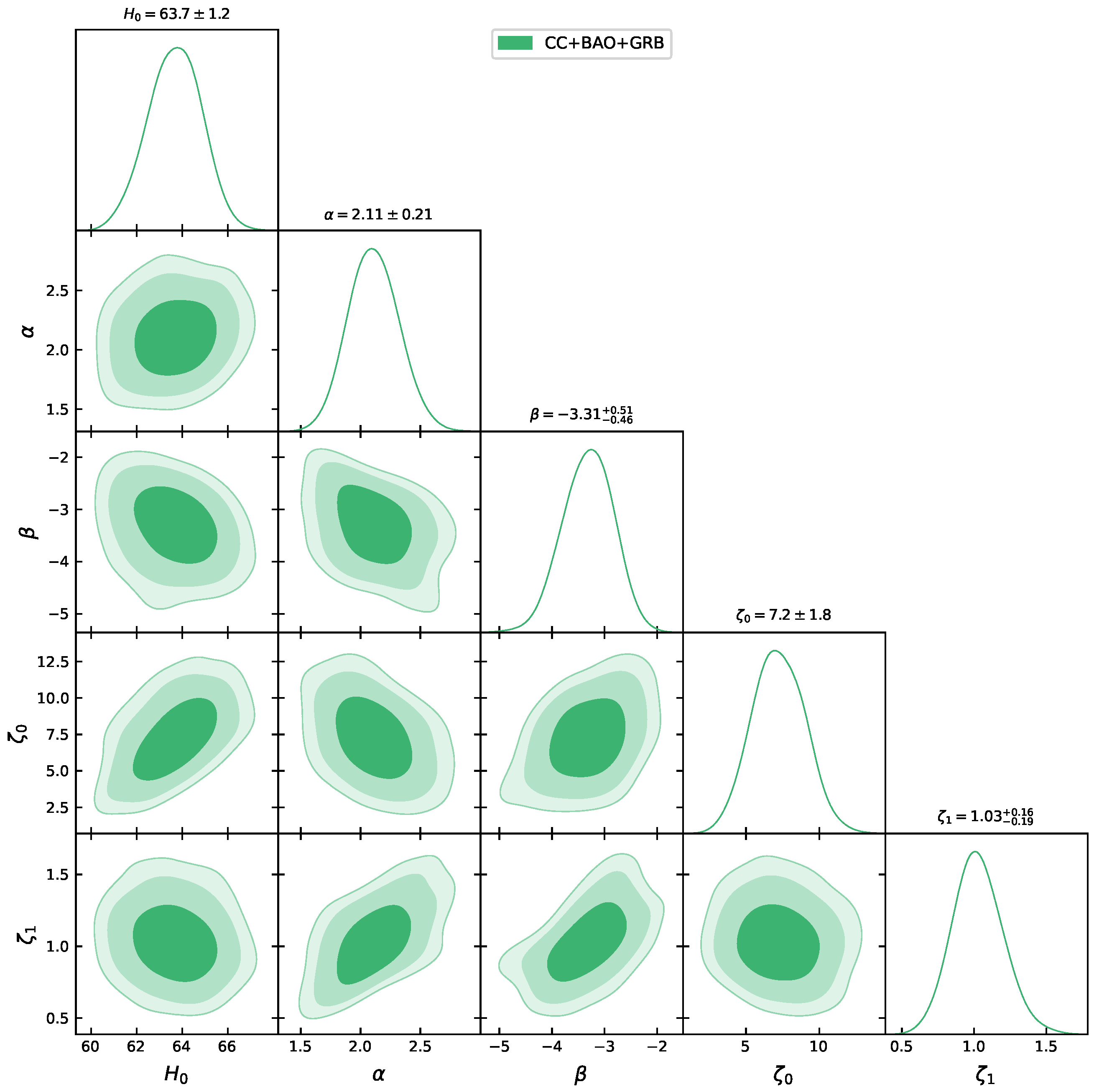
Figure 2. Finally, the 162 points of Gamma-Ray Burst data, which are collected from a wider range of redshift up to 9.3, are combined with the CC and BAO datasets. Following the same methodology, with the Equations (
15), (
16) and (
21), we perform an MCMC simulation to obtain the contours presented in
Figure 3. The respective values of the
ranges are summarized in
Table 1. As seen from
Table 1, although the model parameters obtained from all dataset combinations are numerically close, subtle discrepancies are present. To examine which combination provides greater consistency, we analyze the behavior of the Hubble parameter and the distance modulus functions across the redshift range.
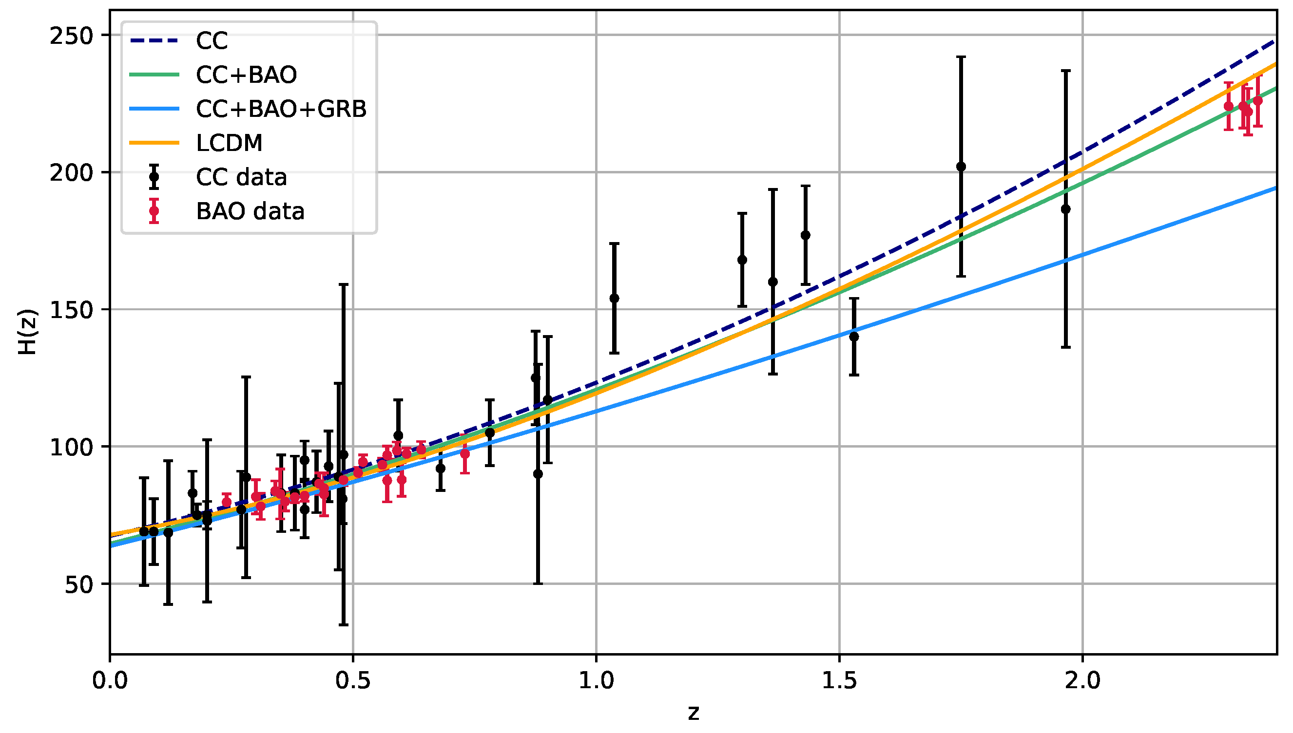
The concordance model, along with the error bars of the datasets, has been considered for comparison purposes with our model. The ability of the concordance model to describe late-time observations is well known. In this context, we consider the Hubble function plot in
Figure 4 and the error bar of the datasets that measure
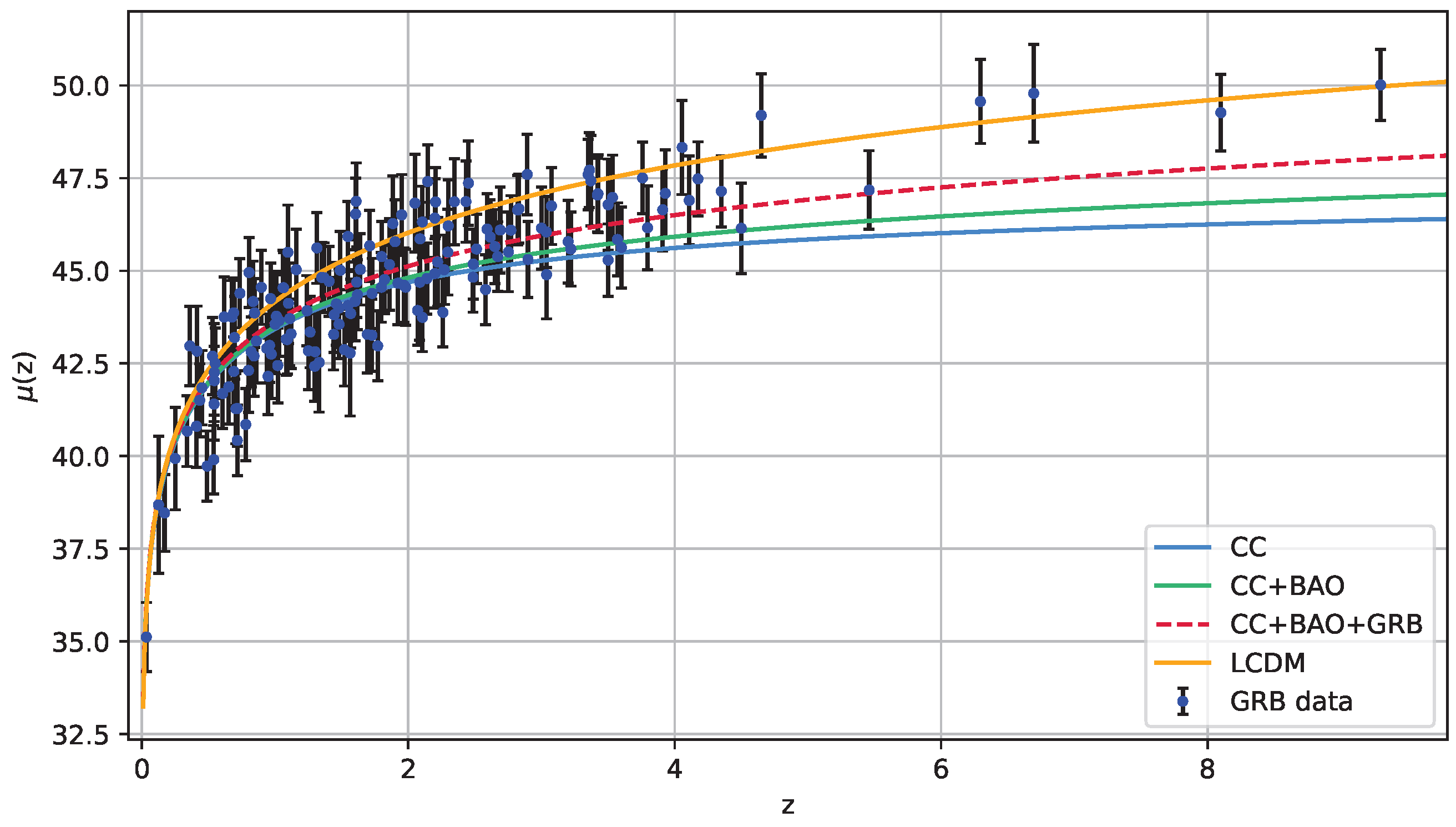
. The curves for our model, obtained from the mean values of the MCMC results are in excellent agreement with the standard cosmological model and the error bars. In addition, we follow the methodology for the distance modulus function against the redshift. As shown in
Figure 5, all model curves exhibit good agreement with the observational data and the
CDM model in the low-redshift regime. At higher redshifts, however, the CC + BAO + GRB combination demonstrates improved consistency with both the standard cosmological model and the GRB data points.
5. Conclusions
In this article, we explored the influence of bulk viscosity on cosmic evolution within the framework of the recently proposed
gravity, where
Q denotes the non-metricity scalar and
represents the matter Lagrangian. In a recent work [
39], the authors successfully reconstructed the
CDM scenario within the
theory.
We commenced with the assumption of the simplest linear form, i.e., , and incorporated a bulk viscous coefficient of the form in our analysis. We derived the analytical solution for the Hubble parameter based on this linear model. This expression, which encapsulates both the model parameters and the viscosity parameters, was subsequently used for Markov Chain Monte Carlo (MCMC) analysis.
The free parameters of the model were constrained using three different combinations of observational data: CC, CC + BAO, and CC + BAO + GRB. The reliability of the results was assessed by comparing them with the predictions of the standard CDM model and the associated observational uncertainties. One of the most noteworthy aspects of the model is its compatibility with both the data and the standard model.
Furthermore, the inclusion of GRB data allows us to extend the analysis into a redshift range that is beyond the reach of conventional probes such as Type Ia supernovae or BAO alone. This highlights the capability of our model to remain viable across a wide range of cosmic epochs, from recent acceleration to early structure formation.
Overall, the agreement of our model with multiple datasets, including high-redshift GRBs, supports its potential as a compelling alternative framework for explaining late-time cosmic acceleration. The model shows promising prospects for future investigations into the cosmic expansion history, structure growth, and possible deviations from the standard paradigm.
Author Contributions
Conceptualization, D.S.R. and S.S.M.; methodology, D.S.R.; software, S.S.M.; validation, D.S.R., S.S.M., A.B., and P.K.S.; formal analysis, D.S.R. and S.S.M.; investigation, D.S.R., S.S.M., A.B., and P.K.S.; resources, D.S.R.; data curation, S.S.M.; writing—original draft preparation, D.S.R. and S.S.M.; writing—review and editing, D.S.R., S.S.M., A.B., and P.K.S.; visualization, P.K.S.; supervision, P.K.S.; project administration, P.K.S. All authors have read and agreed to the published version of the manuscript.
Funding
This research received no external funding.
Data Availability Statement
This article does not include any new dataset.
Acknowledgments
D.S.R. is grateful for the funding received through the Senior Research Fellowship (NTA-UGC-Ref.No.: 211610106591) from the University Grants Commission (UGC). S.S.M. is grateful to the Indian government’s Council of Scientific and Industrial Research (CSIR) for providing the Junior Research Fellowship (E-Certificate No.: JUN21C05815). P.K.S. thanks IUCAA, Pune, India, for its assistance through the visiting associateship program and the Anusandhan National Research Foundation, Department of Science and Technology, Government of India, for financial support to carry out Research project No.: CRG/2022/001847.
Conflicts of Interest
The authors declare no conflicts of interest.
References
- Riess, A.G.; Filippenko, A.V.; Challis, P.; Clocchiatti, A.; Diercks, A.; Garnavich, P.M.; Gilliland, R.L.; Hogan, C.J.; Jha, S.; Kirshner, R.P. Observational Evidence from Supernovae for an Accelerating Universe and a Cosmological Constant. Astron. J. 1998, 116, 1009. [Google Scholar] [CrossRef]
- Perlmutter, S.; Aldering, G.; Goldhaber, G.; Knop, R.A.; Nugent, P.; Castro, P.G.; Deustua, S.; Fabbro, S.; Goobar, A.; Groom, D.E. Measurements of Omega and Lambda from 42 High-Redshift Supernovae. Astrophys. J. 1999, 517, 565. [Google Scholar] [CrossRef]
- Bennett, C.L.; Halpern, M.; Hinshaw, G.; Jarosik, N.; Kogut, A.; Limon, M.; Meyer, S.S.; Page, L.; Spergel, D.N.; Tucker, G.S. First Year Wilkinson Microwave Anisotropy Probe (WMAP) Observations: Preliminary Maps and Basic Results. Astrophys. J. Suppl. 2003, 148, 119–134. [Google Scholar] [CrossRef]
- Spergel, D.N. et al. [WMAP Collaboration] First-year Wilkinson Microwave Anisotropy Probe (WMAP) Observations: Determination of Cosmological Parameters. Astrophys. J. Suppl. 2003, 148, 175. [Google Scholar] [CrossRef]
- Eisenstein, D.J.; Zehavi, I.; Hogg, D.W.; Scoccimarro, R.; Blanton, M.R.; Nichol, R.C.; Scranton, R.; Seo, H.-J.; Tegmark, M.; Zheng, Z. Detection of the Baryon Acoustic Peak In The Large-Scale Correlation Function of SDSS Luminous Red Galaxies. Astrophys. J. 2005, 633, 560. [Google Scholar] [CrossRef]
- Percival, W.J.; Reid, B.A.; Eisenstein, D.J.; Bahcall, N.A.; Budavari, T.; Frieman, J.A.; Fukugita, M.; Gunn, J.E.; Ivezic, Z.; Knapp, G.R. Baryon acoustic oscillations in the Sloan Digital Sky Survey Data Release 7 galaxy sample. Mon. Not. R. Astron. Soc. 2010, 401, 2148. [Google Scholar] [CrossRef]
- Linder, E.V. Einstein’s Other Gravity and the Acceleration of the Universe. Phys. Rev. D 2010, 81, 127301. [Google Scholar] [CrossRef]
- Kavya, N.S.; Mishra, S.S.; Sahoo, P.K.; Venkatesha, V. Can teleparallel f(T) models play a bridge between early and late time Universe? Mon. Not. Roy. Astron. Soc. 2024, 532, 3126–3133. [Google Scholar] [CrossRef]
- Mishra, S.S.; Kavya, N.S.; Sahoo, P.K.; Venkatesha, V. Impact of Teleparallelism on Addressing Current Tensions and Exploring the GW Cosmology. Astrophys. J. 2025, 981, 13. [Google Scholar] [CrossRef]
- Jiménez, J.B.; Heisenberg, L.; Koivisto, T. Coincident General Relativity. Phys. Rev. D 2018, 98, 044048. [Google Scholar] [CrossRef]
- Kolhatkar, A.; Mishra, S.S.; Sahoo, P.K. Investigating early and late-time epochs in “f(Q)” gravity. Eur. Phys. J. C 2024, 84, 888. [Google Scholar] [CrossRef]
- Mishra, S.S.; Bhat, A.; Sahoo, P.K. Probing baryogenesis in f(Q) gravity. Europhys. Lett. 2024, 146, 29001. [Google Scholar] [CrossRef]
- Xu, Y.; Li, G.; Harko, T.; Liang, S. f(Q,T) gravity. Eur. Phys. J. C 2019, 79, 708. [Google Scholar] [CrossRef]
- Kavya, N.S.; Mustafa, G.; Venkatesha, V. Probing the existence of wormhole solutions in f(Q,T) gravity with conformal symmetry. Ann. Phys. 2024, 468, 169723. [Google Scholar] [CrossRef]
- Rathore, S.; Singh, S.S.; Muhammad, S.; Zotos, E.E. Phase space properties of cosmological models in f(Q, T) gravity. Eur. Phys. J. C 2024, 84, 1108. [Google Scholar] [CrossRef]
- Mishra, S.S.; Kavya, N.S.; Sahoo, P.K.; Venkatesha, V. Chebyshev cosmography in the framework of extended symmetric teleparallel theory. Phys. Dark Univ. 2025, 47, 101759. [Google Scholar] [CrossRef]
- Eckart, C. The Thermodynamics of Irreversible Processes. Phys. Rev. 1940, 58, 919. [Google Scholar] [CrossRef]
- Israel, W.; Stewart, J.M. Thermodynamics of nonstationary and transient effects in a relativistic gas. Phys. Lett. B 1976, 58, 213. [Google Scholar] [CrossRef]
- Israel, W. Nonstationary irreversible thermodynamics: A causal relativistic theory. Ann. Phys. 1976, 100, 310. [Google Scholar] [CrossRef]
- Israel, W.; Stewart, J.M. On transient relativistic thermodynamics and kinetic theory. II. Proc. R. Soc. Lond. B 1979, 365, 43. [Google Scholar]
- Brevik, I. Viscosity in modified gravity. Entropy 2012, 14, 2302–2310. [Google Scholar] [CrossRef]
- Brevik, I.; Gron, O. Universe models with negative bulk viscosity. Astrophys. Space Sci. 2013, 347, 399. [Google Scholar] [CrossRef]
- Brevik, I.; Gron, O.; Haro, J.d.; Odintsovd, S.D.; Saridakis, E.N. Viscous Cosmology for Early- and Late-Time Universe. Int. J. Mod. Phys. D 2017, 26, 1730024. [Google Scholar] [CrossRef]
- Brevik, I.; Makarenko, A.N.; Timoshkin, A.V. Viscous accelerating universe with nonlinear and logarithmic equation of state fluid. Int. J. Geom. Methods Mod. 2019, 16, 1950150. [Google Scholar] [CrossRef]
- Brevik, I.; Normann, B.D. Remarks on Cosmological Bulk Viscosity in Different Epochs. Symmetry 2020, 12, 1085. [Google Scholar] [CrossRef]
- Mohan, N.D.J.; Sasidharan, A.; Mathew, T.K. Bulk viscous matter and recent acceleration of the universe based on causal viscous theory. Eur. Phys. J. C 2017, 77, 849. [Google Scholar] [CrossRef]
- Astashenok, A.V.; Odintsov, S.D.; Tepliakov, A.S. The unified history of the viscous accelerating universe and phase transitions. Nucl. Phys. B 2022, 974, 115646. [Google Scholar] [CrossRef]
- Sasidharan, A.; Mathew, T.K. Bulk viscous matter and recent acceleration of the universe. Eur. Phys. J. C 2015, 75, 348. [Google Scholar] [CrossRef]
- Satish, J.; Venkateswarlu, R. Bulk viscous fluid cosmological models in f(R, T) gravity. Chin. J. Phys. 2016, 54, 830–838. [Google Scholar]
- Debnath, P.S. Bulk viscous cosmological model in f(R,T) theory of gravity. Int. J. Geom. Methods Mod. Phys. 2019, 16, 1950005. [Google Scholar] [CrossRef]
- Hazarika, A.; Arora, S.; Sahoo, P.K.; Harko, T. f(Q,Lm) gravity, and its cosmological implications. arXiv 2024, arXiv:2407.00989. [Google Scholar]
- Solanki, R.; Rana, D.S.; Mandal, S.; Sahoo, P.K. Viscous Fluid Cosmology in Symmetric Teleparallel Gravity. Fortschritte Physik. 2023, 71, 2200202. [Google Scholar] [CrossRef]
- Moresco, M. Raising the bar: New constraints on the Hubble parameter with cosmic chronometers at z∼2. Month. Not. R. Astron. Soc. 2015, 450, L16–L20. [Google Scholar] [CrossRef]
- Moresco, M.; Cimatti, A.; Jimenez, R.; Pozzetti, L.; Zamorani, G.; Bolzonella, M.; Dunlop, J.; Lamareille, F.; Mignoli, M.; Pearce, H. Improved constraints on the expansion rate of the Universe up to z∼1.1 from the spectroscopic evolution of cosmic chronometers. J. Cosmol. Astropart. Phys. 2012, 08, 006. [Google Scholar] [CrossRef]
- Moresco, M.; Pozzetti, L.; Cimatti, A.; Jimenez, R.; Maraston, C.; Verde, L.; Thomas, D.; Citro, A.; Tojeiro, R.; Wilkinson, D. A 6% measurement of the Hubble parameter at z∼0.45: Direct evidence of the epoch of cosmic re-acceleration. J. Cosmol. Astropart. Phys. 2016, 05, 014. [Google Scholar] [CrossRef]
- Mishra, S.S.; Kavya, N.S.; Sahoo, P.K.; Venkatesha, V. Constraining Extended Teleparallel Gravity via Cosmography: A Model-independent Approach. Astrophys. J. 2024, 970, 57. [Google Scholar] [CrossRef]
- Amati, L.; Frontera, F.; Tavani, M.; in’t Zand, J.J.M.; Antonelli, A.; Costa, E.; Feroci, M.; Guidorzi, C.; Heise, J.; Masetti, N. Intrinsic spectra and energetics of BeppoSAX Gamma–Ray Bursts with known redshifts. Astron. Astrophys. 2002, 390, 81. [Google Scholar] [CrossRef]
- Demianski, M.; Piedipalumbo, E.; Sawant, D.; Amati, L. Cosmology with gamma-ray bursts I. The Hubble diagram through the calibrated Ep,i − Eiso correlation. Astron. Astrophys. 2017, 598, 14. [Google Scholar] [CrossRef]
- Kavya, N.S.; Venkatesha, V. Embedding the ΛCDM framework in non-minimal f(Q) gravity with matter-coupling. Phys. Lett. B 2024, 856, 138927. [Google Scholar] [CrossRef]
| Disclaimer/Publisher’s Note: The statements, opinions and data contained in all publications are solely those of the individual author(s) and contributor(s) and not of MDPI and/or the editor(s). MDPI and/or the editor(s) disclaim responsibility for any injury to people or property resulting from any ideas, methods, instructions or products referred to in the content. |
© 2025 by the authors. Licensee MDPI, Basel, Switzerland. This article is an open access article distributed under the terms and conditions of the Creative Commons Attribution (CC BY) license (https://creativecommons.org/licenses/by/4.0/).


