
Gamma-Ray Bursts Calibrated by Using Artificial Neural Networks from the Pantheon+ Sample

 , , , , , and
Abstract
1. Introduction
2. Reconstructing the Apparent Magnitude Redshift Relation from Pantheon+ Data
3. Calibration of Amati Relation
4. The GRB Hubble Diagram and Constraints on DE Models
5. Conclusions
Author Contributions
Funding
Data Availability Statement
Acknowledgments
Conflicts of Interest
| 1 | The 2D Dainotti relation [78] is the correlation between the plateau luminosity and its end time in X-ray afterglows; the 3D Dainotti relation [79] is the correlation incorporating the peak prompt luminosity with the plateau end time and luminosity in the rest frame, achieving a small intrinsic scatter. |
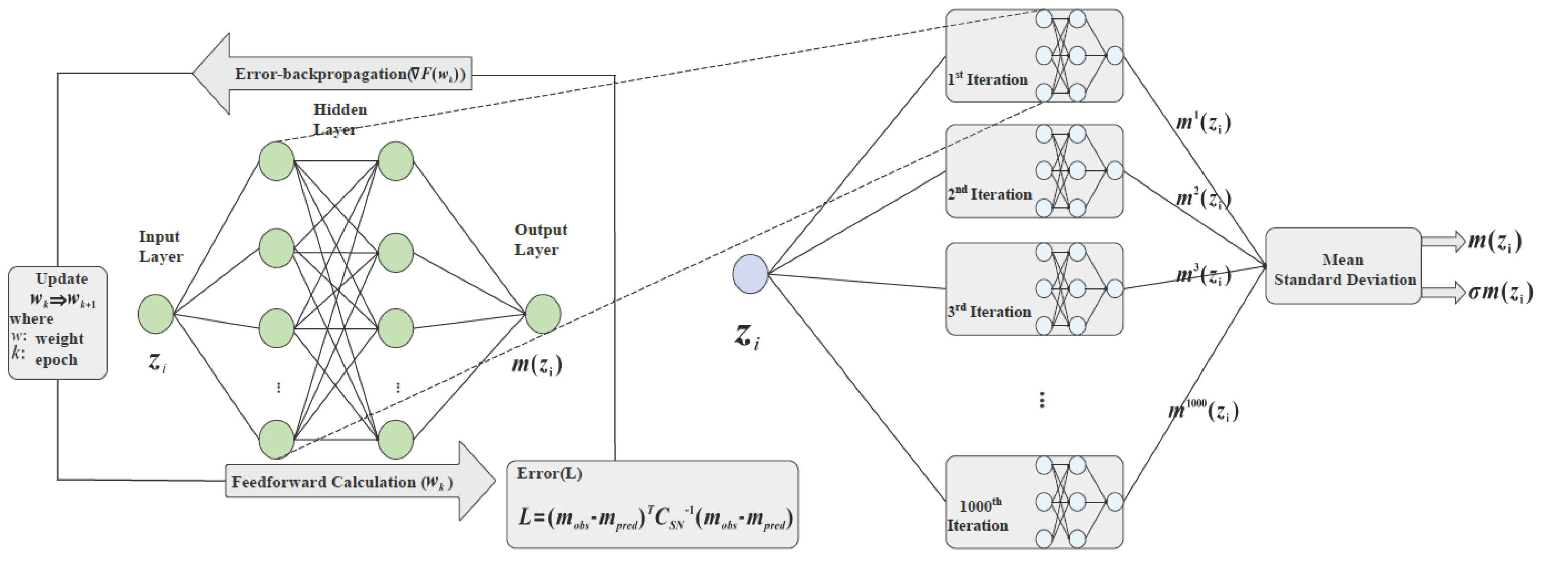
| 2 | We incorporate the Pantheon+ covariance matrix into the loss function: where represents the difference between predicted and observed magnitudes. |
| 3 | The A219 sample is refined from the A220 sample [32] by removing the GRB051109A. |
| 4 | The distance module of SN Ia is related to the luminosity distance and the absolute magnitude (M); the value of M cannot be directly obtained using only the SN Ia sample, and as such M is treated as a free parameter. |
| 5 | Likelihood method of [92]: where and the intrinsic scatter is . |
| 6 | The uncertainty in the apparent magnitude is calculated as follows: where: and , with . |
| 7 | The luminosity distance in a flat universe is expressed as where , and are respectively the matter and DE density parameters, with for flat geometry. For the CDM model, and . |
| 8 |
References
- Dai, Z.; Liang, E.; Xu, D. Constraining ΩM and Dark Energy with Gamma-Ray Bursts. Astrophys. J. 2004, 612, L101. [Google Scholar] [CrossRef]
- Firmani, C.; Ghisellini, G.; Ghirlanda, G.; Avila-Reese, V. A new method optimized to use gamma-ray bursts as cosmic rulers. Mon. Not. R. Astron. Soc. 2005, 360, L1. [Google Scholar] [CrossRef]
- Ghirlanda, G.; Ghisellini, G.; Lazzati, D.; Firmani, C. Gamma-Ray Bursts: New Rulers to Measure the Universe. Astrophys. J. 2004, 613, L13. [Google Scholar] [CrossRef]
- Ghirlanda, G.; Ghisellini, G.; Firmani, C. Gamma-ray bursts as standard candles to constrain the cosmological parameters. New J. Phys. 2006, 8, 123. [Google Scholar] [CrossRef]
- Liang, E.; Zhang, B. Calibration of gamma-ray burst luminosity indicators. Mon. Not. R. Astron. Soc. 2006, 369, L37. [Google Scholar] [CrossRef]
- Schaefer, B.E. Gamma-Ray Burst Hubble Diagram to z = 4.5. Astrophys. J. 2003, 583, L67. [Google Scholar] [CrossRef]
- Schaefer, B.E. The Hubble Diagram to Redshift >6 from 69 Gamma-Ray Bursts. Astrophys. J. 2007, 660, 16. [Google Scholar] [CrossRef]
- Wang, F.; Dai, Z.G. Constraining the cosmological parameters and transition redshift with gamma-ray bursts and supernovae. Mon. Not. R. Astron. Soc. 2006, 368, 371. [Google Scholar] [CrossRef]
- Xu, D.; Dai, Z.; Liang, E. Can Gamma-Ray Bursts Be Used to Measure Cosmology? A Further Analysis. Astrophys. J. 2005, 633, 603. [Google Scholar] [CrossRef]
- Liang, N.; Xiao, W.K.; Liu, Y.; Zhang, S.N. A Cosmology-Independent Calibration of Gamma-Ray Burst Luminosity Relations and the Hubble Diagram. Astrophys. J. 2008, 685, 354. [Google Scholar] [CrossRef]
- Amati, L.; D’Agostino, R.; Luongo, O.; Muccino, M.; Tantalo, M. Addressing the circularity problem in the Ep-Eiso correlation of gamma-ray bursts. Mon. Not. R. Astron. Soc. 2019, 486, L46. [Google Scholar] [CrossRef]
- Amati, L.; Frontera, F.; Tavani, M.; in’t Zand, J.J.M.; Antonelli, A.; Costa, E.; Feroci, M.; Guidorzi, C.; Heise, J.; Masetti, N.; et al. Intrinsic spectra and energetics of BeppoSAX Gamma-Ray Bursts with known redshifts. Astron. Astrophys. 2002, 390, 81. [Google Scholar] [CrossRef]
- Capozziello, S.; Izzo, L. Cosmography by gamma ray bursts. Astron. Astrophys. 2008, 490, 31. [Google Scholar] [CrossRef]
- Capozziello, S.; Izzo, L. Cosmography by GRBs: Gamma Ray Bursts as possible distance indicators. Nucl. Phys. B Proc. Suppl. 2009, 194, 206. [Google Scholar] [CrossRef]
- Demianski, M.; Piedipalumbo, E.; Sawant, D.; Amati, L. Cosmology with gamma-ray bursts. I. The Hubble diagram through the calibrated Ep,I-Eiso correlation. Astron. Astrophys. 2017, 598, A112. [Google Scholar] [CrossRef]
- Demianski, M.; Piedipalumbo, E.; Sawant, D.; Amati, L. Cosmology with gamma-ray bursts. II. Cosmography challenges and cosmological scenarios for the accelerated Universe. Astron. Astrophys. 2017, 598, A113. [Google Scholar] [CrossRef]
- Liang, N.; Wu, P.; Zhang, S.N. Constraints on cosmological models and reconstructing the acceleration history of the Universe with gamma-ray burst distance indicators. Phys. Rev. D 2010, 81, 083518. [Google Scholar] [CrossRef]
- Liang, N.; Xu, L.; Zhu, Z.H. Constraints on the generalized Chaplygin gas model including gamma-ray bursts via a Markov Chain Monte Carlo approach. Astron. Astrophys. 2011, 527, A11. [Google Scholar] [CrossRef]
- Wei, H.; Zhang, S.N. Reconstructing the cosmic expansion history up to redshift z = 6.29 with the calibrated gamma-ray bursts. Eur. Phys. J. C 2009, 63, 139. [Google Scholar] [CrossRef]
- Wei, H. Observational constraints on cosmological models with the updated long gamma-ray bursts. J. Cosmol. Astropart. Phys. 2010, 8, 020. [Google Scholar] [CrossRef]
- Luongo, O.; Muccino, M. Intermediate redshift calibration of gamma-ray bursts and cosmic constraints in non-flat cosmology. Mon. Not. R. Astron. Soc. 2023, 518, 2247. [Google Scholar] [CrossRef]
- Montiel, A.; Cabrera, J.I.; Hidalgo, J.C. Improving sampling and calibration of gamma-ray bursts as distance indicators. Mon. Not. R. Astron. Soc. 2021, 467, 3239. [Google Scholar] [CrossRef]
- Wang, J.S.; Wang, F.Y.; Cheng, K.S.; Dai, Z.G. Measuring dark energy with the Eiso-Ep correlation of gamma-ray bursts using model-independent methods. Astron. Astrophys. 2016, 585, A68. [Google Scholar] [CrossRef]
- Wang, Y.Y.; Wang, F.Y. Calibration of Gamma-Ray Burst Luminosity Correlations Using Gravitational Waves as Standard Sirens. Astrophys. J. 2019, 873, 39. [Google Scholar] [CrossRef]
- Dai, Y.; Zheng, X.-G.; Li, Z.-X.; Gao, H.; Zhu, Z.-H. Redshift evolution of the Amati relation: Calibrated results from the Hubble diagram of quasars at high redshifts. Astron. Astrophys. 2021, 651, L8. [Google Scholar] [CrossRef]
- Purohit, S.; Desai, S. Calibration of Luminosity Correlations of Gamma-Ray Bursts Using Quasars. Galaxies 2024, 12, 69. [Google Scholar] [CrossRef]
- Gowri, G.; Shantanu, D. Low redshift calibration of the Amati relation using galaxy clusters. J. Cosmol. Astropart. Phys. 2022, 10, 69. [Google Scholar] [CrossRef]
- Amati, L.; Guidorzi, C.; Frontera, F.; Della Valle, M.; Finelli, F.; Landi, F.; Montanari, E. Measuring the cosmological parameters with the Ep,i-Eiso correlation of gamma-ray bursts. Mon. Not. R. Astron. Soc. 2008, 391, 577. [Google Scholar] [CrossRef]
- Cao, S.; Dainotti, M.; Ratra, B. Standardizing Platinum Dainotti-correlated gamma-ray bursts, and using them with standardized Amati-correlated gamma-ray bursts to constrain cosmological model parameters. Mon. Not. R. Astron. Soc. 2022, 512, 439. [Google Scholar] [CrossRef]
- Cao, S.; Khadka, N.; Ratra, B. Standardizing Dainotti-correlated gamma-ray bursts, and using them with standardized Amati-correlated gamma-ray bursts to constrain cosmological model parameters. Mon. Not. R. Astron. Soc. 2022, 510, 2928. [Google Scholar] [CrossRef]
- Khadka, N.; Ratra, B. Constraints on cosmological parameters from gamma-ray burst peak photon energy and bolometric fluence measurements and other data. Mon. Not. R. Astron. Soc. 2020, 499, 391. [Google Scholar] [CrossRef]
- Khadka, N.; Luongo, O.; Muccino, M.; Ratra, B. Do gamma-ray burst measurements provide a useful test of cosmological models? J. Cosmol. Astropart. Phys. 2021, 09, 042. [Google Scholar] [CrossRef]
- Cao, S.; Ratra, B. Using lower redshift, non-CMB, data to constrain the Hubble constant and other cosmological parameters. Mon. Not. R. Astron. Soc. 2022, 513, 5686. [Google Scholar] [CrossRef]
- Colgáin, E.O.; Sheikh-Jabbari, M.M.; Yin, L. Do high redshift QSOs and GRBs corroborate JWST? Phys. Dark Universe 2025, 49, 101975. [Google Scholar] [CrossRef]
- Favale, A.; Dainotti, M.G.; Gómez-Valent, A.; Migliaccio, M. Towards a new model-independent calibration of Gamma-Ray Bursts. J. High Energy Astrophys. 2024, 44, 323. [Google Scholar] [CrossRef]
- Han, Y.; Gao, J.; Liu, G.; Xu, L. Detection of gamma-ray burst Amati relation based on Hubble data set and Pantheon+ samples. Eur. Phys. J. C 2024, 84, 934. [Google Scholar] [CrossRef]
- Hu, J.P.; Wang, F.Y.; Dai, Z.G. Measuring cosmological parameters with a luminosity-time correlation of gamma-ray bursts. Mon. Not. R. Astron. Soc. 2021, 507, 730. [Google Scholar] [CrossRef]
- Li, J.-L.; Yang, Y.-P.; Yi, S.-X.; Hu, J.-P.; Qu, Y.-K.; Wang, F.-Y. Standardizing the gamma-ray burst as a standard candle and applying it to cosmological probes: Constraints on the two-component dark energy model. Astron. Astrophys. 2024, 689, A165. [Google Scholar] [CrossRef]
- Liu, Y.; Chen, F.; Liang, N.; Yuan, Z.; Yu, H.; Wu, P. The Improved Amati Correlations from Gaussian Copula. Astrophys. J. 2022, 931, 50. [Google Scholar] [CrossRef]
- Liu, Y.; Liang, N.; Xie, X.; Yuan, Z.; Yu, H.; Wu, P. Gamma-Ray Burst Constraints on Cosmological Models from the Improved Amati Correlation. Astrophys. J. 2022, 935, 7. [Google Scholar] [CrossRef]
- Paliathanasis, A. Testing Non-Coincident f(Q)-gravity with DESI DR2 BAO and GRBs. arXiv 2025, arXiv:2504.11132. [Google Scholar] [CrossRef]
- Tian, X.; Li, J.-L.; Yi, S.-X.; Yang, Y.-P.; Hu, J.-P.; Qu, Y.-K.; Wang, F.-Y. Radio Plateaus in Gamma-Ray Burst Afterglows and Their Application in Cosmology. Astrophys. J. 2023, 958, 74. [Google Scholar] [CrossRef]
- Bargiacchi, G.; Dainotti, M.G.; Hernandez, X. High-redshift cosmology by Gamma-Ray Bursts: An overview. New Astron. Rev. 2025, 100, 101712. [Google Scholar] [CrossRef]
- Deng, C.; Huang, Y.-F.; Xu, F.; Kurban, A. The Observed Luminosity Correlations of Gamma-Ray Bursts and Their Applications. Galaxies 2025, 13, 15. [Google Scholar] [CrossRef]
- Liang, N.; Zhang, S. Cosmology-Independent Distance Moduli of 42 Gamma-Ray Bursts between Redshift of 1.44 and 6.60. AIP Conf. Proc. 2008, 1065, 367–372. [Google Scholar] [CrossRef]
- Kodama, Y.; Yonetoku, D.; Murakami, T.; Tanabe, S.; Tsutsui, R.; Nakamura, T. Gamma-ray bursts in 1.8 < z < 5.6 suggest that the time variation of the dark energy is small. Mon. Not. R. Astron. Soc. 2008, 391, L1. [Google Scholar] [CrossRef]
- Cardone, V.F.; Capozziello, S.; Dainotti, M.G. An updated gamma-ray bursts Hubble diagram. Mon. Not. R. Astron. Soc. 2009, 400, 775. [Google Scholar] [CrossRef]
- Capozziello, S.; Izzo, L. A cosmographic calibration of the Ep,i-Eiso (Amati) relation for GRBs. Astron. Astrophys. 2010, 519, A73. [Google Scholar] [CrossRef]
- Gao, H.; Liang, N.; Zhu, Z.-H. Calibration of GRB Luminosity Relations with Cosmography. Int. J. Mod. Phys. D 2012, 21, 1250016. [Google Scholar] [CrossRef]
- Liu, J.; Wei, H. Cosmological models and gamma-ray bursts calibrated by using Padé method. Gen. Relativ. Gravit. 2015, 47, 141. [Google Scholar] [CrossRef]
- Izzo, L.; Muccino, M.; Zaninoni, E.; Amati, L.; Della Valle, M. New measurements of Ωm from gamma-ray bursts. Astron. Astrophys. 2015, 582, A115. [Google Scholar] [CrossRef]
- Muccino, M.; Izzo, L.; Luongo, O.; Boshkayev, K.; Amati, L.; Della Valle, M.; Pisani, G.B.; Zaninoni, E. Tracing Dark Energy History with Gamma-Ray Bursts. Astrophys. J. 2021, 908, 181. [Google Scholar] [CrossRef]
- Seikel, M.; Clarkson, C.; Smith, M. Reconstruction of dark energy and expansion dynamics using Gaussian processes. J. Cosmol. Astropart. Phys. 2012, 6, 036. [Google Scholar] [CrossRef]
- Li, J.-L.; Yang, Y.-P.; Yi, S.-X.; Hu, J.-P.; Wang, F.-Y.; Qu, Y.-K. Constraints on the Cosmological Parameters with Three-Parameter Correlation of Gamma-Ray Bursts. Astrophys. J. 2023, 953, 58. [Google Scholar] [CrossRef] [PubMed]
- Liang, N.; Li, Z.; Xie, X.; Wu, P. Calibrating Gamma-Ray Bursts by Using a Gaussian Process with Type Ia Supernovae. Astrophys. J. 2022, 941, 84. [Google Scholar] [CrossRef]
- Mu, Y.; Chang, B.; Xu, L. Cosmography via Gaussian process with gamma ray bursts. J. Cosmol. Astropart. Phys. 2023, 9, 041. [Google Scholar] [CrossRef]
- Nong, X.-D.; Liang, N. Testing the Phenomenological Interacting Dark Energy Model with Gamma-Ray Bursts and Pantheon+ type Ia Supernovae. Res. Astron. Astrophys. 2024, 24, 125003. [Google Scholar] [CrossRef]
- Wang, G.Z.; Li, X.L.; Liang, N. Constraining the emergent dark energy models with observational data at intermediate redshift. Astrophys. Space Sci. 2024, 369, 74. [Google Scholar] [CrossRef]
- Wang, H.; Liang, N. Constraints from Fermi observations of long gamma-ray bursts on cosmological parameters. Mon. Not. R. Astron. Soc. 2024, 533, 743. [Google Scholar] [CrossRef]
- Xie, H.; Nong, X.; Wang, H.; Zhang, B.; Li, Z.; Liang, N. Constraints on cosmological models with gamma-ray bursts in cosmology-independent way. Int. J. Mod. Phys. D 2025, 20, 2450073. [Google Scholar] [CrossRef]
- Seikel, M.; Yahya, S.; Maartens, R.; Clarkson, C. Using H(z) data as a probe of the concordance model. Phys. Rev. D 2012, 86, 083001. [Google Scholar] [CrossRef]
- Wei, J.-J.; Wu, X.-F. An Improved Method to Measure the Cosmic Curvature. Astrophys. J. 2017, 838, 160w. [Google Scholar] [CrossRef]
- Zhou, H.; Li, Z. Testing the fidelity of Gaussian processes for cosmography. Chin. Phys. 2019, 43, 035103. [Google Scholar] [CrossRef]
- Luongo, O.; Muccino, M. Model-independent calibrations of gamma-ray bursts using machine learning. Mon. Not. R. Astron. Soc. 2021, 503, 4581. [Google Scholar] [CrossRef]
- Bengaly, C.; Dantas, M.A.; Casarini, L.; Alcaniz, J. Measuring the Hubble constant with cosmic chronometers: A machine learning approach. Eur. Phys. J. 2023, 83, 548. [Google Scholar] [CrossRef]
- Zhang, B.; Wang, H.; Nong, X.; Wang, G.; Wu, P.; Liang, N. Model-independent gamma-ray bursts constraints on cosmological models using machine learning. Astrophys. Space Sci. 2025, 370, 10. [Google Scholar] [CrossRef]
- Scolnic, D.; Brout, D.; Carr, A.; Riess, A.G.; Davis, T.M.; Dwomoh, A.; Jones, D.O.; Ali, N.; Charvu, P.; Chen, R.; et al. The Pantheon+ Analysis: The Full Data Set and Light-curve Release. Astrophys. J. 2022, 938, 113. [Google Scholar] [CrossRef]
- Chen, J.F.; Zhang, T.J.; He, P.; Zhang, T.; Zhang, J. Estimating Cosmological Parameters and Reconstructing Hubble Constant with Artificial Neural Networks: A Test with covariance matrix and mock H(z). arXiv 2024, arXiv:2410.08369. [Google Scholar] [CrossRef]
- Dialektopoulos, K.; Said, J.L.; Mifsud, J.; Sultana, J.; Adami, K.Z. Neural network reconstruction of late-time cosmology and null tests. J. Cosmol. Astropart. Phys. 2022, 2, 023. [Google Scholar] [CrossRef]
- Di Valentino, E.; Levi Said, J.; Riess, A.; Pollo, A.; Poulin, V.; Gómez-Valent, A.; Weltman, A.; Palmese, A.; Huang, C.; van de Bruck, C.; et al. The CosmoVerse White Paper: Addressing observational tensions in cosmology with systematics and fundamental physics. arXiv 2025, arXiv:2405.19953. [Google Scholar] [CrossRef]
- Escamilla-Rivera, C.; Quintero, M.A.C.; Capozziello, S. A deep learning approach to cosmological dark energy models. J. Cosmol. Astropart. Phys. 2020, 3, 008. [Google Scholar] [CrossRef]
- Gómez-Vargas, I.; Medel-Esquivel, R.; García-Salcedo, R.; Vázquez, J.A. Neural network reconstructions for the Hubble parameter, growth rate and distance modulus. Eur. Phys. J. C 2023, 83, 304. [Google Scholar] [CrossRef]
- Niu, J.; He, P.; Zhang, T.-J. Constraining the Hubble Constant with a Simulated Full Covariance Matrix Using Neural Networks. arXiv 2025, arXiv:2502.11443. [Google Scholar] [CrossRef]
- Wang, G.-J.; Ma, X.-J.; Li, S.-Y.; Xia, J.-Q. Reconstructing Functions and Estimating Parameters with Artificial Neural Networks: A Test with a Hubble Parameter and SNe Ia. Astrophys. J. Suppl. Ser. 2020, 246, 13. [Google Scholar] [CrossRef]
- Zhang, J.C.; Hu, Y.; Jiao, K.; Wang, H.F.; Xie, Y.B.; Yu, B.; Zhao, L.L.; Zhang, T.J. A Nonparametric Reconstruction of the Hubble Parameter H(z) Based on Radial Basis Function Neural Networks. Astrophys. J. Suppl. Ser. 2024, 270, 23. [Google Scholar] [CrossRef]
- Shah, R.; Saha, S.; Mukherjee, P.; Garain, U.; Pal, S. LADDER: Revisiting the Cosmic Distance Ladder with Deep Learning Approaches and Exploring Its Applications. Astrophys. J. Suppl. Ser. 2024, 273, 27. [Google Scholar] [CrossRef]
- Mukherjee, P.; Dainotti, M.; Dialektopoulos, K.F.; Said, J.L.; Mifsud, J. Model-independent calibration of Gamma-Ray Bursts with neural networks. arXiv 2024, arXiv:2411.03773. [Google Scholar] [CrossRef]
- Dainotti, M.G.; Cardone, V.F.; Capozziello, S. A time-luminosity correlation for γ-ray bursts in the X-rays. Mon. Not. R. Astron. Soc. 2008, 391, L79. [Google Scholar] [CrossRef]
- Dainotti, M.G.; Postnikov, S.; Hernandez, X.; Ostrowski, M. A Fundamental Plane for Long Gamma-Ray Bursts with X-Ray Plateaus. Astrophys. J. 2016, 825, L20. [Google Scholar] [CrossRef]
- Huang, Z.; Xiong, Z.; Luo, X.; Wang, G.; Liu, Y.; Liang, N. Gamma-ray bursts calibrated from the observational H(z) data in artificial neural network framework. J. High Energy Astrophys. 2025, 47, 100337. [Google Scholar] [CrossRef]
- Cao, S.; Ratra, B. Testing the standardizability of, and deriving cosmological constraints from, a new Amati-correlated gamma-ray burst data compilation. J. Cosmol. Astropart. Phys. 2024, 10, 093. [Google Scholar] [CrossRef]
- Jia, X.D.; Hu, J.P.; Yang, J.; Zhang, B.B.; Wang, F.Y. E iso-Ep correlation of gamma-ray bursts: Calibration and cosmological applications. Mon. Not. R. Astron. Soc. 2022, 516, 2575. [Google Scholar] [CrossRef]
- Escamilla-Rivera, C.; Carvajal, M.; Zamora, C.; Hendry, M. Neural networks and standard cosmography with newly calibrated high redshift GRB observations. J. Cosmol. Astropart. Phys. 2022, 4, 016. [Google Scholar] [CrossRef]
- Tang, L.; Li, X.; Lin, H.-N.; Liu, L. Model-independently Calibrating the Luminosity Correlations of Gamma-Ray Bursts Using Deep Learning. Astrophys. J. 2021, 907, 121. [Google Scholar] [CrossRef]
- Tang, L.; Lin, H.-N.; Li, X.; Liu, L. Reconstructing the Hubble diagram of gamma-ray bursts using deep learning. Mon. Not. R. Astron. Soc. 2022, 509, 1194. [Google Scholar] [CrossRef]
- Rumelhart, D.E.; Hinton, G.E.; Williams, R.J. Learning representations by back-propagating errors. Nature 1986, 323, 533. [Google Scholar] [CrossRef]
- Gal, Y.; Ghahramani, Z. Dropout as a Bayesian Approximation: Representing Model Uncertainty in Deep Learning. arXiv 2016, arXiv:1506.02142. [Google Scholar] [CrossRef]
- Gal, Y.; Ghahramani, Z. Dropout as a Bayesian Approximation: Appendix. arXiv 2016, arXiv:1506.02157. [Google Scholar] [CrossRef]
- Srivastava, N.; Hinton, G.; Krizhevsky, A.; Sutskever, I.; Salakhutdinov, R. Dropout: A Simple Way to Prevent Neural Networks from Overftting. J. Mach. Learn. Res. 2014, 15, 1929. [Google Scholar]
- Zhang, H.; Liu, Y.; Yu, H.; Nong, X.; Liang, N.; Wu, P. Constraints on cosmological models from quasars calibrated with type Ia supernova by a Gaussian process. Mon. Not. R. Astron. Soc. 2024, 530, 4493. [Google Scholar] [CrossRef]
- Foreman-Mackey, D.; Hogg, D.W.; Lang, D.; Goodman, J. emcee: The MCMC Hammer. Publ. Astron. Soc. Pac. 2013, 125, 306. [Google Scholar] [CrossRef]
- Reichart, D.E. Dust Extinction Curves and Lyα Forest Flux Deficits for Use in Modeling Gamma-Ray Burst Afterglows and All Other Extragalactic Point Sources. Astrophys. J. 2001, 553, 57. [Google Scholar] [CrossRef]
- Amati, L.; Della Valle, M. Measuring Cosmological Parameters with Gamma Ray Bursts. Int. J. Mod. Phys. 2013, 22, 1330028. [Google Scholar] [CrossRef]
- Li, Z.; Zhang, B.; Liang, N. Testing dark energy models with gamma-ray bursts calibrated from the observational H(z) data through a Gaussian process. Mon. Not. R. Astron. Soc. 2023, 521, 4406. [Google Scholar] [CrossRef]
- Demianski, M.; Piedipalumbo, E.; Sawant, D.; Amati, L. Prospects of high redshift constraints on dark energy models with the Ep,i-Eiso correlation in long gamma ray bursts. Mon. Not. R. Astron. Soc. 2021, 506, 903. [Google Scholar] [CrossRef]
- Kumar, D.; Rani, N.; Jain, D.; Mahajan, S.; Mukherjee, A. Gamma rays bursts: A viable cosmological probe? J. Cosmol. Astropart. Phys. 2023, 07, 021. [Google Scholar] [CrossRef]
- Lin, H.N.; Li, X.; Chang, Z. Model-independent distance calibration of high-redshift gamma-ray bursts and constrain on the ΛCDM model. Mon. Not. R. Astron. Soc. 2016, 455, 2131. [Google Scholar] [CrossRef]
- Wang, G.-J.; Wei, J.-J.; Li, Z.-X.; Xia, J.-Q.; Zhu, Z.-H. Model-independent Constraints on Cosmic Curvature and Opacity. Astrophys. J. 2017, 847, 45. [Google Scholar] [CrossRef]
- Chevallier, M.; Polarski, D. Accelerating Universes with Scaling Dark Matter. Int. J. Mod. Phys. D 2001, 10, 213. [Google Scholar] [CrossRef]
- Linder, E.V. Exploring the Expansion History of the Universe. Phys. Rev. Lett. 2003, 90, 091301. [Google Scholar] [CrossRef]
- Moresco, M.; Cimatti, A.; Jimenez, R.; Pozzetti, L.; Zamorani, G.; Bolzonella, M.; Dunlop, J.; Lamareille, F.; Mignoli, M.; Pearce, H.; et al. Improved constraints on the expansion rate of the Universe up to z ~1.1 from the spectroscopic evolution of cosmic chronometers. J. Cosmol. Astropart. Phys. 2012, 2012, 006. [Google Scholar] [CrossRef]
- Moresco, M. Raising the bar: New constraints on the Hubble parameter with cosmic chronometers at z ~2. Mon. Not. R. Astron. Soc. 2015, 450, L16. [Google Scholar] [CrossRef]
- Moresco, M.; Pozzetti, L.; Cimatti, A.; Jimenez, R.; Maraston, C.; Verde, L.; Thomas, D.; Citro, A.; Tojeiro, R.; Wilkinson, D. A 6% measurement of the Hubble parameter at z~0.45: Direct evidence of the epoch of cosmic re-acceleration. J. Cosmol. Astropart. Phys. 2016, 2016, 014. [Google Scholar] [CrossRef]
- Ratsimbazafy, A.L.; Loubser, S.I.; Crawford, S.M.; Cress, C.M.; Bassett, B.A.; Nichol, R.C.; Väisänen, P. Age-dating luminous red galaxies observed with the Southern African Large Telescope. Mon. Not. R. Astron. Soc. 2017, 467, 3239. [Google Scholar] [CrossRef]
- Stern, D.; Jimenez, R.; Verde, L.; Kamionkowski, M.; Starford, S.A. Cosmic chronometers: Constraining the equation of state of dark energy. I: H(z) measurements. J. Cosmol. Astropart. Phys. 2010, 2010, 008. [Google Scholar] [CrossRef]
- Zhang, C.; Zhang, H.; Yuan, S.; Liu, S.; Zhang, T.; Sun, Y. Four new observational H(z) data from luminous red galaxies in the Sloan Digital Sky Survey data release seven. Res. Astron. Astrophys. 2014, 14, 1221. [Google Scholar] [CrossRef]
- Jiao, K.; Borghi, N.; Moresco, M.; Zhang, T.-J. New Observational H(z) Data from Full-spectrum Fitting of Cosmic Chronometers in the LEGA-C Survey. Astrophys. J. Suppl. Ser. 2023, 265, 48. [Google Scholar] [CrossRef]
- Borghi, N.; Moresco, M.; Cimatti, A. Toward a Better Understanding of Cosmic Chronometers: A New Measurement of H(z) at z∼0.7. Astrophys. J. 2022, 928, L4. [Google Scholar] [CrossRef]
- Moresco, M.; Jimenez, R.; Verde, L.; Cimatti, A.; Pozzetti, L. Setting the Stage for Cosmic Chronometers. II. Impact of Stellar Population Synthesis Models Systematics and Full Covariance Matrix. Astrophys. J. 2020, 898, 82. [Google Scholar] [CrossRef]
- Aghanim, N.; Akrami, Y.; Arroja, F.; Ashdown, M.; Aumont, J.; Baccigalupi, C.; Ballardini, M.; Banday, A.J.; Barreiro, R.B.; Bartolo, N.; et al. Planck 2018 results. I. Overview and the cosmological legacy of Planck. Astron. Astrophys. 2020, 641, A1. [Google Scholar] [CrossRef]
- Titarchuk, L.; Farinelli, R.; Frontera, F.; Amati, L. An Upscattering Spectral Formation Model for the Prompt Emission of Gamma-Ray Bursts. Astrophys. J. 2012, 752, 116. [Google Scholar] [CrossRef]
- Frontera, F.; Amati, L.; Guidorzi, C.; Landi, R.; in’t Zand, J. Broadband Time-resolved E p,i-L iso Correlation in Gamma-Ray Bursts. Astrophys. J. 2012, 754, 138. [Google Scholar] [CrossRef]
- Cao, S.; Ratra, B. Testing the consistency of new Amati-correlated gamma-ray burst dataset cosmological constraints with those from better-established cosmological data. arXiv 2025, arXiv:2502.08429. [Google Scholar] [CrossRef]


| Hyperparameter | Candidate Values | |
|---|---|---|
| Batch size | 16, 32, 64 | |
| Hidden layers | Layers | Units |
| 1 | 64, 128, 256, 512 | |
| 2 | (64, 32), (128, 64) | |
| 3 | (256, 128, 64), (512, 256, 128) | |
| Activate function | ReLU, Sigmoid, Tanh | |
| Dropout rate | 0.1, 0.2, 0.3, 0.4, 0.5 | |
| Methods | Datasets | b | ||
|---|---|---|---|---|
| ANN | 79 GRBs () | |||
| GaPP | 79 GRBs () |
| Models | Method | Data Sets | h | ||||||
|---|---|---|---|---|---|---|---|---|---|
| CDM | ANN | 140 GRBs | - | - | - | 53.059 | - | - | |
| GaPP | 140 GRBs | - | - | - | 40.402 | - | - | ||
| ANN | 140 GRBs + 32 OHD | - | - | 78.576 | - | - | |||
| GaPP | 140 GRBs + 32 OHD | - | - | 80.785 | - | - | |||
| CPL | ANN | 140 GRBs | - | 53.158 | 3.901 | 9.784 | |||
| GaPP | 140 GRBs | - | 40.407 | 3.995 | 9.879 | ||||
| ANN | 140 GRBs + 32 OHD | 78.953 | 3.622 | 9.917 | |||||
| GaPP | 140 GRBs + 32 OHD | 81.227 | 3.554 | 9.848 |
Disclaimer/Publisher’s Note: The statements, opinions and data contained in all publications are solely those of the individual author(s) and contributor(s) and not of MDPI and/or the editor(s). MDPI and/or the editor(s) disclaim responsibility for any injury to people or property resulting from any ideas, methods, instructions or products referred to in the content. |
© 2025 by the authors. Licensee MDPI, Basel, Switzerland. This article is an open access article distributed under the terms and conditions of the Creative Commons Attribution (CC BY) license (https://creativecommons.org/licenses/by/4.0/).
Share and Cite
Huang, Z.; Luo, X.; Zhang, B.; Feng, J.; Wu, P.; Liu, Y.; Liang, N. Gamma-Ray Bursts Calibrated by Using Artificial Neural Networks from the Pantheon+ Sample. Universe 2025, 11, 241. https://doi.org/10.3390/universe11080241
Huang Z, Luo X, Zhang B, Feng J, Wu P, Liu Y, Liang N. Gamma-Ray Bursts Calibrated by Using Artificial Neural Networks from the Pantheon+ Sample. Universe. 2025; 11(8):241. https://doi.org/10.3390/universe11080241
Chicago/Turabian StyleHuang, Zhen, Xin Luo, Bin Zhang, Jianchao Feng, Puxun Wu, Yu Liu, and Nan Liang. 2025. "Gamma-Ray Bursts Calibrated by Using Artificial Neural Networks from the Pantheon+ Sample" Universe 11, no. 8: 241. https://doi.org/10.3390/universe11080241
APA StyleHuang, Z., Luo, X., Zhang, B., Feng, J., Wu, P., Liu, Y., & Liang, N. (2025). Gamma-Ray Bursts Calibrated by Using Artificial Neural Networks from the Pantheon+ Sample. Universe, 11(8), 241. https://doi.org/10.3390/universe11080241