Constraints on Lorentz Invariance Violation from Gamma-Ray Burst Rest-Frame Spectral Lags Using Profile Likelihood

Abstract

We reanalyze the spectral lag data for 56 Gamma-Ray Bursts (GRBs) in the cosmological rest frame to search for Lorentz Invariance Violation (LIV) using frequentist inference. For this purpose, we use the technique of profile likelihood to deal with the nuisance parameters, corresponding to a constant time lag in the GRB rest frame and an unknown intrinsic scatter, while the parameter of interest is the energy scale for LIV ($E_{QG}$). With this method, we do not obtain a global minimum for ${\chi }^2$ as a function of $E_{QG}$ up to the Planck scale. Thus, we can obtain one-sided lower limits on $E_{QG}$ in a seamless manner. Therefore, the 95% c.l. lower limits which we thus obtain on $E_{QG}$ are then given by $E_{QG}\ge 2.07\times {10}^{14}$ GeV and $E_{QG}\ge 3.71\times {10}^5$ GeV, for linear and quadratic LIV, respectively.

1. Introduction

Spectral lags of Gamma-Ray Bursts (GRBs) have been widely used as a probe of Lorentz Invariance Violation (LIV) [1,2,3]. The spectral lag is defined as the time difference between the arrival of high-energy and low-energy photons and is considered to be positive if the high-energy photons precede the low-energy ones. In the case of LIV caused by an energy-dependent slowdown of the speed of light, one expects a turnover in the spectral lag data at higher energies.

Most of the searches for LIV using GRB spectral lags have been carried out using fixed-energy intervals in the observer frame. The first work to search for LIV using spectral lags between fixed rest-frame energy bands was the analysis in Wei and Wu [4] (W17, hereafter). This work considered a sample of 56 Swift-BAT detected GRBs, with spectral lags in the fixed rest-frame energy bands 100–150 keV and 200–250 keV [5]. Based on a Bayesian analysis, W17 obtained a robust lower limit on the LIV energy scale, $E_{QG}\ge 2.2\times {10}^{14}$ GeV at 95% credible intervals.

In the recent two decades, Bayesian statistics has become the industry standard for parameter inference in almost all areas of astrophysics and cosmology [6], including in searches for LIV. However, there has been a renaissance in the use of frequentist statistics in the field of cosmology, over the past 2–3 years, where the nuisance parameters were dispensed with using profile likelihood [7,8,9,10,11]. Some of the advantages and disadvantages of profile likelihood as compared to Bayesian analysis have been reviewed in the aforementioned works.

In this work, we redo the analysis in W17 using frequentist analysis, where we once again deal with nuisance parameters using profile likelihood. This manuscript is structured as follows. The analysis methodology is described in Section 2. Our results are discussed in Section 3, and we summarize our conclusions in Section 4.

2. Analysis Methodology

We briefly recap the equations used for the analysis of LIV following the same prescription and assumptions as in W17. The observed spectral time lag ($\mathrm{\Delta }{t}_{obs}$) from a given GRB at a redshift z can be written down as

$${\displaystyle \frac{\mathrm{\Delta }{t}_{obs}}{1+z}}=a_{LIV}K+\langle b\rangle ,$$

(1)

where $a_{LIV}K$ is given by the following expression for superluminal LIV [12] as follows:

$$a_{LIV}K={\displaystyle \frac{1+n}{2H_0}}{\displaystyle \frac{E_h^n-E_l^n}{{(1+z)}^n{E}_{QG,n}^n}}{\int }_0^z{\displaystyle \frac{{(1+z^{\prime })}^{n}d{z}^{\prime }}{\sqrt{{\mathrm{\Omega }}_M{(1+z^{\prime })}^3+1-{\mathrm{\Omega }}_M}}},$$

(2)

where n indicated the order of LIV and is equal to 1 and 2 for linear and quadratic LIV, respectively; ${\mathrm{\Omega }}_M$ and $H_0$ are the cosmological parameters corresponding to the matter density and Hubble constant, respectively. We used the same values for the cosmological parameters as W17 (viz. ${\mathrm{\Omega }}_M=0.308$ and $H_0=67.8$ km/s/Mpc). The energies $E_h$ and $E_l$ correspond to the energies in the rest-frame bands, from which the spectral lags were obtained with $E_h>E_l$. The second term in Equation (1), namely $\langle b\rangle$, represents the average effect of intrinsic time lags (due to astrophysics), as discussed in W17. Although a large number of phenomenological models have been used to model the intrinsic spectral lag [1], here we model the astrophysical lag by a constant term similar to W17 for a straightforward comparison.

Similar to W17, we fit the observable ${\displaystyle \frac{\mathrm{\Delta }{t}_{obs}}{1+z}}$ to Equation (1) using maximum likelihood estimation and by adding an additional intrinsic scatter (${\sigma }_{int}$) to the observed uncertainties in the spectral lags

$$\mathcal{L}(E_{QG},{\sigma }_{int},\langle b\rangle )={\displaystyle \prod _{i=1}^N}{\displaystyle \frac{1}{\sqrt{{\left(\frac{{\sigma }_i}{1+z}\right)}^2+{\sigma }_{int}^2}}}exp\left\{-{\displaystyle \frac{{\left(\frac{\mathrm{\Delta }{t}_{obs}}{1+z}-a_{LIV}K-\langle b\rangle \right)}^2}{2\left({\sigma }_{int}^2+{\left(\frac{{\sigma }_i}{1+z}\right)}^2\right)}}\right\},$$

(3)

where ${\sigma }_i$ is the uncertainty in $\mathrm{\Delta }{t}_{obs}$, and ${\sigma }_{int}$ is the unknown intrinsic scatter, which we fit for. Therefore, our regression problem contains three unknown parameters: $E_{QG}$, $\langle b\rangle$, and ${\sigma }_{int}$. In this problem, $\langle b\rangle$ and ${\sigma }_{int}$ represent the nuisance parameters, which we account for using profile likelihood to obtain the likelihood distribution as a function of $E_{QG}$:

$$\mathcal{L}\left(E_{QG}\right)=\underset{{\sigma }_{int},\langle b\rangle }{max}\mathcal{L}(E_{QG},{\sigma }_{int},\langle b\rangle )$$

(4)

For ease of computation, instead of maximizing Equation (4), we construct ${\chi }^2$ which is defined as

$${\chi }^2\equiv -2lnL(E_{QG},{\sigma }_{int},\langle b\rangle )$$

(5)

We then minimize ${\chi }^2$ defined in Equation (5) over ${\sigma }_{int}$ and $\langle b\rangle$ for a fixed value of $E_{QG}$. We then obtain frequentist confidence intervals (or upper limits) on $E_{QG}$ from $\mathrm{\Delta }{\chi }^2\left(E_{QG}\right)={\chi }^2\left(E_{QG}\right)-{\chi }_{min}^2$, where ${\chi }_{min}^2$ is the global minimum for ${\chi }^2$ over all values of $E_{QG}$. For this purpose, we use Wilks’ theorem, which states that $\mathrm{\Delta }{\chi }^2$ follows a ${\chi }^2$ distribution for one degree of freedom [13].

3. Results

We now apply the methodology in the previous section to the spectral lag data of 56 Swift-BAT detected GRBs, consisting of both short and long GRBs collated in Bernardini et al. [5], where the spectral lags were calculated in fixed rest-frame energy bands of 100–150 keV and 200–250 keV. This dataset consists of GRBs with redshifts ranging from 0.35 (GRB 061021) to 5.47 (GRB 060927), having a mean redshift of 1.73. The energy gap between the midpoints of the successive rest-frame energy intervals is fixed at 100 keV. The uncertainties in the spectral delay are calculated by averaging the left and right uncertainties provided in the aforementioned work. The full details of the 56 GRBs used for the analysis, such as the GRB name, redshift, observed spectral lags, and their uncertainties, can be found in Table 1 of Bernardini et al. [5].

To evaluate profile likelihood, we construct a logarithmically spaced grid for $E_{QG}$ from ${10}^5$ GeV to ${10}^{19}$ GeV for linear and quadratic models of LIV. The upper bound of ${10}^{19}$ GeV corresponds to the Planck scale. For each value of $E_{QG}$, we calculate the minimum value of ${\chi }^2\left(E_{QG}\right)$ by minimizing over ${\sigma }_{int}$ and $\langle b\rangle$. This minimization was carried out using the scipy.optimize.fmin function, which uses the Nelder–Mead simplex algorithm [14]. We also cross-checked this result with other minimization algorithms available in scipy and found that the results do not change.

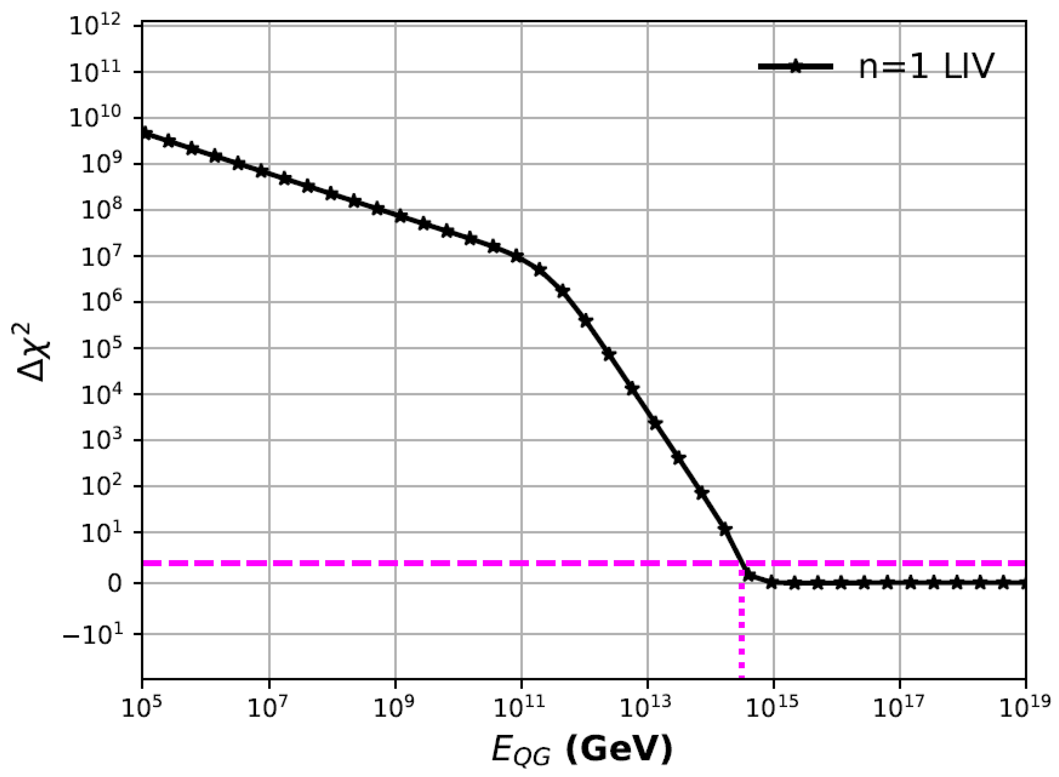
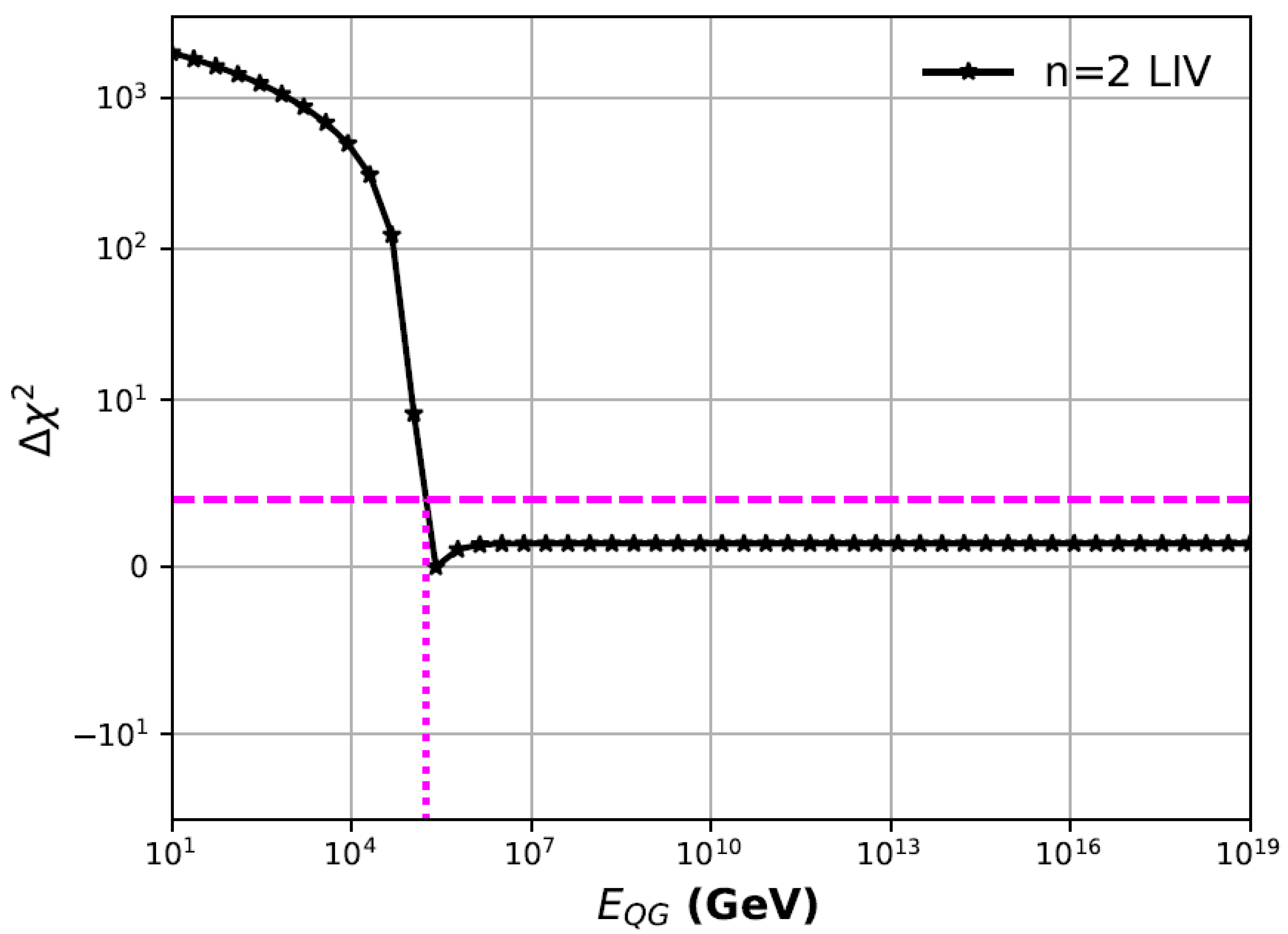
We find that ${\chi }^2$ does not achieve global minima below the Planck scale ($E_{pl}$). We then plot the curves of $\mathrm{\Delta }{\chi }^2$ as a function of $E_{QG}$ for the linear and quadratic models of LIV, where $\mathrm{\Delta }{\chi }^2={\chi }^2\left(E_{QG}\right)-{\chi }^2\left(E_{pl}\right)$. These $\mathrm{\Delta }{\chi }^2$ curves can found in Figure 1 and Figure 2, for linear and quadratic models of LIV, respectively. Since we do not obtain global minima below the Planck scale, we can set one-sided 95.4% confidence level (c.l.) lower limits, by finding the x-intercept for which $\mathrm{\Delta }{\chi }^2=4$. For brevity, we denote 95.4% c.l. as 95% c.l. These 95% c.l. lower limits are given by $E_{QG}\ge 2.07\times {10}^{14}$ GeV and $E_{QG}\ge 3.71\times {10}^5$ GeV, for linear and quadratic LIV, respectively. Therefore, we can set lower limits on the energy scale of LIV in a seamless manner, since we do not obtain a global minimum. Since our main aim was to compare our results to W17, we used the same cosmological parameters as those in W17. When we vary the cosmological parameters and use the latest values from PDG, viz. $H_0=67.4$ km/s and ${\mathrm{\Omega }}_m=0.315$, we do not find qualitative differences in the shape of ${\chi }^2$ as a function of $E_{QG}$. The new 95% lower limits on $E_{QG}$ change to $E_{QG}\ge 2.08\times {10}^{14}$ GeV and $E_{QG}\ge 3.71\times {10}^5$ GeV, for linear and quadratic LIV, respectively. Therefore, the variation in the lower limit on $E_{QG}$ is negligible upon choosing the PDG cosmological parameters.

In order to judge the efficacy of the fit, similar to W17, we calculate the ${\chi }_{fit}^2$ based on the residuals between the data and best-fit model, as follows:

$${\chi }_{fit}^2=\sum _i{\displaystyle \frac{{\left(\frac{\mathrm{\Delta }{t}_i}{1+z_i}-a_{\mathrm{LIV}}{K}_i-\langle b\rangle \right)}^2}{{\sigma }_{\mathrm{int}}^2+{\left(\frac{{\sigma }_i}{1+z_i}\right)}^2}}.$$

(6)

Note that ${\chi }_{fit}^2$ is used to ascertain the quality of the fit and is different from ${\chi }^2$ defined in Equation (5). We evaluated ${\chi }_{fit}^2$ and ${\chi }_{fit}^2$/DOF for values of $E_{QG}$ at both the Planck scale and the 95% cl. lower limit on $E_{QG}$ for both the LIV models. Here, DOF refers to the degrees of freedom, being equal to the difference between the total number of data points and the number of free parameters (three). These values can be found in

Table 1. Best-fit model parameters, $\langle b\rangle$ and ${\sigma }_{int}$, corresponding to both linear and quadratic LIV models, evaluated at their respective 95% confidence lower limits of $E_{QG}$. The standard frequentist goodness-of-fit metric, ${\chi }_{fit}^2/DOF$ (refer to Equation (6)), is also reported at both the 95% c.l. lower limit for $E_{QG}$ and at the Planck scale. Here, DOF refers to the degrees of freedom, being equal to the difference between the total number of data points and the number of free parameters.

	Linear LIV		Quadratic LIV
	$\mathbf{n}=\mathbf{1}$		$\mathbf{n}=\mathbf{2}$
$\langle b\rangle$	$-0.035$		$-0.011$
${\sigma }_{int}$	0.023		0.023
$E_{QG}$ (GeV)	$2.07\times {10}^{14}$		$3.71\times {10}^5$
	${\mathbf{E}}_{\mathbf{QG}}$	${\mathbf{E}}_{\mathbf{pl}}$	${\mathbf{E}}_{\mathbf{QG}}$	${\mathbf{E}}_{\mathbf{pl}}$
${\chi }_{fit}^2$/DOF	$52.88/54$	$53.91/54$	$52.46/54$	$53.95/54$

. We also show the best-fit values of $\langle b\rangle$ and ${\sigma }_{int}$ in this table. We find that the best-fit values of $\langle b\rangle$ and ${\sigma }_{int}$ are consistent within the 68% credible regions for the marginalized posteriors obtained in W17 (for linear LIV). The reduced ${\chi }_{fit}^2$ is close to one for both models, although it includes an intrinsic scatter of about 2%. 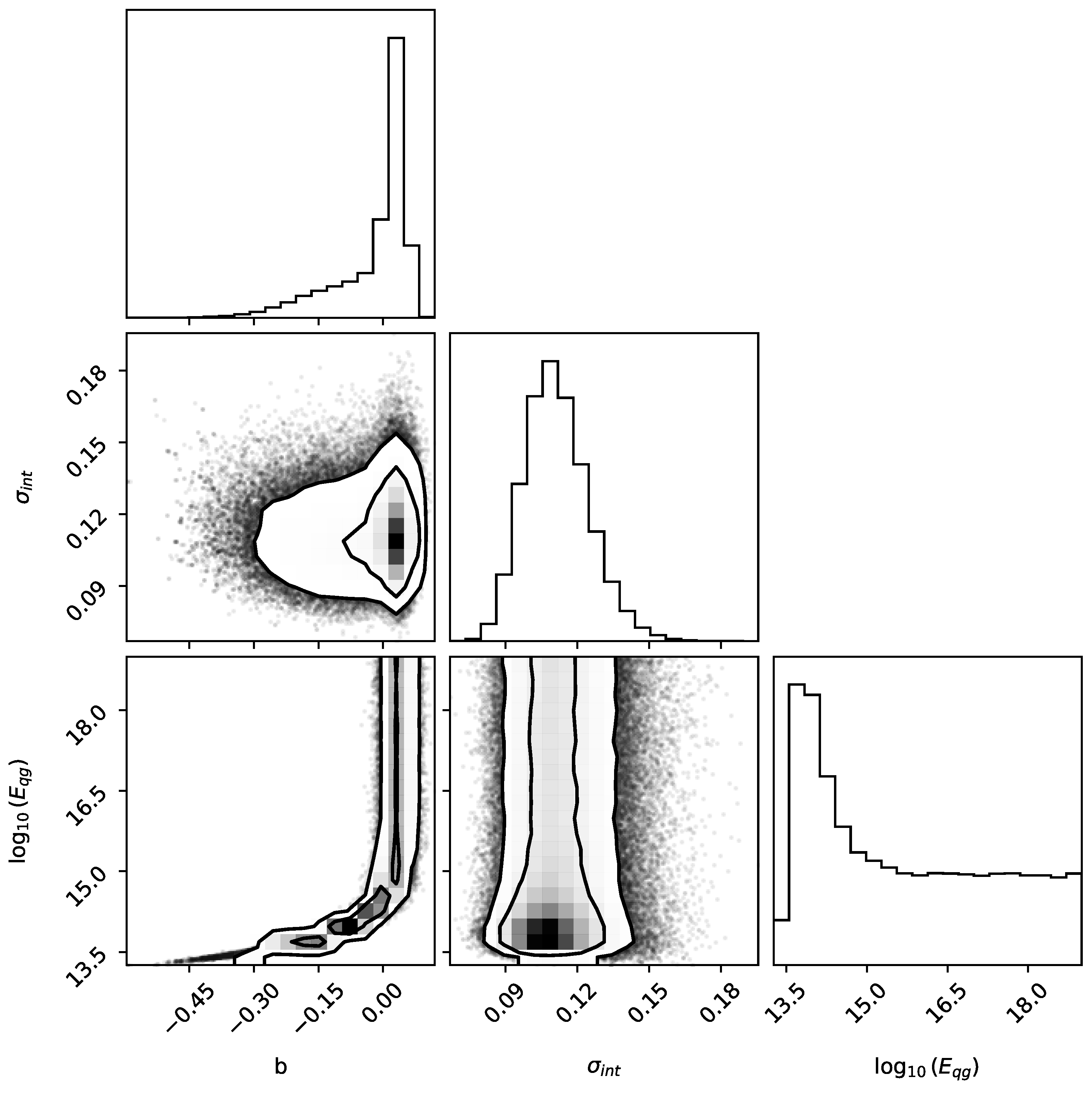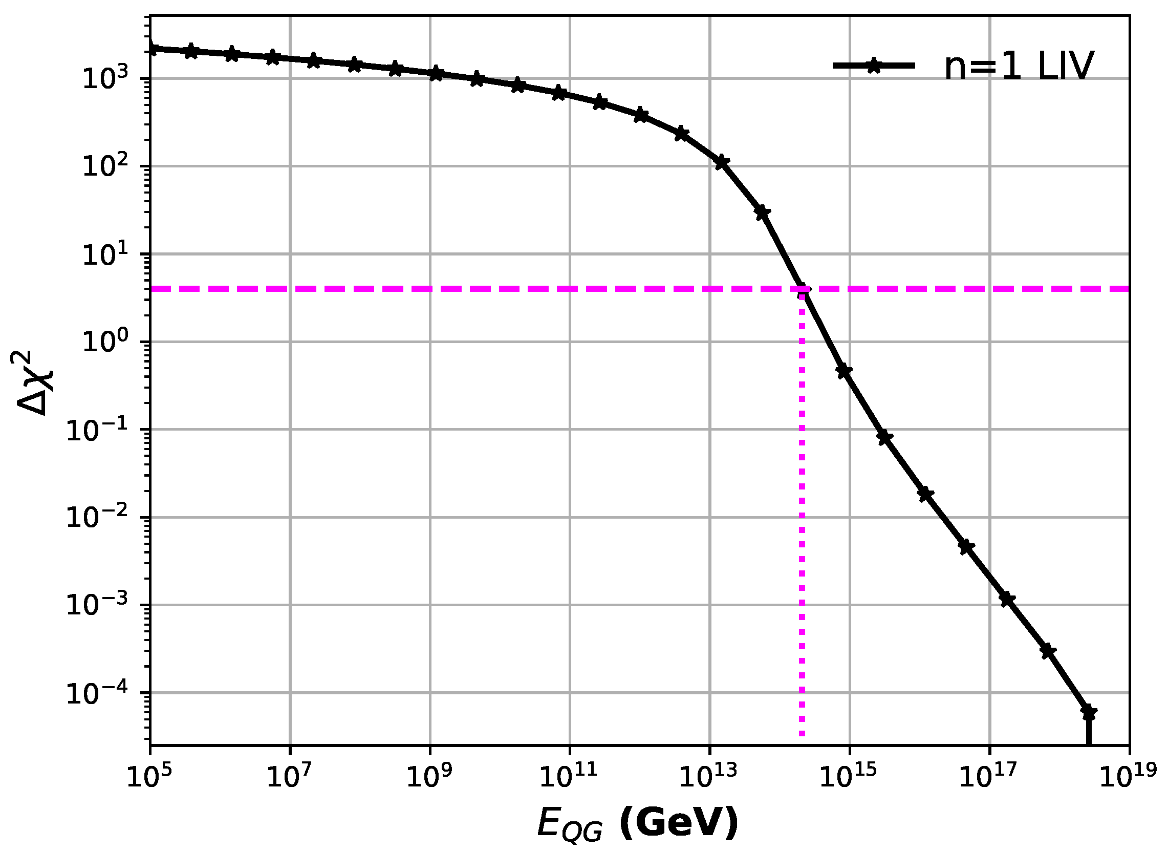In Appendix A, we compare the results of frequentist and Bayesian inference for bootstrapped version of the data where the uncertainties in the spectral lags are randomly swapped.

4. Conclusions

In this work, we have reanalyzed the data for spectral lags of 56 GRBs between two fixed energy bands in the rest frame, in order to search for LIV using frequentist inference. For this analysis, we use profile likelihood to deal with the astrophysical nuisance parameters, and we set a constraint on the energy scale of LIV for both linear and quadratic models.

We parametrize the rest-frame spectral lags as a sum of a constant intrinsic lag and LIV-induced time lag. Similarly to W17, we use a Gaussian likelihood and also incorporate another free parameter for the intrinsic scatter, which is added in quadrature to the observed uncertainties in the spectral lags. Therefore, our regression model consists of two nuisance parameters and one physically interesting parameter, viz. the energy scale for LIV.

We find that after dealing with nuisance parameters using profile likelihood, we do not find a global minimum for ${\chi }^2$ as a function of $E_{QG}$ below the Planck energy scale. These plots for $\mathrm{\Delta }{\chi }^2$ as a function of LIV for both the linear and quadratic models of LIV are shown in Figure 1 and Figure 2, respectively. Therefore, we can set one-sided lower limits at any confidence levels from the X-intercept of the $\mathrm{\Delta }{\chi }^2$ curves. These 95% confidence level lower limits obtained from $\mathrm{\Delta }{\chi }^2=4$ are given by $E_{QG}\ge 2.07\times {10}^{14}$ GeV and $E_{QG}\ge 3.71\times {10}^5$ GeV, for linear and quadratic LIV, respectively. Our lower limit for linear LIV is comparable to the value obtained in W17 ($2.2\times {10}^{14}$ GeV). The best-fit values for the two nuisance parameters evaluated at two different energies (Planck scale and 95% c.l. lower limit value) can be found in Table 1.

Therefore, we have shown that the profile likelihood method provides a viable alternative in dealing with nuisance parameters, which is complementary to the widely used Bayesian inference technique, and for our example, allows us to seamlessly infer the lower limits in an automated manner. In the spirit of open science, we have made our analysis codes publicly available, and they can be found on Github (https://github.com/vyaas3305/liv-PL-restframe, accessed on 1 March 2025).