Restrictions on Regularized Fisher and Dilatonic Spacetimes Implied by High-Frequency Quasiperiodic Oscillations Observed in Microquasars and Active Galactic Nuclei

Abstract

The Bronnikov generalization of the Fisher naked singularity and Dilatonic black hole spacetimes attracts high interest, as it combines two fundamental transitions of the solutions of Einstein equations. These are the black hole/wormhole “black bounce” transition of geometry, and the phantom/canonical transition of the scalar field, called trapped ghost scalar, combined with an electromagnetic field described by a non-linear electrodynamics. In the present paper, we put restrictions on the parameters of the Fisher (wormhole) and Dilatonic (black hole or wormhole) regularized spacetimes by using frequencies of the epicyclic orbital motion in the geodesic model for explanation of the high-frequency oscillations observed in microquasars or active galactic nuclei, where stellar mass or supermassive black holes are usually assumed.

1. Introduction

There is an increasing interest in so-called regularized spacetimes implied by a natural expectation that the effects of quantum gravity have to modify the solutions of the classical Einstein equations by substituting the spacetime singularities for some regularly behaving regions. Nevertheless, this general belief leads to significantly different results, if different approaches to quantum gravity are applied [1]. Moreover, the regularization is possible even in the framework of the general relativity, if one considers solutions of Einstein equations combined with some non-linear electrodynamics [2,3,4,5,6,7,8].

The simplest way of regularization due to the expected effects of quantum gravity was for the case of standard general relativistic black hole spacetimes, namely the singular Schwarzschild spacetime with mass parameter M, proposed by Simpson and Wiser in [9], by introducing a regularization parameter into the spherical radial coordinate r due to the relation $r\left(u\right)=\sqrt{u^2+b^2}$, where u is a new coordinate substituting r, and b is the regularization parameter. The regularized spacetime then represents a regular black hole for $b<2M$, an extremal black hole for $b=2M$, and a wormhole for $b>2M$. A regular black hole has two horizons at $u_{h\pm }=\pm \sqrt{4M^2-b^2}$; the hypersurface $u=0$, giving a minimum of the scale factor $r\left(u\right)$, represents the so-called “black bounce”, not a throat, as u is the temporal coordinate under the inner horizon $u_{h-}$1. The extremal black hole has a single horizon at $u=0$. In the wormhole case, there are no horizons of the regularized spacetime.

A widely discussed alternative to the Simpson–Visser quantum gravity regularization is represented by the black hole–white hole transition related to the loop quantum gravity models [17,18]. Here, we focus on the solutions connected to the black hole–wormhole (BH/WH) Simpson–Visser transition [9], which was generalized to the charged [19] and rotating [20,21] black hole spacetimes, including a wide range of astrophysical phenomena, as echoes in quasinormal modes, gravitational lensing, or accretion processes, studied in such spacetimes; see, e.g., refs. [22,23,24,25,26,27,28]. Of course, in the more general spacetimes, the naked singularity solutions are regularized using the Simpson–Visser method.

The crucial point of regularized spacetimes with a BH/WH transition is finding the proper stress–energy tensors composed of physical fields that could represent a relevant source of such spacetimes. Properties of the sources giving the spacetimes demonstrating the BH/WH transitions were discussed in [1,29]. It was shown that in the framework of general relativity, the sources should combine a self-interacting minimally coupled phantom scalar field and an electromagnetic field considered under non-linear electrodynamics [1]; the combination of the scalar and electromagnetic fields is necessary in order to obtain a physically relevant stress–energy tensor, but the scalar field cannot be generally a canonical field, as its phantom character is necessary to obtain the black bounce.

In [1], regularization of the singular Fisher’s solution with a massless canonical scalar field [30], corresponding to a naked singularity spacetime that is sometimes called JNW naked singularity [31], and special Dilatonic black hole solutions with interacting massless scalar and electromagnetic fields [32,33,34] has been constructed, where the scalar field has the phantom form in the strong field regime and a canonical form in the weak field regime. Detailed discussion of the character of the scalar and electromagnetic fields and the resulting stress–energy tensor can be found in [1,29].

Although the regularized Fisher and Dilatonic spacetimes have a non-standard construction because of the combination of the specific scalar and electromagnetic fields, they can be seriously considered black hole mimickers because of the extreme gravity represented by the spacetime geometry. For this reason, it is quite relevant to consider astrophysical consequences of their possible existence, and it is quite natural to confront the predictions of astrophysical processes in the corresponding backgrounds with the phenomena observed in sources where the existence of black holes is usually assumed. These are the microquasars, binary systems where stellar mass black holes are assumed [35,36,37], or active galactic nuclei (quasars), where supermassive black holes are assumed in their central part [38]. It is very important and has to be stressed that quasars can be promoted into the role of standard candles and clocks in cosmology [39,40,41]. Here, we study the spacetime geometry and its influence on the accretion Keplerian disks that can be considered uncharged, focusing attention on the epicyclic motion around stable circular geodesics representing the motion of hot spots on the Keplerian disks.

We put some fundamental restrictions on the spacetime parameters of the regularized Fisher and Dilatonic backgrounds by using the so-called geodesic model of the twin HF QPOs of X-ray radiation having fixed frequencies at a rational (usually 3:2) ratio [42,43] coming from accretion disks orbiting central objects in microquasars [37] and active galactic nuclei [38]. Of course, the HF QPO data are more abundant from the atoll sources or Z-sources where neutron stars are assumed [44,45], but the regularized Fisher and Dilatonic spacetimes cannot be considered neutron star mimickers, as they do not contain the standard nuclear matter as the source of spacetime geometry and are endowed by extremely strong magnetic fields. Therefore, we do not consider them here; furthermore, the observed HF QPOs in neutron star systems have quite different characters as they evolve with time [46].

We consider only the resulting spacetime structure of the regularized Fisher and Dilatonic backgrounds; we do not consider the influence of the related scalar and electromagnetic fields, as we focus on the behavior of uncharged matter of thin accretion disks. We study the geodesic structure of these spacetimes—we determine their circular geodesics and frequencies of the epicyclic oscillatory motion of test particles around stable circular geodesics. The frequency of the orbital motion and the related epicyclic radial and latitudinal frequencies are basic ingredients of the geodesic model of HF QPOs [42]2.

Throughout this paper, we use space-like signature $(-,+,+,+)$, and a geometric system of units in which $G=c=1$; we restore them when we need to compare our results with observational data. Greek indices run from 0–3, Latin indices from 1–3.

2. Regularized Spacetimes

Spherically symmetric regularized spacetimes describing a regularized black hole or naked singularity can be expressed in general by the line element taking in the Schwarzschild-like coordinates from the form

$$\mathrm{d}{s}^2=-f\left(x\right)\mathrm{d}{t}^2+{\displaystyle \frac{1}{f\left(x\right)}}\mathrm{d}{x}^2+r^2\left(x\right)\left(\mathrm{d}{\theta }^2+{sin}^2\theta \mathrm{d}{\phi }^2\right),$$

(1)

where x is the so-called quasiglobal radial coordinate introduced in [50]. Here, we consider two kinds of these spacetimes.

2.1. Regularized Fisher Spacetime

In 1948, I.Z. Fisher presented a static, spherically symmetric solution to Einstein’s equations in the presence of a massless scalar field [30]. This solution demonstrates how a scalar field modifies spacetime curvature and reduces to the Schwarzschild solution when the scalar field is absent. The Fisher spacetime was rediscovered by Janis, Newman, and Winicour in [31]; therefore, it is also known as the JNW naked singularity spacetime.

Fisher ordinary spacetime [30] considers the scalar mesostatic field of a point source with regard to spacetime curvature caused by this field. It was demonstrated that at a small distance from a source, the gravitational effects are so large that they cause significant changes in the behavior of the meson field. In particular, the total energy of the static field diverges logarithmically [30]. In the Fisher solution, the spacetime line element and the scalar field $\mathsf{\Phi }$ take the form [30]

$$\mathrm{d}{s}^2=-{\left(1-{\displaystyle \frac{2k}{x}}\right)}^a\mathrm{d}{t}^2+{\left(1-{\displaystyle \frac{2k}{x}}\right)}^{-a}\mathrm{d}{u}^2+x^2{\left(1-{\displaystyle \frac{2k}{x}}\right)}^{1-a}\mathrm{d}{\mathsf{\Omega }}^2,$$

(2)

$$\mathsf{\Phi }=\pm {\displaystyle \frac{{(1-a^2)}^{1/2}}{2}}ln(1-{\displaystyle \frac{2k}{x}})$$

(3)

where $k>0$ and $a\in (-1,1)$ are integration constants, such that $M=ak$ has the meaning of the gravitational Schwarzschild mass, and $C=\pm k\sqrt{1-a^2}$ is a scalar charge. As we have to consider solutions with a positive gravitational mass M, we have to restrict to values of $0<a<1$ in order to fulfil this condition under the restriction of $k>0$. In the rest of this paper, we will suppose $M=1$, i.e., $x\to x/M$, $a\to a/M$ and $k\to k/M=1/a$. The radial coordinate x in Equation (2) ranges from $2k$ to infinity, $x=2k$ corresponds to a naked singularity.

The metric regularized in the Simpson and Visser’s way demonstrates the replacement of the difference $x-2k=y$ with the expression $\sqrt{u^2+l^2}$, where u is a new radial coordinate, ranging in $u\in \mathbb{R}$, and $l>0$ is a new (Simpson–Visser) constant with the dimension of length. The Fisher metric regularized in this way then takes the form [1]

$$\mathrm{d}{s}^2=-{\left({\displaystyle \frac{y}{y+2k}}\right)}^a\mathrm{d}{t}^2+{\left({\displaystyle \frac{y}{y+2k}}\right)}^{-a}\mathrm{d}{u}^2+y^{1-a}{(y+2k)}^{1+a}d{\mathsf{\Omega }}^2,y=\sqrt{u^2+l^2},$$

(4)

being regular at all $u\in \mathbb{R}$ and asymptotically flat at $u\to \pm \infty$. The line element given by Equation (4) describes a static traversable wormhole (see the radial profile of the lapse function in Figure 1) with a Schwarzschild mass $M=ak$ at both flat asymptotics $u\to \pm \infty$ and a throat at $u=0$ with the radius

$$r_{\mathrm{th}}=l^{(1-a)/2}{(l+2k)}^{(1+a)/2}.$$

(5)

This regularized metric is not a solution of GR with a massless scalar field, but it can be related to a scalar field coupled to an electromagnetic field governed by non-linear electrodynamics, as demonstrated in [1]. We are not going into these details here, as we focus on the properties of the spacetime influencing uncharged accretion matter (test particles).

2.2. Regularized Dilatonic Spacetime

Originating from the Einstein–dilaton theory [34], the Dilatonic spacetime incorporates a dynamical scalar (dilaton) field arising in string theory. It generalizes black hole solutions and reverts to Schwarzschild or Reissner–Nordström geometry when the dilaton coupling is turned off. Dilatonic spacetimes are special solutions to the Einstein equations with a material source composed from a massless scalar field interacting with an electromagnetic field, with parameter $\lambda$ representing intensity of the coupling of the scalar and electromagnetic fields [1]. The special solution considered for the Dilatonic fields related to the string theory has the metric coefficients related to the line element given by Equation (1) determined by the expressions [33,34,51]

$$f\left(x\right)=\left(1-{\displaystyle \frac{2k}{x}}\right){\left(1+{\displaystyle \frac{p}{x}}\right)}^{-2/(1+{\lambda }^2)},r^2\left(x\right)=x^2{\left(1+{\displaystyle \frac{p}{x}}\right)}^{2/(1+{\lambda }^2)},$$

(6)

with the scalar ($\mathsf{\Phi }$) and electric ($\overrightarrow{E}$) fields given by

$$\mathsf{\Phi }=-{\displaystyle \frac{\lambda }{1+{\lambda }^2}}ln\left(1+{\displaystyle \frac{p}{x}}\right),2{\overrightarrow{E}}^2=-F_{\mu \nu }{F}^{\mu \nu }={\displaystyle \frac{Q^2}{r^4\left(x\right)}}{\mathrm{e}}^{-4\lambda \mathsf{\Phi }},$$

(7)

where $k>0$ and Q (the electric charge) are integration constants and metric parameter is their combination given by the relation

$$p=\sqrt{k^2+Q^2(1+{\lambda }^2)}-k>0.$$

(8)

Because we are concerned with the motion of uncharged matter, we are not discussing here the behavior of the related scalar and electromagnetic fields—for detailed discussion see [1].

We shall focus on the case $\lambda =1$ related to the string theory [33,34], where the line element takes the simple form

$$\mathrm{d}{s}^2=-{\displaystyle \frac{1-2k/x}{1+p/x}}\mathrm{d}{t}^2+{\displaystyle \frac{1+p/x}{1-2k/x}}\mathrm{d}{x}^2+x(x+p)\mathrm{d}{\mathsf{\Omega }}^2.$$

(9)

Then, the Schwarzschild mass $M=k+p/2=Q^2/p$, the horizon is located at $x=2k$, and a singularity is located at $x=0$. The global causal structure is the same as that of the Schwarzschild space-time. In the rest of this paper, we will suppose $M=1$, i.e., $x\to x/M$, $p\to p/M$, and $k\to k/M=1-p/2$.

Regularization of the Dilatonic spacetime is realized by replacing $dx\mapsto du$ and $x\mapsto \sqrt{u^2+l^2}$, where $l>0$ is again the regularization parameter of dimension of length. The line element can be then expressed in the form

$$\mathrm{d}{s}^2=-{\displaystyle \frac{1-2k/x}{1+p/x}}\mathrm{d}{t}^2+{\displaystyle \frac{1+p/x}{1-2k/x}}\mathrm{d}{u}^2+x(x+p)\mathrm{d}{\mathsf{\Omega }}^2,x=\sqrt{u^2+l^2}.$$

(10)

Clearly, there is $u\in \mathbb{R}$, and the regularized Dilatonic spacetime given by Equation (10) is asymptotically flat at $x\to \pm \infty$. The regular Dilatonic metric corresponds to three possible types of spacetime (see the radial profile of the lapse function illustrated in Figure 2 and Figure 3):

(i)

If $l<2k$, a regular black hole with two horizons at $u=\pm \sqrt{4k^2-l^2}$ and a black bounce at $u=0$, see Figure 3;

(ii)

If $l=2k$, a regular extremal black hole with a single extremal horizon at $u=0$ (a black throat [29]);

(iii)

If $l>2k$, a symmetric traversable wormhole with a throat at $u=0$; the throat radius is determined by the relation $r_{\mathrm{th}}=\sqrt{l(p+l)}$.

The regularized solution is related to scalar and electromagnetic fields modified in comparison to those related to the original solution—these modifications are demonstrated in [1] and will not be considered here, being irrelevant for the scope of the present paper where only motion of uncharged matter is considered.

3. Circular Geodesics in the Regularized Spacetimes

In order to test the parameters of the regularized Fisher and Dilatonic spacetimes, we study the geodesic motion of test particles in these spacetimes and find the circular geodesics of these spacetimes that govern the character of radiating accretion disks, and thus enable comparison with data obtained by observations of X-ray emission from microquasars and active galactic nuclei.

The geodesic motion in a given spacetime is determined by the metric tensor through the equations of geodesic motion

$${\displaystyle \frac{{\mathrm{d}}^2{x}^{\mu }}{\mathrm{d}{\tau }^2}}+{\mathsf{\Gamma }}_{\rho \sigma }^{\mu }{\displaystyle \frac{\mathrm{d}{x}^{\rho }}{\mathrm{d}\tau }}{\displaystyle \frac{\mathrm{d}{x}^{\sigma }}{\mathrm{d}\tau }}=0$$

(11)

that are accompanied by the norm condition for test particles having rest mass m, or for photons (or other massless particles) having $m=0$:

$$u^{\mu }{u}_{\mu }=g_{\mu \nu }{u}^{\mu }{u}^{\nu }=-\delta$$

(12)

where the parameter $\delta =m^2$.

Because of the spherical symmetry of the explored spacetimes, the geodesic motion is fixed to central planes and for simplicity, we can choose the equatorial plane at $\theta =\pi /2=const$. Due to the additional temporal and axial spacetime symmetries, two constants of the motion exist along with the fixed central plane—namely, stationarity of the spacetime implies conservation of the covariant energy E and axial symmetry implies conservation of the axial angular momentum L. It is convenient for test particles with rest mass m to introduce the specific energy and the specific axial angular momentum by the relations

$$\mathcal{E}={\displaystyle \frac{E}{m}}={\displaystyle \frac{-p_t}{m}}\mathcal{L}={\displaystyle \frac{L}{m}}={\displaystyle \frac{p_{\phi }}{m}}.$$

(13)

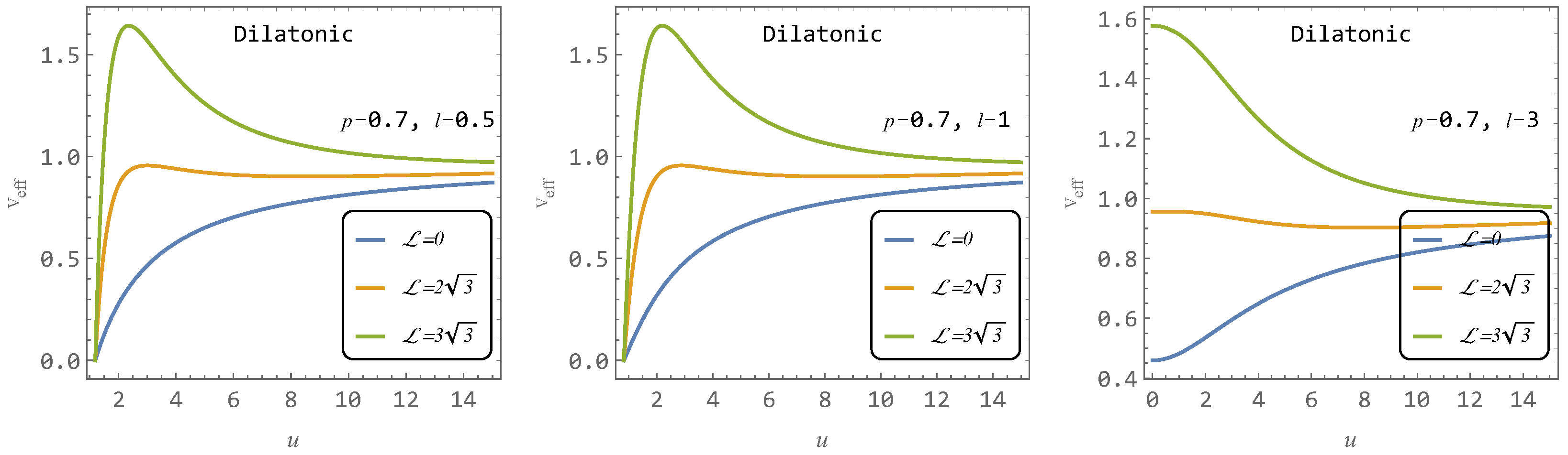
3.1. Effective Potential

In order to study the geodesic motion and to find the circular geodesics of the considered spacetimes, we use the standard method of effective potential that is given in relation to the conserved axial angular momentum of the moving particle [52]:

$$\begin{array}{c}\hfill V_{\mathrm{eff}}=f\left(r\right)\left(1+{\displaystyle \frac{{\mathcal{L}}^2}{g_{\phi \phi }}}\right)\end{array}$$

(14)

Note that for the motion of massless particles ($m=0$), the effective potential is related to the impact parameter $b=L/E$ [52]; we do not consider motion of massless particles in the present paper.

Now, we can give the effective potential explicitly for both the considered regularized spacetimes.

For the regularized Fisher spacetime, the effective potential takes the following form:

$$\begin{array}{c}\hfill V_{\mathrm{eff}}^{\mathrm{F}}={\left({\displaystyle \frac{a}{a+\frac{2}{\sqrt{l^2+u^2}}}}\right)}^a\left[{\mathcal{L}}^2{\left(l^2+u^2\right)}^{{\displaystyle \frac{a-1}{2}}}{\left(\sqrt{l^2+u^2}+2\right)}^{-a-1}+1\right]\end{array}$$

(15)

The behavior of this effective potential is characterized in Figure 4. Notice that the effective potential is decreasing with increasing parameter l.

For the regularized Dilatonic spacetimes, the effective potential takes the following form:

$$\begin{array}{c}\hfill V_{\mathrm{eff}}^{\mathrm{D}}={\displaystyle \frac{\left(x+p-2\right)\left(px+l^2+{\mathcal{L}}^2+l^2\right)}{x{\left(x+p\right)}^2}}\end{array}$$

(16)

The behavior of this effective potential is characterized in Figure 5. Notice that the effective potential is decreasing with increasing parameter l.

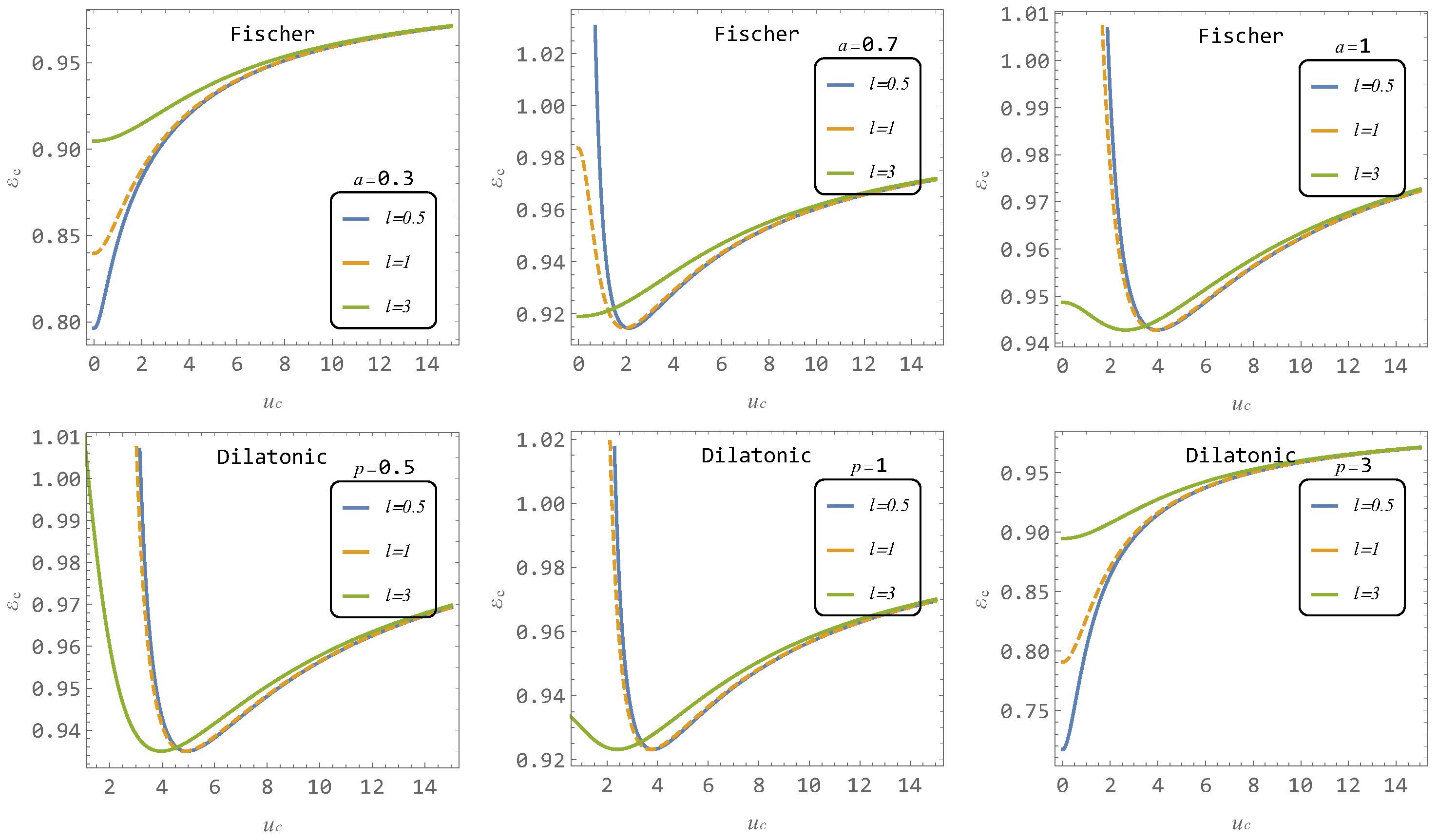
3.2. Circular Geodesics

The circular geodesics are determined by local extrema of the effective potential implied by the condition

$${\displaystyle \frac{\mathrm{d}{V}_{\mathrm{eff}}}{\mathrm{d}u}}=0.$$

(17)

Using this general condition, we can find the radial profiles of the particle (quadratic) specific axial angular momentum in both the considered regularized spacetimes in the following form:

$$\begin{array}{cc}\hfill & {\mathcal{L}}_{\mathrm{c}\left(\mathrm{F}\right)}^2(u,l,a)=-{\displaystyle \frac{a\left[\left(y+4\right)y^2+4y\right]y^{-a}{\left(y+2\right)}^a}{a^{2}y-a{y}^2+2\left(y+1\right)}},\hfill \\ \hfill & {\mathcal{L}}_{\mathrm{c}\left(\mathrm{D}\right)}^2(u,l,p)={\displaystyle \frac{2x^2\left(x+p\right)}{p\left(3x-2\right)-6x+p^2+2x^2}}.\hfill \end{array}$$

(18)

These radial profiles are illustrated in Figure 6. Notice that the radial profiles in the Fisher spacetimes depend on the spacetime parameters weakly in comparison with the radial profiles in the Dilatonic spacetimes, demonstrating significantly stronger variability.

The covariant specific energy of a particle following the circular geodesics is determined by the value of the effective potential at the extremal point, given by specific axial angular momentum.The radial profiles of ${\mathcal{E}}^2$ are given for the regularized Fisher and Dilatonic spacetimes by the relations

$$\begin{array}{cc}\hfill & {\mathcal{E}}_{c\left(F\right)}^2(u,l,a)={\displaystyle \frac{{\left(1-\frac{2}{ay}\right)}^a}{y\left(y+2\right)\left[a^{2}y-a{y}^2+2\left(y+1\right)\right]}}\times \hfill \\ \hfill & \{l^2\left[a^2\left(y+2\right)-a\left(3y+2u^2+4\right)+2\left(y+3\right)\right]-a{u}^4-a{l}^4+\hfill \\ \hfill & u^2\left[a^2\left(y+2\right)-a\left(3y+4\right)+2\left(y+3\right)\right]-4(a-1)y\},\hfill \\ \hfill & {\mathcal{E}}_{c\left(D\right)}^2(u,l,p)={\displaystyle \frac{\left(x+p-2\right)\left[(p-2)x+x^2\right]\left(3px+p^2+2x^2\right)}{x{\left(x+p\right)}^2\left[p\left(3x+p-2\right)-6x+2x^2\right]}}.\hfill \end{array}$$

(19)

The radial profiles of the covariant specific energy are illustrated in Figure 7 and demonstrate similar differences as in the case of radial profiles of the specific angular momentum.

3.2.1. Regions of Existence

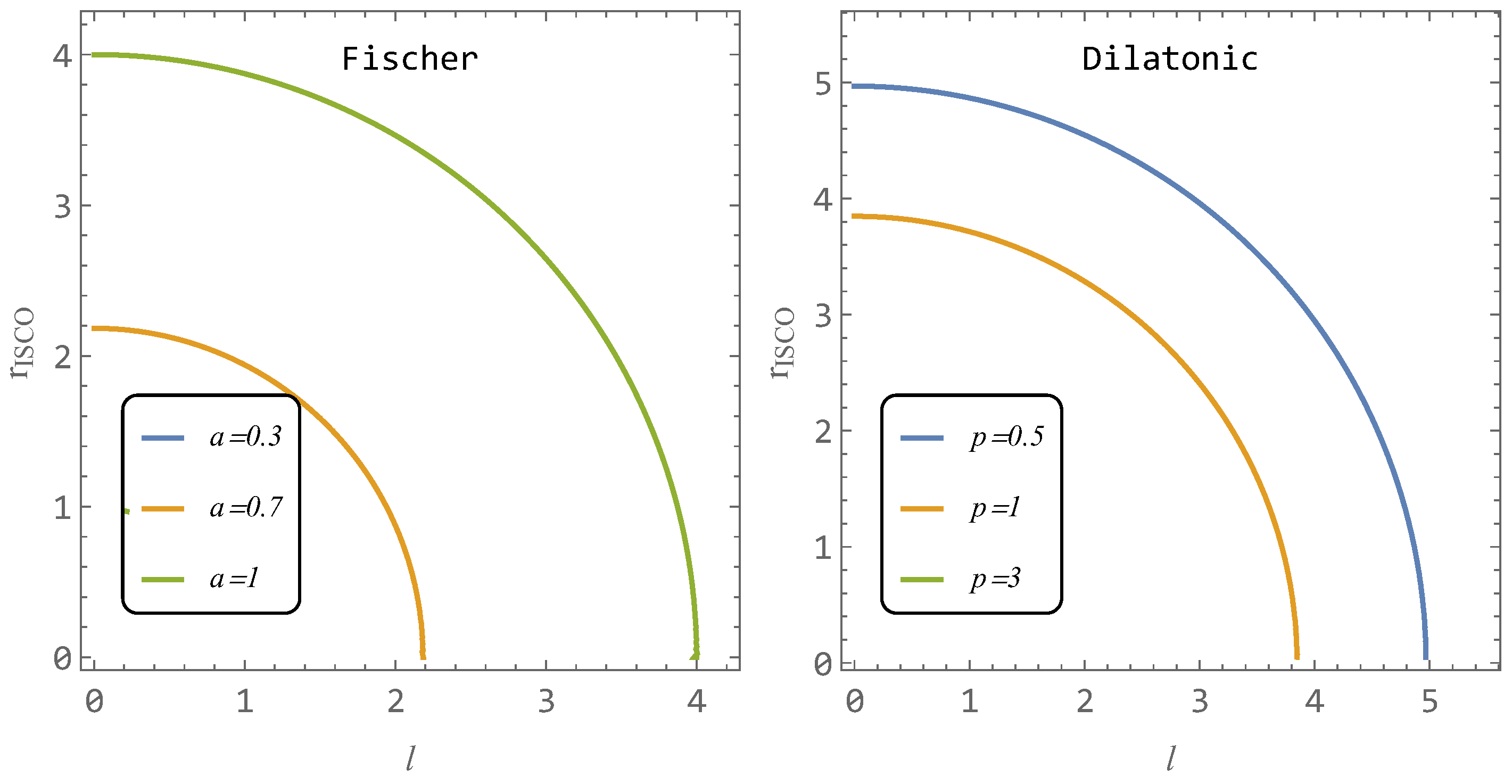
The regions allowing for the existence of circular geodesics are characterized in Figure 8 and Figure 9. We can see that in the regularized Fisher spacetimes, the circular orbits can exist at all allowed radii if the parameter $a<0.5$, while a circular null geodesic exists for $a>0.5$—it is reaching maximal radius at $u_{\mathrm{cng}}=1$ for the limiting value $a=1$ and $l=0$; for increasing l and fixed a, the radius of the circular null geodesic is decreasing to $u_{\mathrm{cng}}=0$ at $l=1$. The circular geodesic exists at all $u>0$ for $l>1$ (and $a=1$). We can thus see that the special annular region where no circular geodesic exists, being surrounded by these orbits, observed in the original Fisher naked singularity spacetimes [53,54], similarly to the case of the Kehagias–Sfetsos naked singularity spacetimes of the Horava gravity [55], are not present due to the regularization procedure. In the Dilatonic spacetimes, the circular null geodesics exist for $p<2$. There is $u_{\mathrm{cng}}=3$ for $p=0$ and $l=0$ (corresponding to the Schwarzschild geometry), while with fixed $p=0$, it is reaching $u_{\mathrm{cng}}=0$ for $l=3$. For $p=2$, we have the limiting value of $u_{\mathrm{cng}}=0$ obtained for $p=2$ and $l=0$. For $p>2$, the circular geodesic exists at all $u>0$. Again, there is no annular region forbidding the existence of circular geodesics in regularized Dilatonic spacetimes. Note that the circular null geodesics do not correspond to the photon spheres because of the existence of non-linear electromagnetic fields in the regularized spacetimes [47,48,49].

3.2.2. ISCO

The marginally stable (innermost) circular geodesics (ISCOs) of the considered regularized Fisher and Dilatonic spacetimes are determined by the condition

$${\left.{\displaystyle \frac{{\mathrm{d}}^2{V}_{\mathrm{eff}}\left(r\right)}{\mathrm{d}{r}^2}}\right|}_{r=r_{\mathrm{c}}}=0.$$

(20)

This condition is related to the circular orbits. For the regularized Fisher spacetimes, the condition takes the form

$$\begin{array}{ccc}& & {\left(1-{\displaystyle \frac{2}{ay}}\right)}^a\hfill \\ \hfill \times & {\displaystyle \{}& -32(-1+a)y+a{l}^6\left[-6+a(2-4a+y)\right]\hfill \\ & +& a{u}^6\left[-6+a(2-4a+y)\right]+l^2\{80+88y+8u^2(11+2y)\hfill \\ & +& 4a^4\left[2y+u^2(4+y)\right]-2a\left[8(5+4y)+u^2(44+9u^2+26y)\right]\hfill \\ & +& a^2\left[16+64y+u^2\left(88+16y+3u^2(2+y)\right)\right]-4a^3\left[4(1+y)+u^2(10+3u^2+8y)\right]\}\hfill \\ & +& l^4\{44+8y+a[-2(22+9u^2+13y)\hfill \\ & +& a\left(44+8y+3u^2(2+y)+2a^2(4+y)-4a(5+3u^2+4y)\right)\left]\right\}\hfill \\ & +& 2u^4\left\{22+4y+a\left[-22-13y+a\left(22+4y+a(-10+4a-8y+ay)\right)\right]\right\}\hfill \\ & +& 8u^2\left\{10+11y+a\left[-2(5+4y)+a\left(2+8y+a(-2-2y+ay)\right)\right]\right\}{\displaystyle \}}=0.\hfill \end{array}$$

(21)

For the regularized Dilatonic spacetime, we arrive to the form

$$\begin{array}{cc}& l^4+p^4+u^4-6u^{2}x+p^2\left(6u^2-8x\right)+4p{u}^2\left(x-3\right)+\\ & p^3\left(4x-2\right)+2l^2\left[3\left(p-2\right)p+u^2-3x+2px\right]=0.\end{array}$$

(22)

Results of numerical calculations giving the ISCO radius are illustrated for characteristic values of the spacetime parameters in Figure 10.

From our analysis, it follows that the position of the ISCO in the Fisher spacetime and the Dilatonic spacetime disappears for certain combinations of the parameters l and a (p). This is because stable circular orbits can exist at any radius, and there is no limitation on their existence. For Fisher spacetime, the ISCO ceases to exist approximately for $a\lesssim 0.5$. On the other hand, for Dilatonic spacetime, the ISCO disappears for values greater than approximately $p\gtrsim 2$. This is evident from Figure 6 and Figure 7, where no minima of $\mathcal{L}$ and $\mathcal{E}$ exist for relevant values of the spacetime parameters.

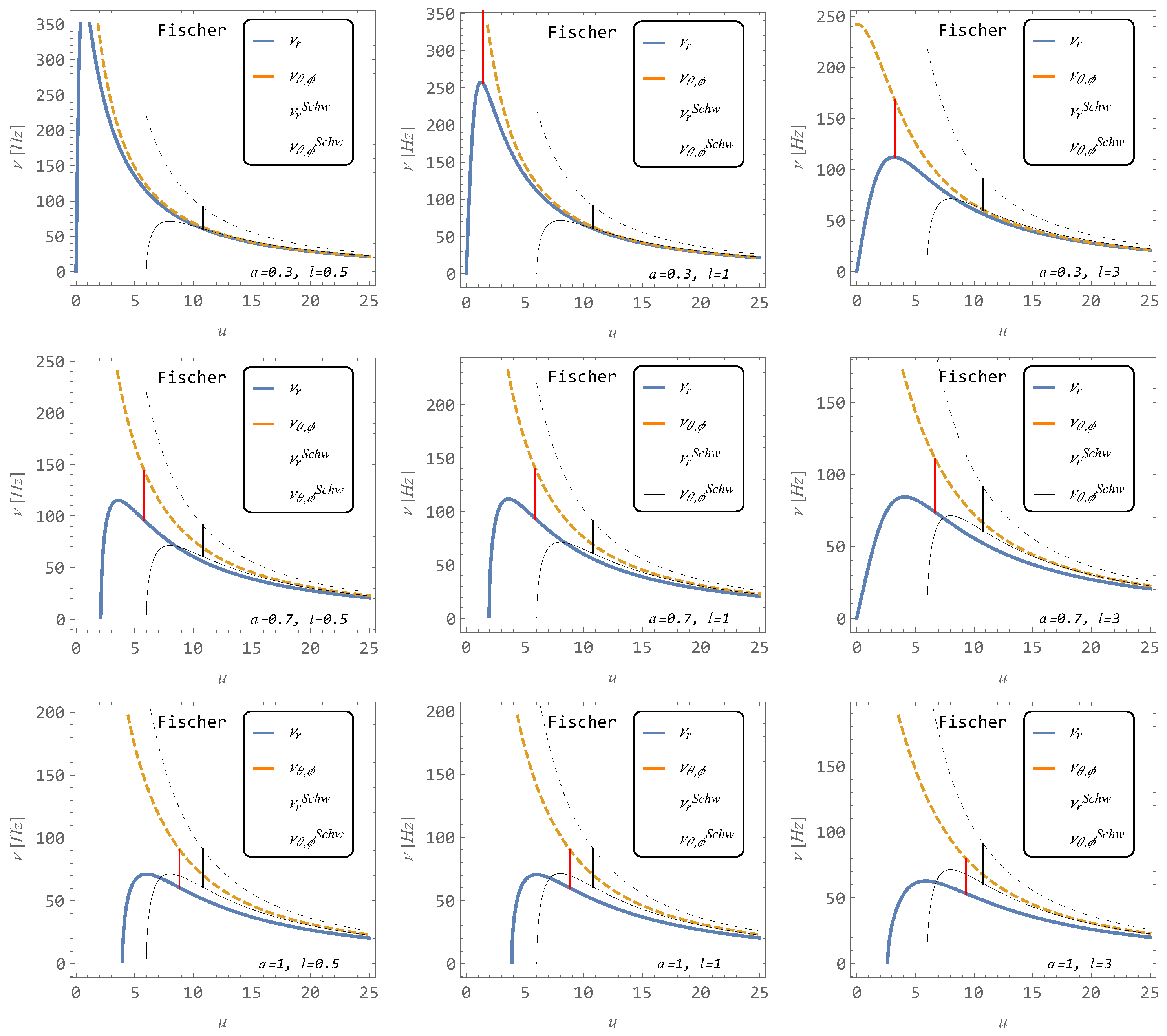
4. Epicyclic Oscillations Around Stable Circular Geodesics of the Regularized Spacetimes

In the linear perturbation regime, the radial ($\delta u\left(\tau \right)$) and latitudinal ($\delta \theta \left(\tau \right)$) epicyclic motion around stable circular orbits is governed by the equation of the harmonic oscillator [42]

$$\begin{array}{c}\hfill \delta \ddot{u}+{\overline{\omega }}_r^2\delta u=0,\delta \ddot{\theta }+{\overline{\omega }}_{\theta }^2\delta \theta =0,\end{array}$$

(23)

where $\overline{{\omega }_r}$ ($\overline{{\omega }_{\theta }}$) represents the angular velocity of the radial (latitudinal or vertical) epicyclic oscillations as measured at the proper time $\tau$ of the oscillating particle. These angular frequencies are determined by the Hamiltonian separated into its dynamic and potential parts [56]

$$\begin{array}{c}\hfill H=H_{\mathrm{dyn}}+H_{\mathrm{pot}},\end{array}$$

(24)

where

$$\begin{array}{cc}\hfill H_{\mathrm{dyn}}& ={\displaystyle \frac{1}{2}}\left(g^{uu}{p}_u^2+g^{\theta \theta }{p}_{\theta }^2\right),\end{array}$$

(25)

$$\begin{array}{cc}\hfill H_{\mathrm{pot}}& ={\displaystyle \frac{1}{2}}\left(g^{tt}{E}^2+g^{\phi \phi }{L}^2+m^2\right),\end{array}$$

(26)

and are given by the relations

$$\begin{array}{ccc}\hfill {\overline{\omega }}_r^2& =& {\displaystyle \frac{1}{g_{rr}}}{\displaystyle \frac{{\partial }^2{H}_{\mathrm{pot}}}{\partial r^2}},\hfill \\ \hfill {\overline{\omega }}_{\theta }^2& =& {\displaystyle \frac{1}{g_{\theta \theta }}}{\displaystyle \frac{{\partial }^2{H}_{\mathrm{pot}}}{\partial {\theta }^2}}.\hfill \end{array}$$

(27)

The derivations are calculated by using relations for energy $E=E_c$ and axial angular momentum $L=L_c$ at the positions of the stable circular orbits.

The orbital angular frequency of the circular motion is determined by the relation

$${\overline{\omega }}_{\phi }={\displaystyle \frac{\mathcal{L}}{g_{\theta \theta }}}.$$

(28)

Equation (27) gives angular frequencies as measured by a local observer related to the oscillating particle, but we have to find the angular frequencies as measured by static observers at infinity who represent real observers observing the oscillations from a large distance. Therefore, we rescale the locally measured angular frequencies by a corresponding redshift factor related to the orbital motion along the stable circular geodesic at $r_c$ and find

$$\begin{array}{c}\hfill \omega ={\displaystyle \frac{\overline{\omega }}{-g^{tt}\mathcal{E}}}.\end{array}$$

(29)

In order to obtain the observed frequencies in the standard units, we have to use the transformation

$$\begin{array}{c}\hfill \nu ={\displaystyle \frac{1}{2\pi }}{\displaystyle \frac{c^3}{GM}}{\displaystyle \frac{\overline{\omega }}{-g^{tt}\mathcal{E}}},\end{array}$$

(30)

giving expressions that could be directly used in fitting to observational data.

Using relations (4) and (10), (18), and (26) in Equation (27), we arrive at the formulas for the epicyclic frequencies measured in regularized Fisher spacetimes in the form

$$\begin{array}{cc}\hfill & {\overline{\omega }}_{\theta }={\overline{\omega }}_{\phi }=\sqrt{{\displaystyle \frac{a\left(2y+y^2\right)y^{\frac{a}{2}-1}{\left(y+2\right)}^{-a-2}}{y-2a+1}}},\hfill \end{array}$$

(31)

$$\begin{array}{cc}\hfill & {\overline{\omega }}_r^2={\displaystyle \frac{a{u}^2{\left(\frac{y}{y+2}\right)}^a}{y^2{(y+2)}^4(-2a+y+1)}}\times \hfill \\ \hfill & \left\{l^4+2l^2\left(u^2+3y+7\right)+4a^2\left(y^2+4y+4\right)-6a\left[(y+5)y^2+8y+4\right]+\right.\hfill \\ \hfill & \left.u^4+6u^{2}y+14u^2+16y+8\right\},\hfill \end{array}$$

(32)

where $y=\sqrt{u^2+l^2}$, as defined in Equation (4). In the case of the regularized Dilatonic spacetime, we arrive at the formulas

$$\begin{array}{cc}\hfill & {\overline{\omega }}_{\theta }={\overline{\omega }}_{\phi }={\displaystyle \frac{\sqrt{p+2}}{\sqrt{2}{\left[p\left(x^2-4x\right)+x^2\left(x-3\right)-p^2\right]}^{1/2}}},\hfill \end{array}$$

(33)

$$\begin{array}{cc}\hfill & {\overline{\omega }}_r^2={\displaystyle \frac{u^2(p+2)}{2x^3\left(x-2\right){\left(p+x\right)}^4\left[p\left(x^2-4x\right)+x^3-3x^2-p^2\right]}}\times \hfill \\ \hfill & \left\{-2p^4\left(x-2\right)+10p^3\left(2x-x^2\right)+p^2{x}^2\left(x^2-22x+40\right)+\right.\hfill \\ \hfill & \left.2p{x}^2\left[l^2\left(x-11\right)+u^2\left(x-11\right)+18x\right]+x^4\left(x^2-8x+12\right)\right\}.\hfill \end{array}$$

(34)

where $x=\sqrt{u^2+l^2}$, as defined in Equation (10).

The resulting radial profiles of the observed radial and latitudinal (orbital) frequencies are presented in Figure 11 and Figure 12. As is usual for the spherically symmetric spacetimes, the angular frequency of the latitudinal epicyclic oscillations equals the angular frequency of the orbital motion.

Since the twin HF QPOs observed in microquasars and active galactic nuclei are mainly detected with the frequency ratio very close to 3:2, we show in the presented radial profiles the radius of the spacetime where the ratio of the frequencies of the radial and vertical (latitudinal) epicyclic oscillations takes the ratio 3:2, denoted as $u_{3:2\left(F\right)}$ or $u_{3:2\left(D\right)}$ for the regularized Fisher or Dilatonic spacetimes, and compare this radius with the radius corresponding to the frequency ratio 3:2 for oscillations in the Schwarzschild spacetime.

Because of astrophysical relevance of the radius where the frequency ratio 3:2 occurs, we demonstrate dependence of the position of the radii with frequency ratio 3:2 on the spacetime parameters of the considered spacetimes in Figure 13.

We can see that with increasing parameter l, the frequency radius $u_{3:2}$, where ratio ${\nu }_{\mathrm{U}}$:${\nu }_{\mathrm{L}}=$ 3:2 occurs, is increasing. For $l>40$, the radius $u_{3:2}>40M$ for both spacetimes is seen in Figure 13.

5. Restrictions on the Regularized Spacetime Parameters Due to Fits to the HF QPOs Observed in Microquasars and Active Galactic Nuclei

In this section, we compare astrophysical data coming from X-ray observations of twin HF QPOs in some microquasars and active galactic nuclei with the geodesic model of twin HF QPOs applied to the regularized Fisher and Dilatonic spacetimes. The comparison with the twin HF QPO data enables us to obtain restrictions on the parameters of the spacetimes under consideration, which are well founded by observations.

5.1. Geodesic Model of HF QPOs

In some microquasars, we observe twin HF QPOs in the X-radiation coming from their accretion disks [37,57,58]. The frequency ratio of the twin (“upper” and “lower”) oscillations is observed with the small number ratios 3:2, 2:1, 4:3, 3:1, etc. However, a large majority of the twin HF QPOs observed in microquasars is in the frequency ratio 3:2 [37,59]. Twin HF QPOs demonstrating the same frequency ratio are observed also in some active galactic nuclei [38]. Magnitudes of the observed frequencies correspond to frequencies of the orbital motion of accreted uncharged matter in close vicinity of the black hole considered in the center of the accretion disk in both microquasars, where stellar mass black holes are assumed, and in active galactic nuclei, where supermassive black holes are assumed. Therefore, the community of astrophysicists accepts as realistic the geodesic model of HF QPOs assuming the observed frequencies related to proper combinations of the orbital frequency of the circular geodesic motion and the frequencies related to the epicyclic oscillatory motion around stable circular geodesics [27,42,60,61].

The relativistic precession variant of the geodesic model [62] assumes a blob of a thin accretion disk orbiting the black hole and identifies the observed HF QPO frequencies ${\nu }_u,{\nu }_l$, with a combination of the orbital and epicyclic frequencies given by the relations

$$\begin{array}{c}\hfill {\nu }_u={\nu }_{\varphi },\\ \hfill {\nu }_l={\nu }_{\varphi }-{\nu }_r.\end{array}$$

(35)

Other variants of the geodesic model, inspired by the Rezzolla model [63], assume oscillations of a torus. If the torus is slender, then the frequencies of the torus oscillations are equal to the frequencies of the epicyclic oscillation in the torus center [61,64]3.

However, the twin HF QPOs observed in microquasars demonstrate strong stability, i.e., in different observations they appear or reappear with the same magnitudes [37,57]. As in the geodesic model, the frequencies depend on the position of the oscillating hot spot or the slender torus, we have to find a reason why the position related to the fixed observed frequencies is the relevant one. A natural idea of this kind was proposed by Abramowicz and Kluzniak and is related to the resonance phenomena [60,75,76,77]. The resonance variant of the geodesic model assumes in its simplest form a non-linear resonance of the radial and vertical oscillations of a slender torus, with frequencies related to the twin HF QPOs in the elementary form

$$\begin{array}{c}\hfill {\nu }_u={\nu }_{\theta },\\ \hfill {\nu }_l={\nu }_r.\end{array}$$

(36)

For more complex resonance variants of the geodesic model, see [61], and for more complex treatment of the resonant phenomena, see [42]. Furthermore, if a parametric resonance is relevant, the 3:2 resonance is the strongest one [78].

For the above-mentioned reasons, the resonance variant of the geodesic model is widely used for fitting the observational data from microquasars or active galactic nuclei [79,80] to test various models of black holes, naked singularities, or wormholes, constructed under various alternative models of gravity, or in GR combined with non-linear electrodynamics, or for black holes or other central objects in various surroundings or under various influences.

Here, we apply the simplest resonance variant of the geodesic model in fitting data from both microquasars and active galactic nuclei in order to restrict the parameters of the regularized Fisher and Dilatonic spacetimes.

5.2. Comparison of Observational Data from Microquasars with the Geodesic Model of Twin HF QPOs Applied for the Regularized Spacetimes

Here, we focus on fitting the twin HF QPO data observed in microquasars. The astrophysical data are taken from the following three sources: GRG 1915-105, XTE 1530-564, and GRO1655-40, presented in

Table 1. Observed twin HF QPO data for the three microquasars, and the restrictions on mass of their central object.

Source	${\mathit{\nu }}_{\mathit{U}}$ [Hz]	${\mathit{\nu }}_{\mathit{L}}$ [Hz]	$\mathit{M}/{\mathit{M}}_{\odot }$
GRO 1655-40	447–453	295–305	6.03–6.57
XTE 1550-564	273–279	179–189	8.5–9.7
GRS 1915+105	165–171	108–118	9.6–18.4

[37,81].

It should be noticed that sole twin peaks with exact ratio 3:2 are surely present only at GRO 1655-40 microquasar, but some doubts on their presence in XTE 1550-564 are given in [35]. More complex varieties of frequencies and their ratios are observed in the case of the GRS 1915+105 source—modified estimates of the mass of the central object in this source are mentioned in [82].

The possible fits are shown in Figure 14, which illustrates the fits for the regularized Fisher wormhole spacetimes (left), and separately the fits for the Dilatonic spacetimes describing both black holes and wormholes (right) by using the profile of the upper frequency given by the resonant variant of the geodesic model.

It is evident that for both the regularized Fisher wormhole spacetimes and Dilatonic black hole or wormhole spacetimes, we can always find a combination of the spacetime parameters that enables fitting the data from the three microquasars.

The constraints on the parameters of the regularized Fisher and Dilatonic spacetimes following from the fitting procedure related to the resonance variant of the geodesic model of HF QPOs are determined by the condition that at least one of the microquasar data are met by the curve corresponding to the applied variant of the geodesic model by fitting the selected three microquasar data. The constraints are given by the shaded region displayed in Figure 15. We can see that in both spacetimes, the range of allowed values of the regularization parameter is restricted to $l<3$. In the case of Dilatonic spacetime, the wormhole case is the proper one for the fitting.

5.3. Comparison of Observational Data from Active Galactic Nuclei with the Geodesic Model of HF QPOs Model Applied to the Regularized Spacetimes

In this section, we focus on the observational HF QPO data from active galactic nuclei where usually a supermassive black hole is assumed. We use the upper observed frequency again, and for clarity divide the sources into two sets.The list of these datasets is provided in

Table 2. Observations of QPOs around supermassive BHs [38].

Number	Name	BH Spin	log ${\mathit{M}}_{\mathbf{BH}}$ (${\mathit{M}}_{\odot }$)	${\mathit{f}}_{\mathbf{UP}}$ (Hz)
1	RE J1034+396	0.998	$6.0_{-3.49}^{+1.0}$	$2.7\times {10}^{-4}$
2	1H0707-495	>0.976	$6.{36}_{-0.06}^{+0.24}$	$2.6\times {10}^{-4}$
3	MCG-06-30-15	>0.917	$6.{20}_{-0.12}^{+0.09}$	$2.73\times {10}^{-4}$
4	Mrk 766	>0.92	$6.{82}_{-0.06}^{+0.05}$	$1.55\times {10}^{-4}$
5	ESO 113-G010	0.998	$6.{85}_{-0.24}^{+0.15}$	$1.24\times {10}^{-4}$
6	ESO 113-G010b	0.998	$6.{85}_{-0.24}^{+0.15}$	$6.79\times {10}^{-5}$
7	1H0419-577	>0.98	$8.{11}_{-0.50}^{+0.50}$	$2.0\times {10}^{-6}$
8	ASASSN-14li	>0.7	$6.{23}_{-0.35}^{+0.35}$	$7.7\times {10}^{-3}$
-	TON S 180	<0.4	$6.{85}_{-0.5}^{+0.5}$	$5.56\times {10}^{-6}$
-	RXJ 0437.4-4711	-	$7.{77}_{-0.5}^{+0.5}$	$1.27\times {10}^{-5}$
-	XMMU J134736.6+173403	-	$6.{99}_{-0.20}^{+0.46}$	$1.16\times {10}^{-5}$
-	MS 2254.9-3712	-	$6.6_{-0.60}^{+0.39}$	$1.5\times {10}^{-4}$
-	Sw J164449.3+573451	-	$7.0_{-0.35}^{+0.30}$	$5.01\times {10}^{-3}$

[38].

The resulting fits (and parameters fitting at least one source) are shown in Figure 16, Figure 17, Figure 18 and Figure 19, respectively. It is clear that both the regularized Fisher and Dilatonic spacetimes are capable of fitting all sources, with an appropriate choice of parameters, except the “island” source Sw J164449.3+573451. Note that this special source is not available in other attempts for the fitting; see, e.g., ref. [74].

6. Discussion

Our study of the two spacetimes (Fisher, of naked singularity type, and Dilatonic of black hole/naked singularity type), where regularization of the Simpson–Vissertype implies the necessity of a specific combination of the scalar and electromagnetic fields and transformation of these spacetime into the wormhole type (Fisher) or black bounce type (Dilatonic) that can serve as black hole mimickers, was concentrated onto the epicyclic motion around circular geodesics, and its application for explanation of twin HF QPOs observed in microquasars and active galactic nuclei focuses on the case of the frequency ratio 3:2.

Surprisingly, we have found that the radial profiles of the epicyclic frequencies in both the considered spacetimes generally have the same character as in the standard Schwarzschild spacetime, but the significant shift of the position of possible resonant phenomena with the frequency ratio 3:2 is observed. This shift, corresponding to the increase of the magnitude of frequencies that are in the 3:2 ratio in correspondence with those related to the Schwarzschild black holes having the same mass, is observed in both the spacetimes, and is more significant in the wormhole spacetimes. This effect is reflected in the fitting procedure by the resonance variant of the geodesic model of HF QPOs, having a positive role especially in the case of fitting the sources in active galactic nuclei.

The regularized Fisher and Dilatonic spacetimes demonstrate greater flexibility, accommodating ASASSN-14li within specific parameter ranges. The fitting by the regularized Fisher spacetimes is particularly effective only for small range values about $a\sim 0.35$ and $l\sim 0.5$. In the case of regularized Dilatonic spacetimes, one can fit the same source by lower values of the parameter l (approximately $l\sim$ 0.3–1) and moderate values of p (around $p\sim$ 2–3) in the wormhole regime.

As shown in Figure 17 and Figure 19, the data points within the shaded area (these correspond to the cases where the fit is possible at least for one of the selected sources) demonstrate a high level of agreement of the theoretical predictions given by the resonance variant of the geodesic model of HF QPOs, and the related assembly of observed astrophysical data coming from the considered sources.

7. Conclusions

We have studied the circular orbits and related epicyclic oscillatory motion around stable circular geodesics in order to obtain some restrictions on the parameters of the regularized Fisher and Dilatonic spacetimes by fitting the twin HF QPO observational data coming from the three standard microquasars and a selection of the active galactic nuclei. By using the most common resonant variant of the geodesic model of the twin HF QPOs, we have found that the restriction on the spacetime parameters of the considered spacetimes is much more strict in the case of the microquasars, where only the wormhole spacetimes are selected as allowable. On the other hand, in the case of the data coming from the active galactic nuclei, a much more extended range of allowed values of the spacetime parameters has been found. Note that for microquasars, the regularized Fisher and Dilatonic spacetime (more specifically, the Dilatonic wormhole spacetimes) provides successful fits for all sources. For supermassive black holes, both the Fisher and Dilatonic spacetime fits all sources except SwJ (island source). Of course, it would be interesting to compare our results related to the simplest model based on the purely geodesic motion with optical phenomena where the influence of electromagnetic field is reflected in the effective geometry governing the photon motion [47,48,49]. We plan such a study in a forthcoming paper.

References

1. Bronnikov, K.A. Black bounces, wormholes, and partly phantom scalar fields. Phys. Rev. D 2022, 106, 064029. [Google Scholar] [CrossRef]
2. Born, M. On the Quantum Theory of the Electromagnetic Field. Proc. R. Soc. Lond. Ser. A 1934, 143, 410–437. [Google Scholar] [CrossRef]
3. Born, M.; Infeld, L. Foundations of the New Field Theory. Proc. R. Soc. Lond. Ser. A 1934, 144, 425–451. [Google Scholar] [CrossRef]
4. Bronnikov, K.A. Regular magnetic black holes and monopoles from nonlinear electrodynamics. Phys. Rev. D 2001, 63, 044005. [Google Scholar] [CrossRef]
5. Bronnikov, K.A. Nonlinear electrodynamics, regular black holes and wormholes. Int. J. Mod. Phys. D 2018, 27, 1841005. [Google Scholar] [CrossRef]
6. Fan, Z.Y.; Wang, X. Construction of regular black holes in general relativity. Phys. Rev. D 2016, 94, 124027. [Google Scholar] [CrossRef]
7. Toshmatov, B.; Stuchlík, Z.; Ahmedov, B. Comment on “Construction of regular black holes in general relativity”. Phys. Rev. D 2018, 98, 028501. [Google Scholar] [CrossRef]
8. Kruglov, S.I. Universe acceleration and nonlinear electrodynamics. Phys. Rev. D 2015, 92, 123523. [Google Scholar] [CrossRef]
9. Simpson, A.; Visser, M. Black-bounce to traversable wormhole. J. Cosmol. Astropart. Phys. 2019, 2019, 042. [Google Scholar] [CrossRef]
10. Bronnikov, K.A.; Fabris, J.C. Regular Phantom Black Holes. Phys. Rev. Lett. 2006, 96, 251101. [Google Scholar] [CrossRef]
11. Bronnikov, K.A.; Dehnen, H.; Melnikov, V.N. Regular black holes and black universes. Gen. Relativ. Gravit. 2007, 39, 973–987. [Google Scholar] [CrossRef]
12. Bolokhov, S.V.; Bronnikov, K.A.; Skvortsova, M.V. Magnetic black universes and wormholes with a phantom scalar. Class. Quantum Gravity 2012, 29, 245006. [Google Scholar] [CrossRef]
13. Clément, G.; Fabris, J.C.; Rodrigues, M.E. Phantom black holes in Einstein-Maxwell-dilaton theory. Phys. Rev. D 2009, 79, 064021. [Google Scholar] [CrossRef]
14. Azreg-Aïnou, M.; Clément, G.; Fabris, J.C.; Rodrigues, M.E. Phantom black holes and sigma models. Phys. Rev. D 2011, 83, 124001. [Google Scholar] [CrossRef]
15. Bronnikov, K. Scalar Fields as Sources for Wormholes and Regular Black Holes. Particles 2018, 1, 5. [Google Scholar] [CrossRef]
16. Nishonov, I.; Zahid, M.; Khan, S.U.; Rayimbaev, J.; Abdujabbarov, A. Dynamics and collision of particles in modified black-bounce geometry. Eur. Phys. J. C 2024, 84, 829. [Google Scholar] [CrossRef]
17. Haggard, H.M.; Rovelli, C. Quantum-gravity effects outside the horizon spark black to white hole tunneling. Phys. Rev. D 2015, 92, 104020. [Google Scholar] [CrossRef]
18. Modesto, L. Semiclassical Loop Quantum Black Hole. Int. J. Theor. Phys. 2010, 49, 1649–1683. [Google Scholar] [CrossRef]
19. Franzin, E.; Liberati, S.; Mazza, J.; Simpson, A.; Visser, M. Charged black-bounce spacetimes. J. Cosmol. Astropart. Phys. 2021, 2021, 036. [Google Scholar] [CrossRef]
20. Mazza, J.; Franzin, E.; Liberati, S. A novel family of rotating black hole mimickers. J. Cosmol. Astropart. Phys. 2021, 2021, 082. [Google Scholar] [CrossRef]
21. Xu, Z.; Tang, M. Rotating spacetime: Black-bounces and quantum deformed black hole. Eur. Phys. J. C 2021, 81, 863. [Google Scholar] [CrossRef]
22. Churilova, M.S.; Stuchlík, Z. Ringing of the regular black-hole/wormhole transition. Class. Quantum Gravity 2020, 37, 075014. [Google Scholar] [CrossRef]
23. Guerrero, M.; Mora-Pérez, G.; Olmo, G.J.; Orazi, E.; Rubiera-Garcia, D. Charged BTZ-type solutions in Eddington-inspired Born-Infeld gravity. J. Cosmol. Astropart. Phys. 2021, 2021, 025. [Google Scholar] [CrossRef]
24. Tsukamoto, N. Gravitational lensing in the Simpson-Visser black-bounce spacetime in a strong deflection limit. Phys. Rev. D 2021, 103, 024033. [Google Scholar] [CrossRef]
25. Bronnikov, K.A.; Konoplya, R.A. Echoes in brane worlds: Ringing at a black hole-wormhole transition. Phys. Rev. D 2020, 101, 064004. [Google Scholar] [CrossRef]
26. Furtado, C.; Nascimento, J.R.; Petrov, A.Y.; Porfírio, P.J.; Soares, A.R. Strong gravitational lensing in a spacetime with topological charge within the Eddington-inspired Born-Infeld gravity. Phys. Rev. D 2021, 103, 044047. [Google Scholar] [CrossRef]
27. Stuchlík, Z.; Vrba, J. Epicyclic Oscillations around Simpson-Visser Regular Black Holes and Wormholes. Universe 2021, 7, 279. [Google Scholar] [CrossRef]
28. Abdulkhamidov, F.; Nedkova, P.; Rayimbaev, J.; Kunz, J.; Ahmedov, B. Parameter constraints on traversable wormholes within beyond Horndeski theories through quasiperiodic oscillations. Phys. Rev. D 2024, 109, 104074. [Google Scholar] [CrossRef]
29. Bronnikov, K.A.; Walia, R.K. Field sources for Simpson-Visser spacetimes. Phys. Rev. D 2022, 105, 044039. [Google Scholar] [CrossRef]
30. Fisher, I.Z. Scalar mesostatic field with regard for gravitational effects. arXiv 1999, arXiv:gr-qc/9911008. [Google Scholar] [CrossRef]
31. Janis, A.I.; Newman, E.T.; Winicour, J. Reality of the Schwarzschild Singularity. Phys. Rev. Lett. 1968, 20, 878–880. [Google Scholar] [CrossRef]
32. Bronnikov, K.A.; Shikin, G.N. Interacting fields in general relativity theory. Russ. Phys. J. 1977, 20, 1138–1143. [Google Scholar] [CrossRef]
33. Garfinkle, D.; Horowitz, G.T.; Strominger, A. Charged black holes in string theory. Phys. Rev. D 1991, 43, 3140–3143, Erratum in 1992, 45, 3888. https://doi.org/10.1103/PhysRevD.45.3888. [Google Scholar] [CrossRef]
34. Gibbons, G.W.; Maeda, K.I. Black holes and membranes in higher-dimensional theories with dilaton fields. Nucl. Phys. B 1988, 298, 741–775. [Google Scholar] [CrossRef]
35. Belloni, T.M.; Sanna, A.; Méndez, M. High-frequency quasi-periodic oscillations in black hole binaries. Mon. Not. RAS 2012, 426, 1701–1709. [Google Scholar] [CrossRef]
36. Belloni, T.M.; Stella, L. Fast Variability from Black-Hole Binaries. Space Sci. Rev. 2014, 183, 43–60. [Google Scholar] [CrossRef]
37. Remillard, R.A.; McClintock, J.E. X-Ray Properties of Black-Hole Binaries. Annu. Rev. Astron. Astrophys. 2006, 44, 49–92. [Google Scholar] [CrossRef]
38. Smith, K.L.; Tandon, C.R.; Wagoner, R.V. Confrontation of Observation and Theory: High-frequency QPOs in X-Ray Binaries, Tidal Disruption Events, and Active Galactic Nuclei. Astrophys. J. 2021, 906, 92. [Google Scholar] [CrossRef]
39. Dai, D.C.; Starkman, G.D.; Stojkovic, B.; Stojkovic, D.; Weltman, A. Using Quasars as Standard Clocks for Measuring Cosmological Redshift. Phys. Rev. Lett. 2012, 108, 231302. [Google Scholar] [CrossRef]
40. Solomon, R.; Stojkovic, D. Variability in quasar light curves: Using quasars as standard candles. J. Cosmol. Astropart. Phys. 2022, 2022, 060. [Google Scholar] [CrossRef]
41. Dainotti, M.G.; Bargiacchi, G.; Lenart, A.L.; Capozziello, S.; Ó Colgáin, E.; Solomon, R.; Stojkovic, D.; Sheikh-Jabbari, M.M. Quasar Standardization: Overcoming Selection Biases and Redshift Evolution. Astrophys. J. 2022, 931, 106. [Google Scholar] [CrossRef]
42. Stuchlík, Z.; Kotrlová, A.; Török, G. Multi-resonance orbital model of high-frequency quasi-periodic oscillations: Possible high-precision determination of black hole and neutron star spin. Astron. Astrophys. 2013, 552, A10. [Google Scholar] [CrossRef]
43. Stuchlík, Z.; Kološ, M.; Kovář, J.; Slaný, P.; Tursunov, A. Influence of Cosmic Repulsion and Magnetic Fields on Accretion Disks Rotating around Kerr Black Holes. Universe 2020, 6, 26. [Google Scholar] [CrossRef]
44. van der Klis, M. A comparison of the power spectra of Z and atoll sources, pulsars and black hole candidates. Astron. Astrophys. 1994, 283, 469–474. [Google Scholar]
45. Motta, S.E.; Rouco Escorial, A.; Kuulkers, E.; Muñoz-Darias, T.; Sanna, A. Links between quasi-periodic oscillations and accretion states in neutron star low-mass X-ray binaries. Mon. Not. RAS 2017, 468, 2311–2324. [Google Scholar] [CrossRef]
46. Belloni, T.; Homan, J.; Motta, S.; Ratti, E.; Méndez, M. Rossi XTE monitoring of 4U1636-53—I. Long-term evolution and kHz quasi-periodic oscillations. Mon. Not. RAS 2007, 379, 247–252. [Google Scholar] [CrossRef]
47. Novello, M.; de Lorenci, V.A.; Salim, J.M.; Klippert, R. Geometrical aspects of light propagation in nonlinear electrodynamics. Phys. Rev. D 2000, 61, 045001. [Google Scholar] [CrossRef]
48. De Lorenci, V.A.; Klippert, R.; Novello, M.; Salim, J.M. Light propagation in non-linear electrodynamics. Phys. Lett. B 2000, 482, 134–140. [Google Scholar] [CrossRef]
49. Stuchlík, Z.; Schee, J. Shadow of the regular Bardeen black holes and comparison of the motion of photons and neutrinos. Eur. Phys. J. C 2019, 79, 44. [Google Scholar] [CrossRef]
50. Bronnikov, K.; Rubin, S. Black Holes, Cosmology and Extra Dimensions; Information and Interdisciplinary Subjects Series; World Scientific: Singapore, 2013. [Google Scholar]
51. Bronnikov, K.A. On Spherically Symmetric Solutions in D-Dimensional Dilaton Gravity. Gravit. Cosmol. 1995, 1, 67–78. [Google Scholar]
52. Misner, C.W.; Thorne, K.S.; Wheeler, J.A. Gravitation; W. H. Freeman Princeton University Press: Princeton, NJ, USA, 1973. [Google Scholar]
53. Chowdhury, A.N.; Patil, M.; Malafarina, D.; Joshi, P.S. Circular geodesics and accretion disks in the Janis-Newman-Winicour and gamma metric spacetimes. Phys. Rev. D 2012, 85, 104031. [Google Scholar] [CrossRef]
54. Gyulchev, G.; Nedkova, P.; Vetsov, T.; Yazadjiev, S. Image of the Janis-Newman-Winicour naked singularity with a thin accretion disk. Phys. Rev. D 2019, 100, 024055. [Google Scholar] [CrossRef]
55. Vieira, R.S.S.; Schee, J.; Kluźniak, W.; Stuchlík, Z.; Abramowicz, M. Circular geodesics of naked singularities in the Kehagias-Sfetsos metric of Hořava’s gravity. Phys. Rev. D 2014, 90, 024035. [Google Scholar] [CrossRef]
56. Stuchlík, Z.; Kološ, M. Acceleration of the charged particles due to chaotic scattering in the combined black hole gravitational field and asymptotically uniform magnetic field. Eur. Phys. J. C 2016, 76, 32. [Google Scholar] [CrossRef]
57. Abramowicz, M.A.; Kluźniak, W.; McClintock, J.E.; Remillard, R.A. The Importance of Discovering a 3:2 Twin-Peak Quasi-periodic Oscillation in an Ultraluminous X-Ray Source, or How to Solve the Puzzle of Intermediate-Mass Black Holes. Astrophys. J. Lett. 2004, 609, L63–L65. [Google Scholar] [CrossRef]
58. Ingram, A.R.; Motta, S.E. A review of quasi-periodic oscillations from black hole X-ray binaries: Observation and theory. New Astron. Rev. 2019, 85, 101524. [Google Scholar] [CrossRef]
59. Belloni, T.; Méndez, M.; Homan, J. The distribution of kHz QPO frequencies in bright low mass X-ray binaries. Astron. Astrophys. 2005, 437, 209–216. [Google Scholar] [CrossRef]
60. Török, G.; Abramowicz, M.A.; Kluźniak, W.; Stuchlík, Z. The orbital resonance model for twin peak kHz quasi periodic oscillations in microquasars. Astron. Astrophys. 2005, 436, 1–8. [Google Scholar] [CrossRef]
61. Stuchlík, Z.; Kološ, M. Models of quasi-periodic oscillations related to mass and spin of the GRO J1655-40 black hole. Astron. Astrophys. 2016, 586, A130. [Google Scholar] [CrossRef]
62. Stella, L.; Vietri, M. kHz Quasiperiodic Oscillations in Low-Mass X-Ray Binaries as Probes of General Relativity in the Strong-Field Regime. Phys. Rev. Lett. 1999, 82, 17–20. [Google Scholar] [CrossRef]
63. Rezzolla, L.; Yoshida, S.; Zanotti, O. Oscillations of vertically integrated relativistic tori—I. Axisymmetric modes in a Schwarzschild space-time. Mon. Not. RAS 2003, 344, 978–992. [Google Scholar] [CrossRef]
64. Rezzolla, L.; Yoshida, S.; Maccarone, T.J.; Zanotti, O. A new simple model for high-frequency quasi-periodic oscillations in black hole candidates. Mon. Not. RAS 2003, 344, L37–L41. [Google Scholar] [CrossRef]
65. Okazaki, A.T.; Kato, S.; Fukue, J. Global trapped oscillations of relativistic accretion disks. Publ. Astron. Soc. Jpn. 1987, 39, 457–473. [Google Scholar]
66. Nowak, M.A.; Wagoner, R.V. Diskoseismology: Probing Accretion Disks. II. G-Modes, Gravitational Radiation Reaction, and Viscosity. Astrophys. J. 1992, 393, 697. [Google Scholar] [CrossRef]
67. Kato, S. Basic Properties of Thin-Disk Oscillations. Publ. Astron. Soc. Jpn. 2001, 53, 1–24. [Google Scholar] [CrossRef]
68. Kato, S. Resonant Excitation of Disk Oscillations by Warps: A Model of kHz QPOs. Publ. Astron. Soc. Jpn. 2004, 56, 905–922. [Google Scholar] [CrossRef]
69. Lai, D.; Tsang, D. Corotational instability of inertial-acoustic modes in black hole accretion discs and quasi-periodic oscillations. Mon. Not. RAS 2009, 393, 979–991. [Google Scholar] [CrossRef]
70. Horák, J.; Lai, D. Corotation resonance and overstable oscillations in black hole accretion discs: General relativistic calculations. Mon. Not. RAS 2013, 434, 2761–2771. [Google Scholar] [CrossRef]
71. Kato, S.; Fukue, J. Trapped Radial Oscillations of Gaseous Disks around a Black Hole. Publ. Astron. Soc. Jpn. 1980, 32, 377. [Google Scholar] [CrossRef]
72. Stuchlík, Z.; Kološ, M. String loops oscillating in the field of Kerr black holes as a possible explanation of twin high-frequency quasiperiodic oscillations observed in microquasars. Phys. Rev. D 2014, 89, 065007. [Google Scholar] [CrossRef]
73. Shaymatov, S.; Vrba, J.; Malafarina, D.; Ahmedov, B.; Stuchlík, Z. Charged particle and epicyclic motions around 4 D Einstein-Gauss-Bonnet black hole immersed in an external magnetic field. Phys. Dark Universe 2020, 30, 100648. [Google Scholar] [CrossRef]
74. Stuchlík, Z.; Kološ, M.; Tursunov, A. Large-scale magnetic fields enabling fitting of the high-frequency QPOs observed around supermassive black holes. Publ. Astron. Soc. Jpn. 2022, 74, 1220–1233. [Google Scholar] [CrossRef]
75. Abramowicz, M.A.; Kluźniak, W. A precise determination of black hole spin in GRO J1655-40. Astron. Astrophys. 2001, 374, L19–L20. [Google Scholar] [CrossRef]
76. Abramowicz, M.A.; Karas, V.; Kluzniak, W.; Lee, W.H.; Rebusco, P. Non-Linear Resonance in Nearly Geodesic Motion in Low-Mass X-Ray Binaries. Publ. Astron. Soc. Jpn. 2003, 55, 467–471. [Google Scholar] [CrossRef]
77. Horák, J. Weak nonlinear coupling between epicyclic modes in slender tori. Astron. Astrophys. 2008, 486, 1–8. [Google Scholar] [CrossRef]
78. Landau, L.D.; Lifschits, E.M. The Classical Theory of Fields; Course of Theoretical Physics; Pergamon Press: Oxford, UK, 1975; Volume 2. [Google Scholar]
79. Shahzadi, M.; Kološ, M.; Saleem, R.; Stuchlík, Z. Testing alternative spacetimes by high-frequency quasi-periodic oscillations observed in microquasars and active galactic nuclei. Class. Quantum Gravity 2024, 41, 075014. [Google Scholar] [CrossRef]
80. Stuchlík, Z.; Vrba, J. Epicyclic orbits in the field of Einstein-Dirac-Maxwell traversable wormholes applied to the quasiperiodic oscillations observed in microquasars and active galactic nuclei. Eur. Phys. J. Plus 2021, 136, 1127. [Google Scholar] [CrossRef]
81. Shafee, R.; McClintock, J.E.; Narayan, R.; Davis, S.W.; Li, L.X.; Remillard, R.A. Estimating the Spin of Stellar-Mass Black Holes by Spectral Fitting of the X-Ray ContinuumF. Astrophys. J. Lett. 2006, 636, L113–L116. [Google Scholar] [CrossRef]
82. Reid, M.J.; McClintock, J.E.; Steiner, J.F.; Steeghs, D.; Remillard, R.A.; Dhawan, V.; Narayan, R. A Parallax Distance to the Microquasar GRS 1915+105 and a Revised Estimate of its Black Hole Mass. Astrophys. J. 2014, 796, 2. [Google Scholar] [CrossRef]
Figure 1. Lapse function f ( u ) of the regularized Fisher spacetime given for various parameters a and l.
Universe 11 00099 g001
Figure 2. Lapse function f ( u ) of the regularized Dilatonic spacetime is given for various parameters p and l.
Universe 11 00099 g002
Figure 3. Horizon position of the regularized Dilatonic spacetimes is given in dependence on the regularization parameter l and the spacetime parameter p in the first and the second columns. In the third column, the combinations of parameters p and l for which a horizon exists are shown (shaded area).
Universe 11 00099 g003
Figure 4. Effective potentials of test particles moving in the regularized Fisher spacetimes are given for characteristic values of the length parameter l and the spacetime parameter a.
Universe 11 00099 g004
Figure 5. Effective potentials of test particles moving in the regularized Dilatonic spacetimes are given for characteristic values of the length parameter l and spacetime parameter p.
Universe 11 00099 g005
Figure 6. The radial profiles of the specific angular momentum L c of test particle at circular orbits for characteristic values of the parameter l and a (p).
Universe 11 00099 g006
Figure 7. The radial profiles of the specific energy E c of test particle at circular orbit for characteristic values of the parameter l and a (p).
Universe 11 00099 g007
Figure 8. Regions of existence of circular geodesics (shaded) in the regularized Fisher and Dilatonic spacetimes are given in the u vs. l space for various parameters a and p.
Universe 11 00099 g008
Figure 9. The ‘No circular’ region given in dependence on the parameter a (the Fisher spacetime on the left) and the parameter p (the Dilatonic spacetime on the right) in the case l = 0 .
Universe 11 00099 g009
Figure 10. ISCO position dependent on parameter l for characteristic values of the parameter a (p).
Universe 11 00099 g010
Figure 11. Epicyclic frequencies in regularized Fisher spacetime with M = 1 for characteristic values of parameters l and a.
Universe 11 00099 g011
Figure 12. Epicyclic frequencies in regularized Dilatonic spacetime with M = 1 for characteristic values of parameters l and p.
Universe 11 00099 g012
Figure 13. Position of radius where epicyclic frequencies are in ratio ν θ : ν r = 3:2 in the Fisher and Dilatonic regularized spacetimes with characteristic values of parameters a (p)e.
Universe 11 00099 g013
Figure 14. Dependence of the upper frequency on the mass of the central object compared to three selected observed microquasars for Fisher and Dilatonic generalized spacetimes for characteristic values of parameters l, a, and p.
Universe 11 00099 g014
Figure 15. Shaded area gives limits on the parameters a and p and l of Fisher (on the left panel) and Dilatonic spacetime (on the right panel) giving suitable fit at least on one of three selected microquasars.
Universe 11 00099 g015
Figure 16. Dependence of the upper frequency on the mass of the central object compared to selected observed supermassive black holes [9] for Fisher and Dilatonic regularized spacetimes for characteristic values of parameters l and a (p).
Universe 11 00099 g016
Figure 17. Limits on parameters a / p and l of Fisher and Dilatonic spacetime giving suitable fit on at least one of the selected sources presented in Figure 16. Here is the lower range a little bit distorted by the huge uncertainty of source RE J1034+396.
Universe 11 00099 g017
Figure 18. Dependence of the upper frequency on the mass of the central object compared to selected observed supermassive black holes [9] for Fisher and Dilatonic regularized spacetimes for characteristic values of parameters l and a (p).
Universe 11 00099 g018
Figure 19. Limits on parametesr a / p and l of Fisher and Dilatonic spacetime giving suitable fit on at least one of the selected sources presented in Figure 18.
Universe 11 00099 g019