Revisiting Holographic Dark Energy from the Perspective of Multi-Messenger Gravitational Wave Astronomy: Future Joint Observations with Short Gamma-Ray Bursts

Abstract

The advent of third-generation (3G) gravitational-wave (GW) detectors opens new opportunities for multi-messenger observations of binary neutron star merger events, holding significant potential for probing the history of cosmic expansion. In this paper, we investigate the holographic dark energy (HDE) model by using the future GW standard siren data observed from the 3G GW detectors and the short $\gamma$-ray burst THESEUS-like detector joint observations. We find that GW data alone can achieve a relatively precise estimation of the Hubble constant, with precision of $0.2$–$0.6\%$, but its ability to constrain other cosmological parameters remains limited. Nonetheless, since the GW data can break parameter degeneracies generated by the mainstream EM observations, CMB + BAO + SN (CBS), GW standard sirens play a crucial role in enhancing the accuracy of parameter estimation. With the addition of GW data to CBS, the constraints on cosmological parameters $H_0$, c and ${\Omega }_{\mathrm{m}}$ can be improved by 63–$88\%$, 27–$44\%$ and 55–$70\%$. In summary, observations of GW standard sirens from 3G GW detectors could be pivotal in probing the fundamental nature of dark energy.

1. Introduction

Observations of type Ia supernovae (SN) revealed that the expansion of the universe is accelerating, which is explained by dark energy with negative pressure in modern cosmology [1,2,3,4,5,6,7,8,9]. To deepen our understanding of the universe, various models have been proposed to investigate the nature of dark energy. Among these models, the $\Lambda$ cold dark matter ($\Lambda$CDM) model is the preferred one, since it fits exceptionally well with the majority of cosmological observations. However, it still suffers from severe theoretical puzzles, namely, the “fine-tuning” and “coincidence” problems [10,11]. Thus, searching for new physics beyond the $\Lambda$CDM model is an important mission in modern cosmology.

The simplest extension of $\Lambda$CDM cosmology is the model with a dark energy characterized by a constant equation-of-state (EoS) parameter, w, commonly referred to as the wCDM model. Another interesting attempt is a model of holographic dark energy (HDE) [12], which also contains just one extra parameter relative to the $\Lambda$CDM model. Compared to the wCDM model, the HDE model is supported by stronger theoretical foundations. It combines the holographic principle of quantum gravity with the effective quantum field theory [12,13] and has been widely investigated in the literature [14,15,16,17,18,19,20,21,22,23,24,25,26,27,28,29,30,31,32,33,34,35,36]. Moreover, it was found that the “fine-tuning” and “coincidence” problems can be partly resolved in this model [12]. To date, the HDE model remains a competitive candidate among various dark energy models regarding its ability to fit observational data [26]. In addition to the HDE model, another theoretical variant, known as the Ricci dark energy (RDE) model, has been proposed [37,38,39,40,41,42,43]. This model employs the average radius of the Ricci scalar curvature instead of the universe’s future event horizon as the infrared cutoff within the theoretical framework of HDE [37,38]. However, the RDE model is not favored by the current observations [26].

Recently, Li et al. [31] investigated the cosmological implications of the HDE model by utilizing cosmic microwave background (CMB), Dark Energy Spectroscopic Instrument (DESI) 2024 baryon acoustic oscillations (BAO), and SN data. They found that, based on the Bayesian evidence, the HDE model is statistically comparable to the $\Lambda$CDM model when evaluated using DESI BAO data in combination with SN data. However, the inclusion of CMB data makes the HDE model significantly less favored than the $\Lambda$CDM model. Thus, the HDE model warrants additional investigation, especially with the availability of more precise late-universe observations in the future. Furthermore, the Hubble constant inferred from the CMB anisotropies by the Planck mission and the Cepheid-supernova distance ladder measurement are inconsistent, with a more-than-5$\sigma$ discrepancy [44], which is the so-called “Hubble tension” problem (see, e.g., Refs. [45,46,47,48,49,50,51,52,53,54,55,56,57,58,59,60,61] for related discussions). Therefore, we actually need new cosmological probes to make an arbitration for the Hubble tension. In fact, the gravitational wave (GW) standard siren is one of the most promising cosmological probes.

As proposed by Schutz in 1986 [62,63], the absolute luminosity distance to the source can be independently obtained by the analysis of the GW waveform. If the redshift of the source can also be obtained by its EM counterpart, then we can establish the true distance-redshift relation to explore the expansion history of the universe and constrain the cosmological parameters such as the Hubble constant [64,65,66,67,68,69,70,71,72,73,74]. Actually, the only GW-EM multi-messenger observation, GW170817, has given the first measurement of the Hubble constant using the standard siren method with a precision of about $14\%$ [75]. As a result, the current measurements are far from making an arbitration for the Hubble tension. Therefore, the researchers have to resort to future GW observations.

The third generation (3G) ground-based GW detectors, such as the Einstein Telescope (ET) [76,77] and the Cosmic Explorer (CE) [78,79], will have more than one order of magnitude improvement over the current detectors [80]. Consequently, in the era of 3G GW detectors, more binary neutron star (BNS) mergers will be detected at much deeper redshifts. Meanwhile, their associated $\gamma$-ray bursts (GRBs) can be accurately localized by GRB detectors. Then, the redshifts can be obtained by optical to Near Infra-Red afterglow spectra (that unambiguously pinpoints the host galaxy) from ground-based follow-up observations [81]. In this work, we focus on the collaboration between 3G GW detectors and a future GRB detector similar to the proposed Transient High-Energy Sky and Early Universe Surveyor (THESEUS) mission [82,83,84].

In this paper, we revisit both the HDE and RDE models by considering future GW and GRB joint observations. Compared to previous work [70], our main highlights in this paper are as follows: (i) We perform a detailed and rigorous analysis of GW-GRB detection, directly calculating the redshift distribution of GW-GRB events rather than assuming 1000 detected standard sirens over a 10-year observation, as adopted in Refs. [64,65,66,67,68,69,70]. (ii) Since the impact of the Earth’s rotation for the 3G GW detectors cannot be ignored [74], in our simulation of GW standard sirens, we incorporate Earth’s rotational effects to better reflect real observational conditions. (iii) We conduct a cosmological analysis for four different cases of 3G GW observations: single ET, single CE, the CE-CE network, and the ET-CE-CE network, instead of considering only a single ET as in previous work [70]. Additionally, we examine both optimistic and realistic scenarios for the THESEUS field of view (FoV) in GRB detection. Through this comprehensive analysis, we highlight the potential of 3G-era standard sirens in constraining the cosmological parameters of the HDE and RDE models. Note that although the RDE model is disfavored by current observations, we include it as a demonstrative case to illustrate the forecasting potential of GW-GRB joint observations for cosmological parameter estimation.

This paper is organized as follows. In Section 2 we provide a brief description of the HDE and RDE models. In Section 3, we describe the method to simulate the GW standard siren data. In Section 4, we report the constraint results of cosmological parameters and make some discussions. In Section 5, we present a final conclusion.

2. Cosmological Model

In quantum field theory, one of the most enduring mysteries is the stark discrepancy between the theoretical prediction and observational measurement of the vacuum energy density. When the Planck scale is used as an ultraviolet (UV) cutoff, the theoretical estimation of vacuum energy density exceeds the critical density of the universe by an astounding 120 orders of magnitude [10]. This incongruity highlights the limitations of current physical theories and stems from the absence of a complete theory of quantum gravity.

To address this issue, the HDE model is proposed. This model is grounded in effective quantum field theory and incorporates gravitational effects along with the holographic principle [85,86]. When gravity is taken into account, the number of degrees of freedom in a given spatial region must be constrained, as an excessive number of degrees of freedom could result in the formation of a black hole [13]. As a result, the energy density of the vacuum can be expressed as [12]

$${\rho }_{\mathrm{de}}=3c^2{M}_{\mathrm{pl}}^2{L}^{-2},$$

(1)

where L is the infrared (IR) cutoff, representing the largest allowable length scale in the effective field theory, $M_{\mathrm{pl}}$ denotes the reduced Planck mass, and c is a dimensionless phenomenological parameter that encapsulates uncertainties in theoretical predictions.

This framework effectively shifts the focus from resolving the UV cutoff problem to identifying an appropriate IR cutoff scale. Different choices for the IR cutoff scale give rise to various holographic models of dark energy. In this work, we explore two prominent models: the HDE model and the RDE model.

2.1. The HDE Model

The HDE model is defined by choosing the event horizon size of the universe as the IR cutoff [12]. Thus, the energy density is given by

$${\rho }_{\mathrm{de}}=3c^2{M}_{\mathrm{pl}}^2{R}_{\mathrm{eh}}^{-2}.$$

(2)

where $R_{\mathrm{eh}}$ is the future event horizon expressed as

$$R_{\mathrm{eh}}=a{\int }_t^{\infty }{\displaystyle \frac{\mathrm{d}{t}^{\prime }}{a}}=a{\int }_a^{\infty }{\displaystyle \frac{\mathrm{d}{a}^{\prime }}{H\left(a^{\prime }\right){a^{\prime }}^2}},$$

(3)

with a the scale factor of the universe and $H\left(a\right)$ the Hubble parameter as a function of a.

In the HDE model, the evolution of dark energy density is governed by the following differential equations:

$$\begin{array}{c}\hfill {\displaystyle \frac{1}{E\left(z\right)}}{\displaystyle \frac{\mathrm{d}E\left(z\right)}{\mathrm{d}z}}=-{\displaystyle \frac{{\Omega }_{\mathrm{de}}\left(z\right)}{1+z}}\left({\displaystyle \frac{1}{2}}+{\displaystyle \frac{\sqrt{{\Omega }_{\mathrm{de}}\left(z\right)}}{c}}-{\displaystyle \frac{3}{2{\Omega }_{\mathrm{de}}\left(z\right)}}\right),\\ \hfill {\displaystyle \frac{\mathrm{d}{\Omega }_{\mathrm{de}}\left(z\right)}{\mathrm{d}z}}=-{\displaystyle \frac{2{\Omega }_{\mathrm{de}}\left(z\right)(1-{\Omega }_{\mathrm{de}}\left(z\right))}{1+z}}\left({\displaystyle \frac{1}{2}}+{\displaystyle \frac{\sqrt{{\Omega }_{\mathrm{de}}\left(z\right)}}{c}}\right),\end{array}$$

(4)

where $E\left(z\right)\equiv H\left(z\right)/H_0$ is the dimensionless Hubble parameter, and ${\Omega }_{\mathrm{de}}\left(z\right)$ is the dark energy density fraction. By solving these equations with the initial conditions $E\left(0\right)\equiv 1$ and ${\Omega }_{\mathrm{de}}\left(0\right)\equiv 1-{\Omega }_{\mathrm{m}}$, we can determine the evolution of $E\left(z\right)$ and ${\Omega }_{\mathrm{de}}\left(z\right)$. Then from the energy conservation equations,

$$\begin{array}{c}\hfill {\dot{\rho }}_{\mathrm{de}}+3H(1+w){\rho }_{\mathrm{de}}=0,\\ \hfill {\dot{\rho }}_{\mathrm{m}}+3H{\rho }_{\mathrm{m}}=0,\end{array}$$

(5)

where a dot denotes the derivative with respect to the cosmic time t and ${\rho }_{\mathrm{m}}$ represents the matter density, one can obtain the EoS of dark energy in the HDE model

$$w=-{\displaystyle \frac{1}{3}}-{\displaystyle \frac{2\sqrt{{\Omega }_{\mathrm{de}}}}{3c}}.$$

(6)

From Equation (6), we can see that the HDE model cannot reduce to the $\Lambda$CDM model [25,26].

2.2. The RDE Model

The RDE model adopts the average radius of the Ricci scalar curvature as the IR cutoff [37,38]. In an FRW spatially-flat universe, the Ricci scalar is expressed as

$$R=-6(\dot{H}+2H^2).$$

(7)

Then the dark energy density in the RDE model can be expressed as

$${\rho }_{\mathrm{de}}=3\gamma M_{\mathrm{pl}}^2(\dot{H}+2H^2),$$

(8)

where $\gamma$ is a positive constant that can be redefined in terms of the phenomenological parameter c.

The evolution equation for the RDE model is

$$E^2={\Omega }_{\mathrm{m}}{e}^{-3x}+\gamma \left({\displaystyle \frac{1}{2}}{\displaystyle \frac{\mathrm{d}{E}^2}{\mathrm{d}x}}+2E^2\right),$$

(9)

where $x=lna$. Solving this differential equation, we obtain

$$E\left(z\right)={\left({\displaystyle \frac{2{\Omega }_{\mathrm{m}}}{2-\gamma }}{(1+z)}^3+\left(1-{\displaystyle \frac{2{\Omega }_{\mathrm{m}}}{2-\gamma }}\right){(1+z)}^{(4-{\displaystyle \frac{2}{\gamma }})}\right)}^{1/2}.$$

(10)

Furthermore, from the energy conservation Equation (5), we can obtain the EoS of dark energy in the RDE model

$$w={\displaystyle \frac{\frac{\gamma -2}{3\gamma }{f}_0{e}^{-(4-\frac{2}{\gamma })x}}{\frac{\gamma }{2-\gamma }{\Omega }_{\mathrm{m}}{e}^{-3x}+f_0{e}^{-(4-\frac{2}{\gamma })x}}},$$

(11)

where $f_0$ is determined as

$$f_0=1-{\displaystyle \frac{2}{2-\gamma }}{\Omega }_{\mathrm{m}}.$$

(12)

Same as the HDE model, the RDE model cannot reduce to the $\Lambda$CDM model [25,26].

3. Methodology

3.1. Simulations of GW Events

In this subsection, we briefly review the simulation of BNS mergers for the following analysis. To create a catalog of these events, we need to obtain the redshift distribution of their mergers. Using the star formation rate [87,88,89], we define the merger rate density in the observer frame as

$$R_{\mathrm{m}}\left(z\right)={\displaystyle \frac{{\mathcal{R}}_{\mathrm{m}}\left(z\right)}{1+z}}{\displaystyle \frac{\mathrm{d}V\left(z\right)}{\mathrm{d}z}},$$

(13)

where $\mathrm{d}V/\mathrm{d}z$ is the comoving volume element, and ${\mathcal{R}}_{\mathrm{m}}$ represents the merger rate in the source frame, which is given by

$${\mathcal{R}}_{\mathrm{m}}\left(z\right)={\int }_{t_{\min }}^{t_{\max }}{\mathcal{R}}_{\mathrm{f}}[t\left(z\right)-t_{\mathrm{d}}]P\left(t_{\mathrm{d}}\right)\mathrm{d}{t}_{\mathrm{d}}.$$

(14)

Here ${\mathcal{R}}_{\mathrm{f}}$ is simply proportional to the Madau-Dickinson star formation rate [90], $t\left(z\right)$ is the age of the universe at the time of merger, $t_{\mathrm{d}}$ represents the delay time between BNS system formation and merger, $t_{\min }=20$ Myr is the minimum delay time, $t_{\max }$ is maximum delay time taken as the Hubble time [87], $P\left(t_{\mathrm{d}}\right)$ is the time delay distribution and we assume the power-law delay model [91,92], which is given by $P\left(t_{\mathrm{d}}\right)=1/t_{\mathrm{d}}$, with $t_{\mathrm{d}}>t_{\min }$.

In this paper, we consider the local comoving merger rate to be ${\mathcal{R}}_{\mathrm{m}}(z=0)=920{\mathrm{Gpc}}^{-3}{\mathrm{yr}}^{-1}$, as estimated from the O1 LIGO and the O2 LIGO/Virgo observation run [93], and it is also consistent with the O3 observation run [94]. We generate a 10-year catalog of BNS mergers. For each merger event, the location $(\theta ,\varphi )$, orientation angle $\iota$, polarization angle $\psi$, and coalescence phase ${\psi }_{\mathrm{c}}$ are all drawn from uniform distributions. For the masses of neutron stars, we assume that they follow a Gaussian distribution, centered at $1.33M_{\odot }$ with a standard deviation of $0.09M_{\odot }$ [93].

3.2. Detection of GW Events

Using the stationary phase approximation (SPA), the frequency-domain GW waveform for a network of N independent detectors can be expressed as [95]

$$\tilde{\mathit{h}}\left(f\right)=e^{-i\Phi }\mathit{h}\left(f\right),$$

(15)

where $\mathbf{\Phi }$ is an $N\times N$ diagonal matrix defined as ${\Phi }_{ij}=2\pi f{\delta }_{ij}(\mathit{n}·{\mathit{r}}_k)$, $\mathit{n}$ represents the GW signal’s propagation direction and ${\mathit{r}}_k$ is the spatial location of the k-th detector. The $\mathit{h}\left(f\right)$ is defined as

$$\begin{array}{cc}\hfill \mathit{h}\left(f\right)=& {\left[{\displaystyle \frac{h_1\left(f\right)}{\sqrt{S_{\mathrm{n},1}\left(f\right)}}},{\displaystyle \frac{h_2\left(f\right)}{\sqrt{S_{\mathrm{n},2}\left(f\right)}}},\dots ,{\displaystyle \frac{h_N\left(f\right)}{\sqrt{S_{\mathrm{n},N}\left(f\right)}}}\right]}^{\mathrm{T}}.\hfill \end{array}$$

(16)

where $S_{\mathrm{n},k}\left(f\right)$ is the one-side noise power spectral density of the k-th detector.

In this paper, we focus on the inspiral phase waveform of a non-spinning BNS system. We employ the restricted Post-Newtonian approximation up to 3.5 PN order [96,97]. The frequency-domain GW waveform for the k-th detector is given by [97]

$$\begin{array}{cc}\hfill h_k\left(f\right)=& {\mathcal{A}}_k{f}^{-7/6}\exp \{i[2\pi f{t}_{\mathrm{c}}-\pi /4-2{\psi }_c+2\Psi (f/2)]-{\phi }_{k,(2,0)}\},\hfill \end{array}$$

(17)

where $\Psi (f/2)$ and ${\phi }_{k,(2,0)}$ are described in Refs. [98,99]. The Fourier amplitude ${\mathcal{A}}_k$ is given by

$$\begin{array}{cc}\hfill {\mathcal{A}}_k=& {\displaystyle \frac{1}{d_{\mathrm{L}}}}\sqrt{{\left(F_{+,k}(1+{cos}^2\iota )\right)}^2+{(2F_{\times ,k}cos\iota )}^2}\sqrt{5\pi /96}{\pi }^{-7/6}{\mathcal{M}}_{\mathrm{chirp}}^{5/6},\hfill \end{array}$$

(18)

where $d_L$ is the luminosity distance, $F_{+,k}$, $F_{\times ,k}$ are the antenna response functions, ${\mathcal{M}}_{\mathrm{chirp}}$ is the chirp mass, $M=m_1+m_2$ is the total mass of the binary, and $\eta =m_1{m}_2/M^2$ is the symmetric mass ratio. Under the SPA, $F_{+,k}$, $F_{\times ,k}$ and ${\Phi }_{ij}$ are functions of frequency, with time t replaced by $t_{\mathrm{f}}=t_{\mathrm{c}}-(5/256){\mathcal{M}}_{\mathrm{chirp}}^{-5/3}{\left(\pi f\right)}^{-8/3}$, where $t_{\mathrm{c}}$ is the coalescence time [100].

In this work, we determine that a GW event is detectable only if its signal-to-noise ratio (SNR) exceeds a threshold of 12. For low-mass systems, the combined SNR for the detection network of N independent detectors is

$$\rho ={\left(\tilde{\mathit{h}}\right|\tilde{\mathit{h}})}^{1/2},$$

(19)

where the inner product is defined as

$$\left(\mathit{a}\right|\mathit{b})=2{\int }_{f_{\mathrm{lower}}}^{f_{\mathrm{upper}}}\{\mathit{a}\left(f\right){\mathit{b}}^{*}\left(f\right)+\mathit{b}\left(f\right){\mathit{a}}^{*}\left(f\right)\}\mathrm{d}f,$$

(20)

with $\mathit{a}$ and $\mathit{b}$ being the column matrices of the same dimension and * denoting the conjugate transpose. The lower cutoff frequency is $f_{\mathrm{lower}}=1$ Hz for ET and $f_{\mathrm{lower}}=5$ Hz for CE. $f_{\mathrm{upper}}=2/\left(6^{3/2}2\pi M_{\mathrm{obs}}\right)$ is the frequency at the last stable orbit, with $M_{\mathrm{obs}}=(m_1+m_2)(1+z)$.

3.3. Detection of Short GRBs

A GRB is detectable only if its peak flux exceeds the detector’s sensitivity threshold. Observations such as GW170817/GRB170817A suggest that short GRBs are consistent with a Gaussian-shaped jet profile model [101]

$$L_{\mathrm{iso}}\left({\theta }_{\mathrm{v}}\right)=L_{\mathrm{on}}\exp \left(-{\displaystyle \frac{{\theta }_{\mathrm{v}}^2}{2{\theta }_{\mathrm{c}}^2}}\right),$$

(21)

where $L_{\mathrm{iso}}\left({\theta }_{\mathrm{v}}\right)$ is the isotropically equivalent luminosity per unit solid angle, ${\theta }_{\mathrm{v}}$ is the viewing angle, $L_{\mathrm{on}}$ represents the on-axis isotropic luminosity defined as $L_{\mathrm{on}}\equiv L_{\mathrm{iso}}\left(0\right)$, and ${\theta }_{\mathrm{c}}={4.7}^{\circ }$ is the characteristic core angle. We assume the jets align with the binary’s orbital angular momentum, meaning $\iota ={\theta }_{\mathrm{v}}$.

The probability of detecting a short GRB depends on distribution $\Phi \left(L\right)\mathrm{d}L$, where $\Phi \left(L\right)$ is the intrinsic luminosity function and L is the peak luminosity in the 1–10,000 keV energy range in the rest frame assuming isotropic emission. We adopt a broken-power-law luminosity model for $\Phi \left(L\right)$

$$\Phi \left(L\right)\propto \left\{\begin{array}{cc}{(L/L_{*})}^{{\alpha }_{\mathrm{L}}},\hfill & L<L_{*},\hfill \\ {(L/L_{*})}^{{\beta }_{\mathrm{L}}},\hfill & L\ge L_{*},\hfill \end{array}\right.$$

(22)

where $L_{*}$ is the characteristic luminosity separating the two regimes, with power-law slopes ${\alpha }_{\mathrm{L}}$ and ${\beta }_{\mathrm{L}}$ for each region. Based on Ref. [102], we use ${\alpha }_{\mathrm{L}}=-1.95$, ${\beta }_{\mathrm{L}}=-3$, and $L_{*}=2\times {10}^{52}$ erg $s^{-1}$. We treat $L_{\mathrm{on}}$ as the peak luminosity L and apply a standard low end cutoff of $L_{\min }={10}^{49}$ erg $s^{-1}$.

To assess the detectability of a GRB, we need to convert the GRB satellite’s flux limit $P_{\mathrm{T}}$ to isotropic-equivalent luminosity $L_{\mathrm{iso}}$. According to the flux-luminosity relationship for GRBs [103,104], the conversion is given by

$$L_{\mathrm{iso}}=4\pi d_{\mathrm{L}}^2\left(z\right)k\left(z\right)C_{\det }/(1+z)P_{\mathrm{T}},$$

(23)

where $C_{\det }$ and $k\left(z\right)$ are detailed in Refs. [101,102,105]. Finally, we use Equation (22) to select detectable GRBs from the BNS sample by sampling $\Phi \left(L\right)\mathrm{d}L$.

For the THESEUS mission [84], a GRB detection is recorded if the value of observed flux is greater than the flux threshold $P_{\mathrm{T}}=0.2\mathrm{ph}{\mathrm{s}}^{-1}{\mathrm{cm}}^{-2}$ in the 50–300 keV band. We also assume a duty cycle of 80% and a sky coverage fraction of 0.5. Note that the X-$\gamma$ ray Imaging Spectrometer (XGIS) instrument on THESEUS can localize the source to approximately 5 arcminutes, but this level of precision is achievable only within the central 2 steradians of its FoV. Outside this central area, the localization capability becomes significantly less accurate [82,83,84]. Therefore, in this paper, we consider two scenarios. In the first scenario, termed “optimistic”, it is assumed that all short GRBs detected by XGIS provide precise redshift estimates through follow-up observations. In contrast, the second scenario, termed “realistic”, assumes that only approximately one-third of the short GRBs will provide accurate redshift estimates through follow-up observations.

3.4. Fisher Information Matrix and Error Analysis

We estimate the instrumental error ${\sigma }_{d_{\mathrm{L}}}^{\mathrm{inst}}$ in the luminosity distance $d_{\mathrm{L}}$ using the Fisher information matrix. For a network of GW detectors, the Fisher matrix is defined as

$$F_{ij}=\left({\displaystyle \frac{\partial \tilde{\mathit{h}}}{\partial {\theta }_i}}|{\displaystyle \frac{\partial \tilde{\mathit{h}}}{\partial {\theta }_j}}\right),$$

(24)

where $\mathit{\theta }$ represents nine GW source parameters ($d_{\mathrm{L}}$, ${\mathcal{M}}_{\mathrm{chirp}}$, $\eta$, $\theta$, $\varphi$, $\iota$, $t_{\mathrm{c}}$, ${\psi }_{\mathrm{c}}$, $\psi$) for each event. The instrumental error of GW parameter ${\theta }_i$ is $\Delta {\theta }_i=\sqrt{{\left(F^{-1}\right)}_{ij}}$.

Additionally, we account for errors due to weak lensing ${\sigma }_{d_{\mathrm{L}}}^{\mathrm{lens}}$ and peculiar velocity ${\sigma }_{d_{\mathrm{L}}}^{\mathrm{pv}}$. The weak lensing error is given in Refs. [106,107,108],

$$\begin{array}{cc}\hfill {\sigma }_{d_{\mathrm{L}}}^{\mathrm{lens}}\left(z\right)=& \left[1-{\displaystyle \frac{0.3}{\pi /2}}arctan(z/0.073)\right]\times d_{\mathrm{L}}\left(z\right)\hfill \end{array}$$

$$\begin{array}{c}\hfill \times 0.066{\left[{\displaystyle \frac{1-{(1+z)}^{-0.25}}{0.25}}\right]}^{1.8}.\end{array}$$

(25)

The error from the peculiar velocity of the GW source follows Ref. [109],

$${\sigma }_{d_{\mathrm{L}}}^{\mathrm{pv}}\left(z\right)=d_{\mathrm{L}}\left(z\right)\times \left[1+{\displaystyle \frac{c{(1+z)}^2}{H\left(z\right)d_{\mathrm{L}}\left(z\right)}}\right]{\displaystyle \frac{\sqrt{\langle v^2\rangle }}{c}},$$

(26)

where $H\left(z\right)$ is the Hubble parameter, c is the speed of light, and $\sqrt{\langle v^2\rangle }$ represents the source’s peculiar velocity, set to $\sqrt{\langle v^2\rangle }=500\mathrm{km}{\mathrm{s}}^{-1}$ [110].

The total error in $d_{\mathrm{L}}$ combines these contributions

$${\left({\sigma }_{d_{\mathrm{L}}}\right)}^2={\left({\sigma }_{d_{\mathrm{L}}}^{\mathrm{inst}}\right)}^2+{\left({\sigma }_{d_{\mathrm{L}}}^{\mathrm{lens}}\right)}^2+{\left({\sigma }_{d_{\mathrm{L}}}^{\mathrm{pv}}\right)}^2.$$

(27)

For the GW-GRB observations with N data point, we maximize the likelihood $\mathcal{L}\propto (-{\chi }^2/2)$ to infer the posterior probability distributions of cosmological parameters $\overrightarrow{\Omega }$. The ${\chi }^2$ function is given by

$$\begin{array}{c}\hfill {\chi }^2=\sum _{i=1}^N{\left[{\displaystyle \frac{d_{\mathrm{L}}^i-d_{\mathrm{L}}(z_i;\overrightarrow{\Omega })}{{\sigma }_{d_{\mathrm{L}}}^i}}\right]}^2,\end{array}$$

(28)

where $z_i$, $d_{\mathrm{L}}^i$, and ${\sigma }_{d_{\mathrm{L}}}^i$ are the i-th GW event’s redshift, luminosity distance, and the total error of the luminosity distance, respectively.

4. Results and Discussion

In this section, we present the results of the cosmological parameter constraints and provide related discussions. We consider the HDE and RDE models. Firstly, we constrain these cosmological models with GW standard siren data alone. Then, we give the constraint results of CMB+BAO+SN dataset (CBS) and CBS + GW for these cosmological models to show the capability of GW standard sirens for breaking the cosmological parameter degeneracies. For the CMB data, we adopt the “Planck distance priors” from the Planck 2018 observation [111]. For the BAO data, we employ the measurements from 6dFGS ($z_{\mathrm{eff}}=0.106$) [112], SDSS-MGS ($z_{\mathrm{eff}}=0.15$) [113], and BOSS DR12 ($z_{\mathrm{eff}}=0.38$, 0.51, and 0.61) [114]. For the SN data, we utilize the latest Pantheon+ compilation without SH0ES subset [115]. For GW data, to ensure a consistent comparison of constraints within the same parameter space, we adopt the best-fit cosmological parameters derived from the CBS data combination as fiducial values for simulating GW data in each cosmological model.

To illustrate the impact of simulated GW data on cosmological parameters, we analyze various configurations of 3G GW detectors: a single ET detector, a single CE detector, a CE-CE network (consisting of a 40-km-arm CE in the United States and a 20-km-arm CE in Australia, referred to as 2CE), and an ET-CE-CE network (comprising one ET detector and two CE-like detectors, referred to as ET2CE). The sensitivity curves for the ET and CE detectors are adopted from Refs. [116,117], respectively, as illustrated in Figure 1 of Ref. [74]. Considering the significant uncertainty in the duty cycle of GW detectors, we assume an idealized scenario where all detectors operate with a 100% duty cycle, following the discussion in Ref. [118]. The geometric parameters characterizing the GW detectors, including latitude $\phi$, longitude $\lambda$, opening angle $\zeta$, and arm bisector angle $\gamma$ are listed in Table I of Ref. [74]. For GRB detection, we consider optimistic and realistic scenarios for the FoV of THESEUS to make our cosmological analysis.

It is worth noting that, in this paper, the parameter settings and computational methods remain consistent with those in our previous work [74], except for the choice of the time delay distribution $P\left(t_{\mathrm{d}}\right)$. We adopt the more commonly used power-law delay model for the time delay distribution [91,92], which differs from the exponential time delay model employed in our previous work [74]. This power-law model leads to a relatively conservative estimate of the number of standard sirens (see Ref. [89] for a detailed discussion). For completeness, we present the number of standard sirens in

Table 1. Numbers of GW standard sirens in cosmological analysis, triggered by THESEUS assuming the optimistic and realistic scenarios in synergy with ET, CE, 2CE, and ET2CE, respectively.

Detection Strategy	ET	CE	2CE	ET2CE
Optimistic scenario	252	309	340	363
Realistic scenario	79	99	112	121

, their redshift distributions in Figure 1 and Figure 2, and their luminosity distance uncertainty distributions in Figure 3 and Figure 4 for ET, CE, 2CE, and ET2CE under the optimistic and realistic scenarios, as these are key factors influencing the parameter constraints. For more detailed simulation results and related discussions, see Ref. [74]. From Figure 3 and Figure 4, we can see that the measurement precision of luminosity distance is about 4–$13\%$. ET2CE achieves the best measurement precision of $d_{\mathrm{L}}$, followed by 2CE, CE, and ET.

Subsequently, we present the main constraint results in Figure 5, Figure 6, Figure 7, Figure 8, Figure 9 and Figure 10 and

Table 2. The absolute (1$\sigma$) and relative errors of the cosmological parameters in the HDE and RDE models using the ET, CE, 2CE, ET2CE, CBS, CBS + ET, CBS + CE, CBS + 2CE, and CBS + ET2CE data in the optimistic scenario. $H_0$ is in units of $\mathrm{km}{\mathrm{s}}^{-1}{\mathrm{Mpc}}^{-1}$.

Model	Error	ET	CE	2CE	ET2CE	CBS	CBS + ET	CBS + CE	CBS + 2CE	CBS + ET2CE
HDE	$\sigma \left({\Omega }_{\mathrm{m}}\right)$	$0.0680$	$0.0430$	$0.0305$	$0.0250$	$0.0067$	$0.0024$	$0.0022$	$0.0020$	$0.0020$
	$\sigma \left(H_0\right)$	$0.295$	$0.170$	$0.130$	$0.120$	$0.680$	$0.170$	$0.100$	$0.086$	$0.079$
	$\sigma \left(c\right)$	$0.370$	$0.200$	$0.140$	$0.114$	$0.041$	$0.028$	$0.025$	$0.024$	$0.023$
	$\epsilon \left({\Omega }_{\mathrm{m}}\right)$	$25.00\%$	$14.58\%$	$10.07\%$	$8.17\%$	$2.16\%$	$0.77\%$	$0.71\%$	$0.64\%$	$0.64\%$
	$\epsilon \left(H_0\right)$	$0.44\%$	$0.26\%$	$0.20\%$	$0.18\%$	$1.02\%$	$0.26\%$	$0.15\%$	$0.13\%$	$0.12\%$
	$\epsilon \left(c\right)$	$32.74\%$	$20.41\%$	$15.05\%$	$12.46\%$	$4.62\%$	$3.16\%$	$2.82\%$	$2.71\%$	$2.60\%$
RDE	$\sigma \left({\Omega }_{\mathrm{m}}\right)$	$0.0285$	$0.0180$	$0.0140$	$0.0110$	$0.0074$	$0.0023$	$0.0018$	$0.0015$	$0.0015$
	$\sigma \left(H_0\right)$	$0.390$	$0.200$	$0.160$	$0.140$	$0.590$	$0.190$	$0.120$	$0.100$	$0.097$
	$\sigma \left(\gamma \right)$	$0.0300$	$0.0190$	$0.0140$	$0.0120$	$0.0050$	$0.0045$	$0.0042$	$0.0039$	$0.0036$
	$\epsilon \left({\Omega }_{\mathrm{m}}\right)$	$8.33\%$	$5.22\%$	$4.05\%$	$3.18\%$	$2.14\%$	$0.66\%$	$0.52\%$	$0.43\%$	$0.43\%$
	$\epsilon \left(H_0\right)$	$0.58\%$	$0.30\%$	$0.24\%$	$0.21\%$	$0.87\%$	$0.28\%$	$0.18\%$	$0.15\%$	$0.14\%$
	$\epsilon \left(\gamma \right)$	$9.74\%$	$6.25\%$	$4.62\%$	$3.96\%$	$1.65\%$	$1.49\%$	$1.39\%$	$1.29\%$	$1.19\%$

and

Table 3. Same as in Table 2, but assuming the realistic scenario.

Model	Error	ET	CE	2CE	ET2CE	CBS	CBS + ET	CBS + CE	CBS + 2CE	CBS + ET2CE
HDE	$\sigma \left({\Omega }_{\mathrm{m}}\right)$	$0.0920$	$0.0690$	$0.0550$	$0.0445$	$0.0067$	$0.0030$	$0.0028$	$0.0025$	$0.0023$
	$\sigma \left(H_0\right)$	$0.43$	$0.34$	$0.27$	$0.24$	$0.68$	$0.25$	$0.21$	$0.16$	$0.14$
	$\sigma \left(c\right)$	$0.490$	$0.380$	$0.280$	$0.220$	$0.041$	$0.030$	$0.028$	$0.028$	$0.027$
	$\epsilon \left({\Omega }_{\mathrm{m}}\right)$	$34.33\%$	$24.73\%$	$19.10\%$	$15.08\%$	$2.16\%$	$0.97\%$	$0.90\%$	$0.80\%$	$0.74\%$
	$\epsilon \left(H_0\right)$	$0.64\%$	$0.51\%$	$0.41\%$	$0.36\%$	$1.02\%$	$0.38\%$	$0.32\%$	$0.24\%$	$0.21\%$
	$\epsilon \left(c\right)$	$41.53\%$	$33.93\%$	$26.67\%$	$22.22\%$	$4.62\%$	$3.39\%$	$3.17\%$	$3.16\%$	$3.05\%$
RDE	$\sigma \left({\Omega }_{\mathrm{m}}\right)$	$0.0535$	$0.0345$	$0.0245$	$0.0200$	$0.0074$	$0.0032$	$0.0027$	$0.0021$	$0.0019$
	$\sigma \left(H_0\right)$	$0.61$	$0.42$	$0.31$	$0.27$	$0.59$	$0.27$	$0.21$	$0.16$	$0.15$
	$\sigma \left(\gamma \right)$	$0.0520$	$0.0375$	$0.0260$	$0.0220$	$0.0050$	$0.0048$	$0.0047$	$0.0045$	$0.0043$
	$\epsilon \left({\Omega }_{\mathrm{m}}\right)$	$15.92\%$	$10.09\%$	$7.12\%$	$5.78\%$	$2.14\%$	$0.92\%$	$0.78\%$	$0.61\%$	$0.55\%$
	$\epsilon \left(H_0\right)$	$0.90\%$	$0.61\%$	$0.46\%$	$0.40\%$	$0.87\%$	$0.40\%$	$0.31\%$	$0.24\%$	$0.22\%$
	$\epsilon \left(\gamma \right)$	$16.51\%$	$12.18\%$	$8.52\%$	$7.24\%$	$1.65\%$	$1.58\%$	$1.55\%$	$1.49\%$	$1.42\%$

. The 1$\sigma$ and 2$\sigma$ posterior distribution contours for the relevant cosmological parameters are shown in Figure 5, Figure 6, Figure 7, Figure 8, Figure 9 and Figure 10 and the 1$\sigma$ errors for the marginalized parameter constraints are shown in Table 2 and Table 3. We adopt $\sigma \left(\xi \right)$ and $\epsilon \left(\xi \right)$ to represent the absolute and the relative errors of parameter $\xi$, with $\epsilon \left(\xi \right)=\sigma \left(\xi \right)/\xi$. In the following, we use ET2CE as the representative GW data for some relevant discussions, as it achieves the highest measurement precision for $d_{\mathrm{L}}$.

In this paper, the primary objective is to assess the impact of joint observations between 3G GW detectors and future GRB detectors on cosmological measurements in the HDE and RDE models, as well as their ability to break the degeneracies in cosmological parameters commonly observed in traditional EM data. To illustrate this, we have performed simulations to generate mock GW data, which we have subsequently combined with mainstream EM observations, i.e., CBS data. Our analysis focuses on the estimation errors and the precision of cosmological parameters derived from this combined dataset. To simplify the calculations, we only adopt the “Planck distance priors” from the Planck 2018 observation as the CMB observation in our calculations since the “distance priors” and the CMB power spectrum provide similar constraints [21]. Although combining the CMB power spectrum along with the DESI 2024 BAO [119,120] and eBOSS DR16 [121] data would slightly enhance the precision of cosmological parameters, it would not significantly affect the ability of GW data to break the degeneracies in cosmological parameters observed in CBS data.

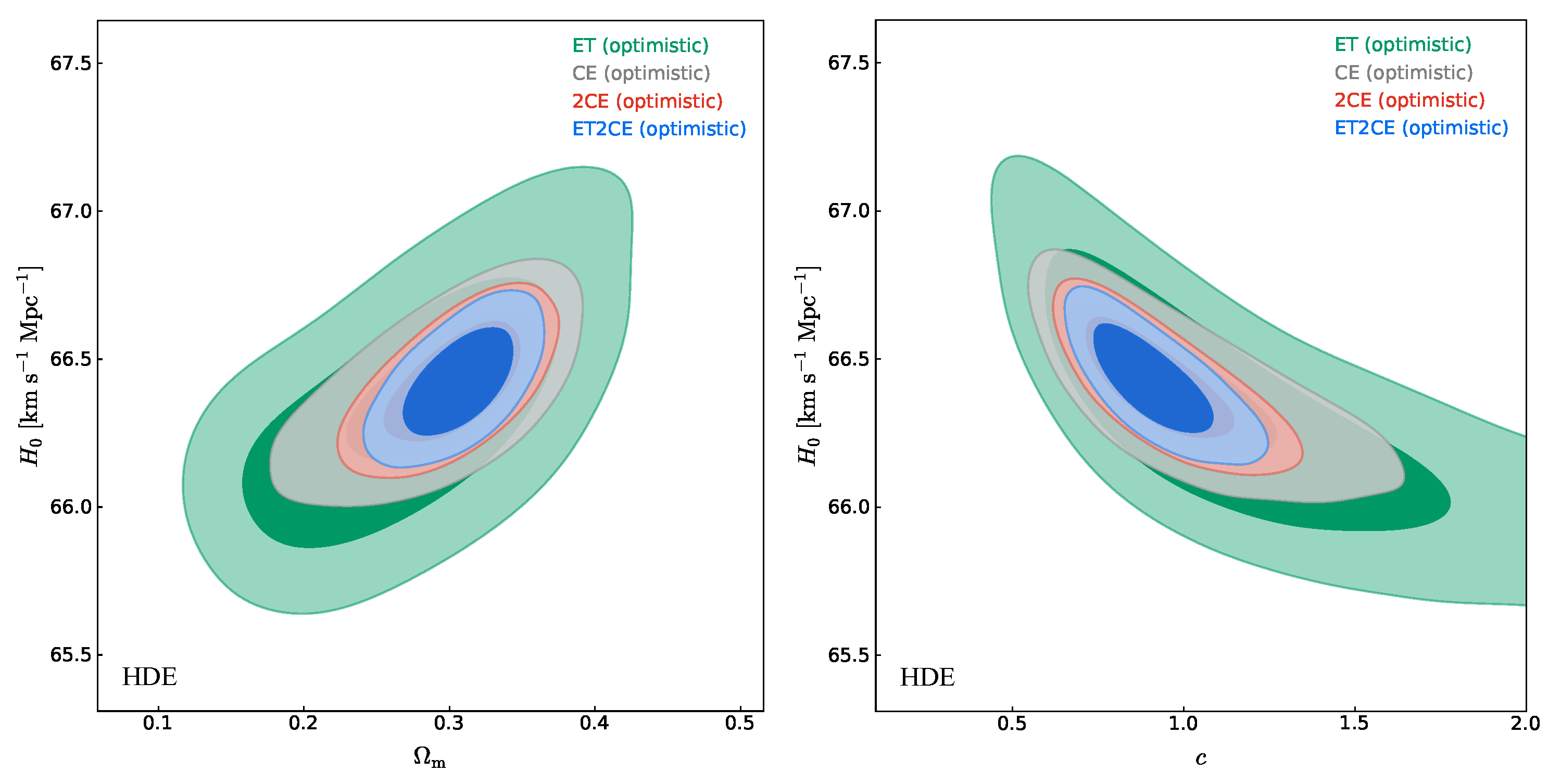
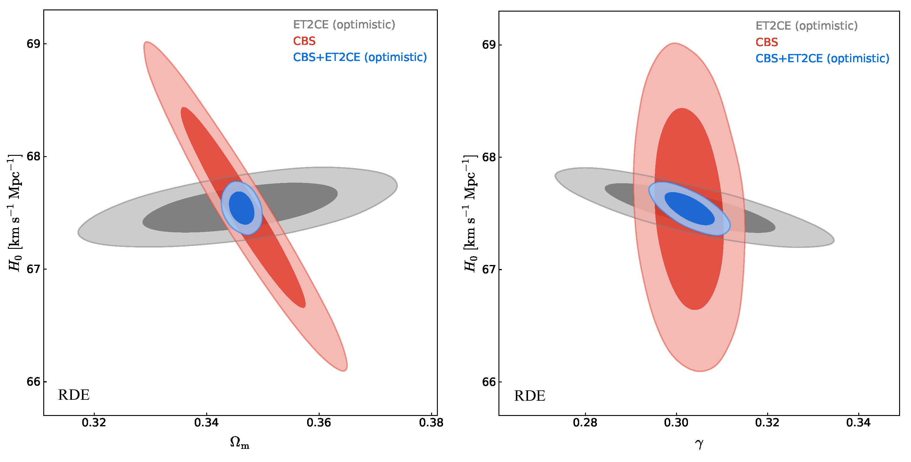
4.1. Constraint Results in Optimistic Scenario

In Figure 5, we show the constraint results for the HDE model. It is clear that ET2CE provides the tightest constraints, followed by 2CE, CE, and ET. The primary reason is that the constraint results are highly influenced by the numbers and errors of the standard siren data, while ET2CE offers the highest number of data points with the lowest errors, followed by 2CE, CE, and ET. Nonetheless, ET gives $\sigma \left(H_0\right)=0.295\mathrm{km}{\mathrm{s}}^{-1}{\mathrm{Mpc}}^{-1}$ with a constraint precision of $0.44\%$, which is much better than that of CBS. However, for other cosmological parameters, the GW data alone can only provide rather weak measurements. Fortunately, GW can effectively break the cosmological parameter degeneracies generated by CBS, as shown in Figure 6. As can be seen, the parameter degeneracy orientations of ET2CE and CBS are different. With the addition of ET2CE to CBS, the constraint precision of cosmological parameters is significantly improved. CBS + ET2CE gives $\sigma \left(c\right)=0.0023$ and $\sigma \left(H_0\right)=0.079\mathrm{km}{\mathrm{s}}^{-1}{\mathrm{Mpc}}^{-1}$, which are $43.9\%$ and $88.4\%$ better than those of CBS. In addition, the constraint precisions of ${\Omega }_{\mathrm{m}}$ and $H_0$ are $0.64\%$ and $0.12\%$, both of which are significantly better than $1\%$, the standard of precision cosmology. Meanwhile, from Figure 6, we can also find that the central value of c given by CBS is 0.887. Since $c<1$, the EoS of dark energy in the HDE model crosses the phantom divide of $w=-1$, which means that the current and future universe is dominated by phantom energy and will end up with a “big rip” singularity. Since the GW data are simulated based on the CBS constraints, the combination of CBS and GW cannot affect the central value of c, but it can reduce the error of c. For the same reason, this paper does not address the consistency between GW and CBS (including the latest DESI BAO) constraints.

In Figure 7, we show the constraint results for the RDE model. The constraint results for GW still hold, with ET2CE providing the tightest constraints, followed by 2CE, CE, and ET. For the constraint precision of the parameters ${\Omega }_{\mathrm{m}}$, ET2CE gives ${\Omega }_{\mathrm{m}}=0.0110$, which is slightly worse than that of CBS. With the addition of ET2CE to CBS, the constraints on $\gamma$ and $H_0$ could be improved by $28.0\%$ and $83.6\%$. Meanwhile, CBS + ET2CE gives $\sigma \left(\gamma \right)=0.0036$ with a precision of $1.19\%$, which is nearly at the level expected in precision cosmology. It is promising that the fundamental nature of dark energy could be explored using 3G GW standard sirens.

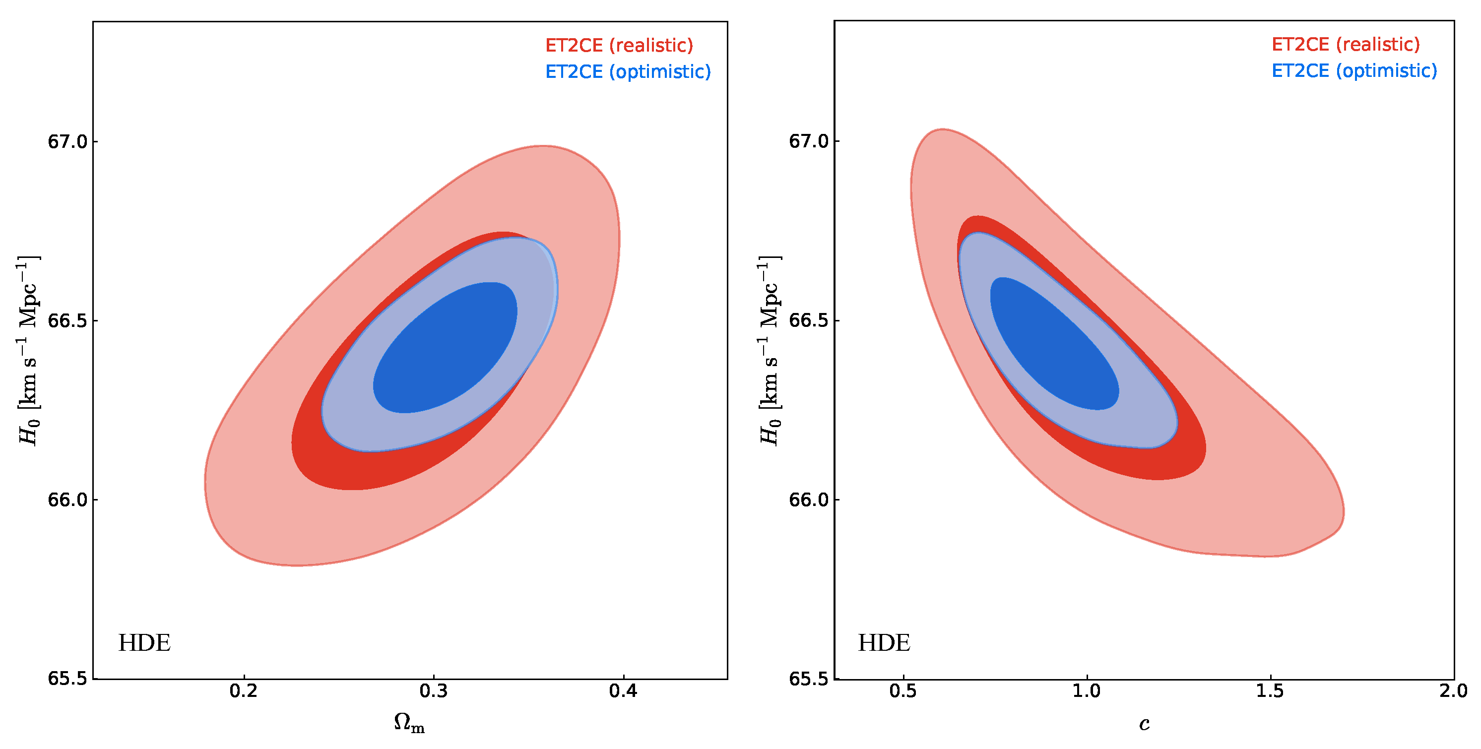
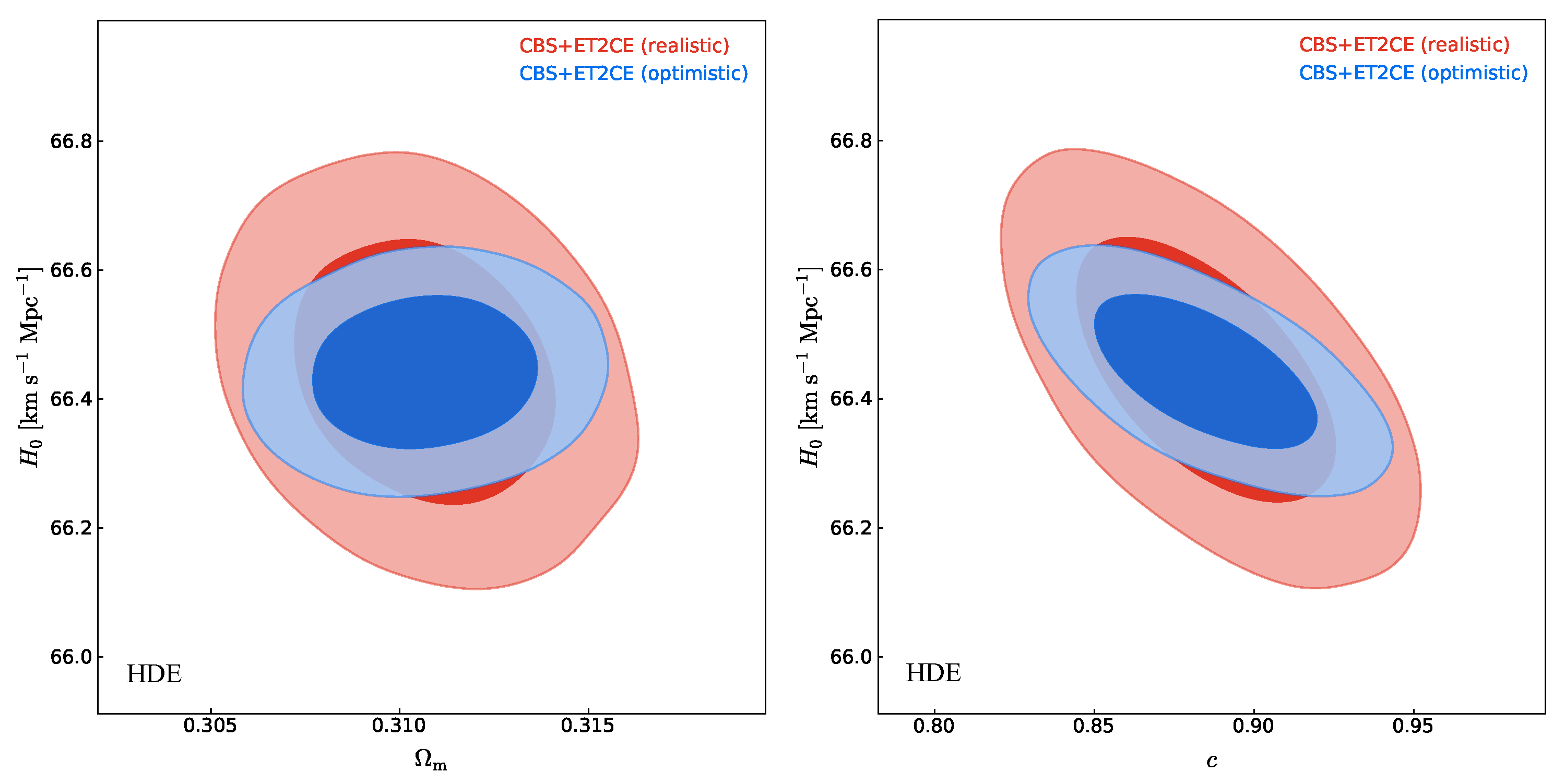
4.2. Constraint Results in Realistic Scenario

In Figure 8 and Figure 9, we present the constraint results for the HDE model. In Figure 8, we can clearly find that ET2CE (optimistic) gives tighter constraint results than those of ET2CE (realistic). ET2CE (realistic) givens $\sigma \left(c\right)=0.220$ and $\sigma \left(H_0\right)=0.24$, which are $93.0\%$ and $100.0\%$ worse than those of ET2CE (optimistic). In Figure 9, we can find that CBS + ET2CE (optimistic) also gives tighter constraints on cosmological parameters than those of CBS + ET2CE (realistic). CBS + ET2CE (realistic) givens $\sigma \left(c\right)=0.027$ and $\sigma \left(H_0\right)=0.14$, which are $17.4\%$ and $77.2\%$ worse than those of CBS + ET2CE (optimistic). In Figure 10, we show the case of the RDE model. We can also find that CBS + ET2CE (optimistic) gives tighter constraints on cosmological parameters than those of CBS + ET2CE (realistic). CBS + ET2CE (realistic) givens $\sigma \left(\gamma \right)=0.0043$ and $\sigma \left(H_0\right)=0.15$, which are $19.4\%$ and $54.6\%$ worse than those of CBS + ET2CE (optimistic).

4.3. Methodological Improvements Compared to Previous Work

Compared to previous work [70], the main differences in our methodological improvements are as follows.

In previous paper, it was commonly assumed that there will be around 1000 standard sirens with detectable EM counterparts for either ET or CE alone over a 10-year observation. However, this assumption is overly optimistic and may not be realistic. For instance, despite the optimistic estimate for a single ET detector, we expect only about 252 detectable GW-GRB events. Even with the ET2CE network, the number of detectable GW-GRB events is 363. This clearly indicates that the number of standard sirens has been considerably overestimated in previous paper.

Previous work typically assumed that the redshift distribution of standard sirens directly followed the one derived from the star formation rate, which had long tails at higher redshifts. However, in joint GW-GRB observations, the detection rates of both GW and GRB detectors for events across different redshifts must be taken into account. As a result, the redshift distribution in our analysis is shifted to lower values, primarily within the range $z\in [0,2]$, as shown in Figure 1 and Figure 2, rather than extending up to $z\in [0,5]$.

In previous paper, the influence of Earth’s rotation was overlooked. However, considering the significant impact of this effect on 3G GW detectors [74], we incorporate Earth’s rotational effects in our simulation of GW standard sirens to more accurately represent real observational conditions.

In this work, we use the updated “Pantheon+” compilation [115], which includes 1701 light curves from 1550 distinct objects, compared to the earlier “Pantheon” dataset with 1048 data points [122]. This upgrade significantly improves the constraining power of Pantheon+ relative to the original Pantheon dataset.

4.4. Constraint Results Compared to Previous Works

In Ref. [70] for ET alone in the HDE model, they gave $\sigma \left(H_0\right)=0.59\mathrm{km}{\mathrm{s}}^{-1}{\mathrm{Mpc}}^{-1}$, which is worse than our constraint result under the realistic scenario. However, for the parameter ${\Omega }_{\mathrm{m}}$, they gave $\sigma \left({\Omega }_{\mathrm{m}}\right)=0.0306$, which is tighter than our result under the optimistic scenario. This is primarily due to the fact that, compared to previous work, the redshift distributions of GW standard sirens in our analysis are lower, as mentioned above. In the early universe, the expansion history is dominated by ${\Omega }_{\mathrm{m}}$, which makes low-redshift GW events less effective at constraining ${\Omega }_{\mathrm{m}}$. On the other hand, low-redshift GW events primarily capture the direct effects of the Hubble constant $H_0$, thus providing stronger constraints on $H_0$. For the parameter c, they gave $\sigma \left(c\right)=0.218$, which is tighter than our optimistic scenario result. Similar conclusions generally hold for the RDE model. It should be noted that, when combined with CBS, our constraint results under the realistic scenario provide better or slightly better constraints than those presented in their analysis. This is primarily because, for SN data, we utilized the updated “Pantheon+” dataset, which provides stronger constraints than the “Pantheon” dataset used in their analysis.

Then, we turn our attention to the wCDM and I$\Lambda$CDM models, which also contain just one extra parameter compared to the $\Lambda$CDM model. In our previous work [74], we employed a similar methodology to obtain the constraint results for both the wCDM and I$\Lambda$CDM ($Q=\beta H{\rho }_c$) models. For ET alone in the wCDM model, we obtained $\sigma \left(w\right)=0.120$ under the optimistic scenario, which is slightly tighter than the constraint results provided by Zhang et al. [70]. In the I$\Lambda$CDM model, under the realistic scenario with CBS + ET, we obtained $\sigma \left(\beta \right)=0.00081$, which is better than the result given by Li et al. [67], who adopted a methodology similar to Zhang et al. [70].

4.5. Challenges of the HDE Model

Recently, Li et al. [31] investigated the cosmological implications of the HDE model using CMB power spectrum, DESI 2024 BAO, and SN data. They found that when evaluated with DESI BAO and SN data, the HDE model performs comparably to the $\Lambda$CDM model based on the Bayesian evidence. However, the inclusion of CMB data makes the HDE model significantly less favored than the $\Lambda$CDM model, although this is not sufficient to definitively refute the HDE model. In addition, the systematic errors in CMB observation (e.g., the measurement of temperature or polarization) may also affect this conclusion. Therefore, despite challenges posed by current observations, the HDE model has not been definitively excluded. It merits further investigation, particularly with the availability of more precise late-universe observations in the future, especially GW observations, which could offer critical insights into the nature of dark energy.

In addition, the holographic principle may also encounter observational challenges. It is noted that quantum fluctuations in spacetime would lead to apparent “holographic noise”, which is measurable by GW detectors [123]. The GEO600 detector observed unexplained “mysterious noise” in its most sensitive frequency range of 300–1400 Hz, with a spectrum roughly consistent with the predictions of holographic noise [124]. However, analyses in 2011 of measurements of GRB 041219A failed to detect holographic noise at the expected scale [125]. Despite these challenges, the holographic principle remains an intriguing area of investigation, as it offers a potential framework for understanding quantum gravity and could provide new insights in the future with more refined experiments and observations.

5. Conclusions

In this paper, we investigate the ability of 3G GW detectors to constrain HDE and RDE models using GW standard sirens. We examine the synergy between 3G GW detectors and the THESEUS-like GRB detector for multi-messenger observations. Specifically, we evaluate four detection strategies: ET, CE, the 2CE network, and the ET2CE network. Additionally, we consider both optimistic (all detected short GRBs can determine redshifts) and realistic (only 1/3 of detected short GRBs can determine redshifts) scenarios for the FoV in order to conduct the multi-messenger analysis.

We find that GW data alone can provide tight constraints on $H_0$, with precision of 0.18–0.64% in the HDE model. However, it offers loose constraints on other cosmological parameters. Fortunately, due to its ability to break parameter degeneracies generated by other EM observations, GW can play a vital role in improving the overall parameter estimation. With the addition of GW to CBS, the constraints on cosmological parameters $H_0$, c and ${\Omega }_{\mathrm{m}}$ can be improved by $63.2$–$88.4\%$, $26.8$–$43.9\%$ and $55.2$–$70.1\%$ in the HDE model. Additionally, although current observations have already excluded the RDE model, the use of GW data will further enhance the accuracy of parameter estimation for this model.

References

1. Riess, A.G.; Filippenko, A.V.; Challis, P.; Clocchiatti, A.; Diercks, A.; Garnavich, P.M.; Gilliland, R.L.; Hogan, C.J.; Jha, S.; Kirshner, R.P.; et al. Observational evidence from supernovae for an accelerating universe and a cosmological constant. Astron. J. 1998, 116, 1009–1038. [Google Scholar] [CrossRef]
2. Perlmutter, S.; Aldering, G.; Goldhaber, G.; Knop, R.A.; Nugent, P.; Castro, P.G.; Deustua, S.; Fabbro, S.; Goobar, A.; Groom, D.E.; et al. Measurements of Ω and Λ from 42 high redshift supernovae. Astrophys. J. 1999, 517, 565–586. [Google Scholar] [CrossRef]
3. Sahni, V.; Starobinsky, A.A. The Case for a positive cosmological Lambda term. Int. J. Mod. Phys. D 2000, 9, 373–444. [Google Scholar] [CrossRef]
4. Caldwell, R.R. A Phantom menace? Phys. Lett. B 2002, 545, 23–29. [Google Scholar] [CrossRef]
5. Padmanabhan, T. Cosmological constant: The Weight of the vacuum. Phys. Rept. 2003, 380, 235–320. [Google Scholar] [CrossRef]
6. Peebles, P.J.E.; Ratra, B. The Cosmological Constant and Dark Energy. Rev. Mod. Phys. 2003, 75, 559–606. [Google Scholar] [CrossRef]
7. Copeland, E.J.; Sami, M.; Tsujikawa, S. Dynamics of dark energy. Int. J. Mod. Phys. D 2006, 15, 1753–1936. [Google Scholar] [CrossRef]
8. Li, M.; Li, X.D.; Wang, S.; Wang, Y. Dark Energy. Commun. Theor. Phys. 2011, 56, 525–604. [Google Scholar] [CrossRef]
9. Bamba, K.; Capozziello, S.; Nojiri, S.; Odintsov, S.D. Dark energy cosmology: The equivalent description via different theoretical models and cosmography tests. Astrophys. Space Sci. 2012, 342, 155–228. [Google Scholar] [CrossRef]
10. Weinberg, S. The Cosmological Constant Problem. Rev. Mod. Phys. 1989, 61, 1–23. [Google Scholar] [CrossRef]
11. Carroll, S.M. The Cosmological constant. Living Rev. Rel. 2001, 4, 1. [Google Scholar] [CrossRef]
12. Li, M. A Model of holographic dark energy. Phys. Lett. B 2004, 603, 1. [Google Scholar] [CrossRef]
13. Cohen, A.G.; Kaplan, D.B.; Nelson, A.E. Effective field theory, black holes, and the cosmological constant. Phys. Rev. Lett. 1999, 82, 4971–4974. [Google Scholar] [CrossRef]
14. Zhang, X.; Wu, F.Q. Constraints on holographic dark energy from Type Ia supernova observations. Phys. Rev. D 2005, 72, 043524. [Google Scholar] [CrossRef]
15. Zhang, X.; Wu, F.Q. Constraints on Holographic Dark Energy from Latest Supernovae, Galaxy Clustering, and Cosmic Microwave Background Anisotropy Observations. Phys. Rev. D 2007, 76, 023502. [Google Scholar] [CrossRef]
16. Huang, Q.G.; Gong, Y.G. Supernova constraints on a holographic dark energy model. JCAP 2004, 08, 006. [Google Scholar] [CrossRef]
17. Wang, B.; Abdalla, E.; Su, R.K. Constraints on the dark energy from holography. Phys. Lett. B 2005, 611, 21–26. [Google Scholar] [CrossRef]
18. Nojiri, S.; Odintsov, S.D. Unifying phantom inflation with late-time acceleration: Scalar phantom-non-phantom transition model and generalized holographic dark energy. Gen. Rel. Grav. 2006, 38, 1285–1304. [Google Scholar] [CrossRef]
19. Chang, Z.; Wu, F.Q.; Zhang, X. Constraints on holographic dark energy from x-ray gas mass fraction of galaxy clusters. Phys. Lett. B 2006, 633, 14–18. [Google Scholar] [CrossRef]
20. Zhang, J.f.; Zhang, X.; Liu, H.y. Holographic dark energy in a cyclic universe. Eur. Phys. J. C 2007, 52, 693–699. [Google Scholar] [CrossRef]
21. Li, Y.H.; Wang, S.; Li, X.D.; Zhang, X. Holographic dark energy in a Universe with spatial curvature and massive neutrinos: A full Markov Chain Monte Carlo exploration. JCAP 2013, 02, 033. [Google Scholar] [CrossRef]
22. Zhang, J.F.; Zhao, M.M.; Cui, J.L.; Zhang, X. Revisiting the holographic dark energy in a non-flat universe: Alternative model and cosmological parameter constraints. Eur. Phys. J. C 2014, 74, 3178. [Google Scholar] [CrossRef]
23. Landim, R.C.G. Holographic dark energy from minimal supergravity. Int. J. Mod. Phys. D 2016, 25, 1650050. [Google Scholar] [CrossRef]
24. Wang, S.; Wang, Y.; Li, M. Holographic Dark Energy. Phys. Rept. 2017, 696, 1–57. [Google Scholar] [CrossRef]
25. Li, M.; Li, X.; Zhang, X. Comparison of dark energy models: A perspective from the latest observational data. Sci. China Phys. Mech. Astron. 2010, 53, 1631–1645. [Google Scholar] [CrossRef]
26. Xu, Y.Y.; Zhang, X. Comparison of dark energy models after Planck 2015. Eur. Phys. J. C 2016, 76, 588. [Google Scholar] [CrossRef]
27. Li, H.L.; Zhang, J.F.; Feng, L.; Zhang, X. Reexploration of interacting holographic dark energy model: Cases of interaction term excluding the Hubble parameter. Eur. Phys. J. C 2017, 77, 907. [Google Scholar] [CrossRef]
28. Feng, L.; Li, Y.H.; Yu, F.; Zhang, J.F.; Zhang, X. Exploring interacting holographic dark energy in a perturbed universe with parameterized post-Friedmann approach. Eur. Phys. J. C 2018, 78, 865. [Google Scholar] [CrossRef]
29. Li, M.; Li, X.D.; Ma, Y.Z.; Zhang, X.; Zhang, Z. Planck Constraints on Holographic Dark Energy. JCAP 2013, 09, 021. [Google Scholar] [CrossRef]
30. Wang, S.; Li, M. Theoretical aspects of holographic dark energy. Commun. Theor. Phys. 2023, 75, 117401. [Google Scholar] [CrossRef]
31. Li, T.N.; Li, Y.H.; Du, G.H.; Wu, P.J.; Feng, L.; Zhang, J.F.; Zhang, X. Revisiting holographic dark energy after DESI 2024. arXiv 2024, arXiv:2411.08639v1. [Google Scholar] [CrossRef]
32. Nojiri, S.; Odintsov, S.D. Covariant Generalized Holographic Dark Energy and Accelerating Universe. Eur. Phys. J. C 2017, 77, 528. [Google Scholar] [CrossRef]
33. Nojiri, S.; Odintsov, S.D.; Oikonomou, V.K.; Paul, T. Unifying Holographic Inflation with Holographic Dark Energy: A Covariant Approach. Phys. Rev. D 2020, 102, 023540. [Google Scholar] [CrossRef]
34. Nojiri, S.; Odintsov, S.D.; Paul, T. Different Faces of Generalized Holographic Dark Energy. Symmetry 2021, 13, 928. [Google Scholar] [CrossRef]
35. Nojiri, S.; Odintsov, S.D.; Paul, T. Barrow entropic dark energy: A member of generalized holographic dark energy family. Phys. Lett. B 2022, 825, 136844. [Google Scholar] [CrossRef]
36. Nojiri, S.; Odintsov, S.D.; Saridakis, E.N. Holographic inflation. Phys. Lett. B 2019, 797, 134829. [Google Scholar] [CrossRef]
37. Gao, C.; Wu, F.; Chen, X.; Shen, Y.G. A Holographic Dark Energy Model from Ricci Scalar Curvature. Phys. Rev. D 2009, 79, 043511. [Google Scholar] [CrossRef]
38. Zhang, X. Holographic Ricci dark energy: Current observational constraints, quintom feature, and the reconstruction of scalar-field dark energy. Phys. Rev. D 2009, 79, 103509. [Google Scholar] [CrossRef]
39. Cai, R.G.; Hu, B.; Zhang, Y. Holography, UV/IR Relation, Causal Entropy Bound and Dark Energy. Commun. Theor. Phys. 2009, 51, 954–960. [Google Scholar] [CrossRef]
40. Fu, T.F.; Zhang, J.F.; Chen, J.Q.; Zhang, X. Holographic Ricci dark energy: Interacting model and cosmological constraints. Eur. Phys. J. C 2012, 72, 1932. [Google Scholar] [CrossRef]
41. Cui, J.L.; Zhang, J.F. Comparing holographic dark energy models with statefinder. Eur. Phys. J. C 2014, 74, 2849. [Google Scholar] [CrossRef]
42. Zhang, J.F.; Cui, J.L.; Zhang, X. Diagnosing holographic dark energy models with statefinder hierarchy. Eur. Phys. J. C 2014, 74, 3100. [Google Scholar] [CrossRef]
43. Yu, F.; Cui, J.L.; Zhang, J.F.; Zhang, X. Statefinder hierarchy exploration of the extended Ricci dark energy. Eur. Phys. J. C 2015, 75, 274. [Google Scholar] [CrossRef]
44. Riess, A.G.; Yuan, W.; Macri, L.M.; Scolnic, D.; Brout, D.; Casertano, S.; Jones, D.O.; Murakami, Y.; Anand, G.S.; Breuval, L.; et al. A Comprehensive Measurement of the Local Value of the Hubble Constant with 1 km s-1 Mpc-1 Uncertainty from the Hubble Space Telescope and the SH0ES Team. Astrophys. J. Lett. 2022, 934, L7. [Google Scholar] [CrossRef]
45. Cai, R.G. Editorial. Sci. China Phys. Mech. Astron. 2020, 63, 290401. [Google Scholar] [CrossRef]
46. Guo, R.Y.; Zhang, J.F.; Zhang, X. Inflation model selection revisited after a 1.91% measurement of the Hubble constant. Sci. China Phys. Mech. Astron. 2020, 63, 290406. [Google Scholar] [CrossRef]
47. Yang, W.; Pan, S.; Di Valentino, E.; Nunes, R.C.; Vagnozzi, S.; Mota, D.F. Tale of stable interacting dark energy, observational signatures, and the H0 tension. JCAP 2018, 09, 019. [Google Scholar] [CrossRef]
48. Vagnozzi, S. New physics in light of the H0 tension: An alternative view. Phys. Rev. D 2020, 102, 023518. [Google Scholar] [CrossRef]
49. Di Valentino, E.; Melchiorri, A.; Mena, O.; Vagnozzi, S. Nonminimal dark sector physics and cosmological tensions. Phys. Rev. D 2020, 101, 063502. [Google Scholar] [CrossRef]
50. Di Valentino, E.; Melchiorri, A.; Mena, O.; Vagnozzi, S. Interacting dark energy in the early 2020s: A promising solution to the H0 and cosmic shear tensions. Phys. Dark Univ. 2020, 30, 100666. [Google Scholar] [CrossRef]
51. Liu, M.; Huang, Z.; Luo, X.; Miao, H.; Singh, N.K.; Huang, L. Can Non-standard Recombination Resolve the Hubble Tension? Sci. China Phys. Mech. Astron. 2020, 63, 290405. [Google Scholar] [CrossRef]
52. Zhang, X.; Huang, Q.G. Measuring H0 from low-z datasets. Sci. China Phys. Mech. Astron. 2020, 63, 290402. [Google Scholar] [CrossRef]
53. Ding, Q.; Nakama, T.; Wang, Y. A gigaparsec-scale local void and the Hubble tension. Sci. China Phys. Mech. Astron. 2020, 63, 290403. [Google Scholar] [CrossRef]
54. Lin, M.X.; Hu, W.; Raveri, M. Testing H0 in Acoustic Dark Energy with Planck and ACT Polarization. Phys. Rev. D 2020, 102, 123523. [Google Scholar] [CrossRef]
55. Hryczuk, A.; Jodłowski, K. Self-interacting dark matter from late decays and the H0 tension. Phys. Rev. D 2020, 102, 043024. [Google Scholar] [CrossRef]
56. Cai, R.G.; Guo, Z.K.; Li, L.; Wang, S.J.; Yu, W.W. Chameleon dark energy can resolve the Hubble tension. Phys. Rev. D 2021, 103, 121302. [Google Scholar] [CrossRef]
57. Vagnozzi, S.; Pacucci, F.; Loeb, A. Implications for the Hubble tension from the ages of the oldest astrophysical objects. JHEAp 2022, 36, 27–35. [Google Scholar] [CrossRef]
58. Vagnozzi, S. Consistency tests of ΛCDM from the early integrated Sachs-Wolfe effect: Implications for early-time new physics and the Hubble tension. Phys. Rev. D 2021, 104, 063524. [Google Scholar] [CrossRef]
59. Riess, A.G. The Expansion of the Universe is Faster than Expected. Nat. Rev. Phys. 2019, 2, 10–12. [Google Scholar] [CrossRef]
60. Verde, L.; Treu, T.; Riess, A.G. Tensions between the Early and the Late Universe. Nat. Astron. 2019, 3, 891. [Google Scholar] [CrossRef]
61. Li, T.N.; Wu, P.J.; Du, G.H.; Jin, S.J.; Li, H.L.; Zhang, J.F.; Zhang, X. Constraints on Interacting Dark Energy Models from the DESI Baryon Acoustic Oscillation and DES Supernovae Data. Astrophys. J. 2024, 976, 1. [Google Scholar] [CrossRef]
62. Schutz, B.F. Determining the Hubble Constant from Gravitational Wave Observations. Nature 1986, 323, 310–311. [Google Scholar] [CrossRef]
63. Holz, D.E.; Hughes, S.A. Using gravitational-wave standard sirens. Astrophys. J. 2005, 629, 15–22. [Google Scholar] [CrossRef]
64. Zhao, W.; Van Den Broeck, C.; Baskaran, D.; Li, T.G.F. Determination of Dark Energy by the Einstein Telescope: Comparing with CMB, BAO and SNIa Observations. Phys. Rev. D 2011, 83, 023005. [Google Scholar] [CrossRef]
65. Zhang, X.N.; Wang, L.F.; Zhang, J.F.; Zhang, X. Improving cosmological parameter estimation with the future gravitational-wave standard siren observation from the Einstein Telescope. Phys. Rev. D 2019, 99, 063510. [Google Scholar] [CrossRef]
66. Jin, S.J.; He, D.Z.; Xu, Y.; Zhang, J.F.; Zhang, X. Forecast for cosmological parameter estimation with gravitational-wave standard siren observation from the Cosmic Explorer. JCAP 2020, 03, 051. [Google Scholar] [CrossRef]
67. Li, H.L.; He, D.Z.; Zhang, J.F.; Zhang, X. Quantifying the impacts of future gravitational-wave data on constraining interacting dark energy. JCAP 2020, 06, 038. [Google Scholar] [CrossRef]
68. Cai, R.G.; Liu, T.B.; Liu, X.W.; Wang, S.J.; Yang, T. Probing cosmic anisotropy with gravitational waves as standard sirens. Phys. Rev. D 2018, 97, 103005. [Google Scholar] [CrossRef]
69. Cai, R.G.; Yang, T. Estimating cosmological parameters by the simulated data of gravitational waves from the Einstein Telescope. Phys. Rev. D 2017, 95, 044024. [Google Scholar] [CrossRef]
70. Zhang, J.F.; Dong, H.Y.; Qi, J.Z.; Zhang, X. Prospect for constraining holographic dark energy with gravitational wave standard sirens from the Einstein Telescope. Eur. Phys. J. C 2020, 80, 217. [Google Scholar] [CrossRef]
71. Jin, S.J.; Zhang, Y.Z.; Song, J.Y.; Zhang, J.F.; Zhang, X. Taiji-TianQin-LISA network: Precisely measuring the Hubble constant using both bright and dark sirens. Sci. China Phys. Mech. Astron. 2024, 67, 220412. [Google Scholar] [CrossRef]
72. Abbott, B.P.; Abbott, R.; Abbott, T.D.; Abraham, S.; Acernese, F.; Ackley, K.; Adams, C.; Adya, V.B.; Affeldt, C.; Agathos, M.; et al. Prospects for observing and localizing gravitational-wave transients with Advanced LIGO, Advanced Virgo and KAGRA. Living Rev. Rel. 2018, 21, 3. [Google Scholar] [CrossRef]
73. Song, J.Y.; Wang, L.F.; Li, Y.; Zhao, Z.W.; Zhang, J.F.; Zhao, W.; Zhang, X. Synergy between CSST galaxy survey and gravitational-wave observation: Inferring the Hubble constant from dark standard sirens. Sci. China Phys. Mech. Astron. 2024, 67, 230411. [Google Scholar] [CrossRef]
74. Han, T.; Jin, S.J.; Zhang, J.F.; Zhang, X. A comprehensive forecast for cosmological parameter estimation using joint observations of gravitational waves and short γ-ray bursts. Eur. Phys. J. C 2024, 84, 663. [Google Scholar] [CrossRef]
75. Abbott, B.P.; Abbott, R.; Adhikari, R.X.; Ananyeva, A.; Anderson, S.B.; Appert, S.; Arai, K.; Araya, M.C.; Barayoga, J.C.; Barish, B.C.; et al. A gravitational-wave standard siren measurement of the Hubble constant. Nature 2017, 551, 85–88. [Google Scholar] [CrossRef]
76. ET. Available online: https://www.et-gw.eu (accessed on 5 March 2025).
77. Punturo, M.; Abernathy, M.; Acernese, F.; Allen, B.; Andersson, N.; Arun, K.; Barone, F.; Barr, B.; Barsuglia, M.; Beker, M.; et al. The Einstein Telescope: A third-generation gravitational wave observatory. Class. Quant. Grav. 2010, 27, 194002. [Google Scholar] [CrossRef]
78. CE. Available online: https://cosmicexplorer.org/ (accessed on 5 March 2025).
79. Abbott, B.P.; Abbott, R.; Abbott, T.D.; Abernathy, M.R.; Ackley, K.; Adams, C.; Addesso, P.; Adhikari, R.X.; Adya, V.B.; Affeldt, C.; et al. Exploring the Sensitivity of Next Generation Gravitational Wave Detectors. Class. Quant. Grav. 2017, 34, 044001. [Google Scholar] [CrossRef]
80. Evans, M.; Adhikari, R.X.; Afle, C.; Ballmer, S.W.; Biscoveanu, S.; Borhanian, S.; Brown, D.A.; Chen, Y.; Eisenstein, R.; Gruson, A.; et al. A Horizon Study for Cosmic Explorer: Science, Observatories, and Community. arXiv 2021, arXiv:2109.09882. [Google Scholar] [CrossRef]
81. Amati, L.; O’Brien, P.T.; Götz, D.; Bozzo, E.; Santangelo, A.; Tanvir, N.; Frontera, F.; Mereghetti, S.; Osborne, J.P.; Blain, A.; et al. The THESEUS space mission: Science goals, requirements and mission concept. Exper. Astron. 2021, 52, 183–218. [Google Scholar] [CrossRef]
82. Amati, L.; O’Brien, P.; Götz, D.; Bozzo, E.; Tenzer, C.; Frontera, F.; Ghirlanda, G.; Labanti, C.; Osborne, J.P.; Stratta, G.; et al. The THESEUS space mission concept: Science case, design and expected performances. Adv. Space Res. 2018, 62, 191–244. [Google Scholar] [CrossRef]
83. Stratta, G.; Ciolfi, R.; Amati, L.; Bozzo, E.; Ghirlanda, G.; Maiorano, E.; Nicastro, L.; Rossi, A.; Vinciguerra, S.; Frontera, F.; et al. THESEUS: A key space mission concept for Multi-Messenger Astrophysics. Adv. Space Res. 2018, 62, 662–682. [Google Scholar] [CrossRef]
84. Stratta, G.; Amati, L.; Ciolfi, R.; Vinciguerra, S. THESEUS in the era of Multi-Messenger Astronomy. Mem. Soc. Ast. It. 2018, 89, 205–212. [Google Scholar] [CrossRef]
85. ’t Hooft, G. Dimensional reduction in quantum gravity. Conf. Proc. C 1993, 930308, 284–296. [Google Scholar] [CrossRef]
86. Susskind, L. The World as a hologram. J. Math. Phys. 1995, 36, 6377–6396. [Google Scholar] [CrossRef]
87. Vitale, S.; Farr, W.M.; Ng, K.; Rodriguez, C.L. Measuring the star formation rate with gravitational waves from binary black holes. Astrophys. J. Lett. 2019, 886, L1. [Google Scholar] [CrossRef]
88. Belgacem, E.; Dirian, Y.; Foffa, S.; Howell, E.J.; Maggiore, M.; Regimbau, T. Cosmology and dark energy from joint gravitational wave-GRB observations. JCAP 2019, 08, 015. [Google Scholar] [CrossRef]
89. Yang, T. Gravitational-Wave Detector Networks: Standard Sirens on Cosmology and Modified Gravity Theory. JCAP 2021, 05, 044. [Google Scholar] [CrossRef]
90. Madau, P.; Dickinson, M. Cosmic Star Formation History. Ann. Rev. Astron. Astrophys. 2014, 52, 415–486. [Google Scholar] [CrossRef]
91. Virgili, F.J.; Zhang, B.; O’Brien, P.; Troja, E. Are all short-hard gamma-ray bursts produced from mergers of compact stellar objects? Astrophys. J. 2011, 727, 109. [Google Scholar] [CrossRef]
92. D’Avanzo, P.; Salvaterra, R.; Bernardini, M.G.; Nava, L.; Campana, S.; Covino, S.; D’Elia, V.; Ghirlanda, G.; Ghisellini, G.; Melandri, A.; et al. A complete sample of bright Swift short Gamma-Ray Bursts. Mon. Not. Roy. Astron. Soc. 2014, 442, 2342–2356. [Google Scholar] [CrossRef]
93. Abbott, B.P.; Abbott, R.; Abbott, T.; Abraham, S.; Acernese, F.; Ackley, K.; Adams, C.; Adhikari, R.; Adya, V.; LIGO Scientific Collaboration and Virgo Collaboration; et al. GWTC-1: A Gravitational-Wave Transient Catalog of Compact Binary Mergers Observed by LIGO and Virgo during the First and Second Observing Runs. Phys. Rev. X 2019, 9, 031040. [Google Scholar] [CrossRef]
94. Abbott, R.; Abbott, T.; Acernese, F.; Ackley, K.; Adams, C.; Adhikari, N.; Adhikari, R.; Adya, V.; Affeldt, C.; LIGO Scientific Collaboration, Virgo Collaboration, and KAGRA Collaboration; et al. Population of Merging Compact Binaries Inferred Using Gravitational Waves through GWTC-3. Phys. Rev. X 2023, 13, 011048. [Google Scholar] [CrossRef]
95. Wen, L.; Chen, Y. Geometrical Expression for the Angular Resolution of a Network of Gravitational-Wave Detectors. Phys. Rev. D 2010, 81, 082001. [Google Scholar] [CrossRef]
96. Cutler, C.; Apostolatos, T.A.; Bildsten, L.; Finn, L.S.; Flanagan, E.E.; Kennefick, D.; Markovic, D.M.; Ori, A.; Poisson, E. The Last three minutes: Issues in gravitational wave measurements of coalescing compact binaries. Phys. Rev. Lett. 1993, 70, 2984–2987. [Google Scholar] [CrossRef]
97. Sathyaprakash, B.S.; Schutz, B.F. Physics, Astrophysics and Cosmology with Gravitational Waves. Living Rev. Rel. 2009, 12, 2. [Google Scholar] [CrossRef]
98. Zhao, W.; Wen, L. Localization accuracy of compact binary coalescences detected by the third-generation gravitational-wave detectors and implication for cosmology. Phys. Rev. D 2018, 97, 064031. [Google Scholar] [CrossRef]
99. Blanchet, L.; Iyer, B.R. Hadamard regularization of the third post-Newtonian gravitational wave generation of two point masses. Phys. Rev. D 2005, 71, 024004. [Google Scholar] [CrossRef]
100. Maggiore, M. Gravitational Waves. Vol. 1: Theory and Experiments; Oxford Master Series in Physics; Oxford University Press: Oxford, UK, 2007. [Google Scholar]
101. Howell, E.J.; Ackley, K.; Rowlinson, A.; Coward, D. Joint gravitational wave—Gamma-ray burst detection rates in the aftermath of GW170817. Mon. Not. R. Astron. Soc. 2018. [Google Scholar] [CrossRef]
102. Wanderman, D.; Piran, T. The rate, luminosity function and time delay of non-Collapsar short GRBs. Mon. Not. Roy. Astron. Soc. 2015, 448, 3026–3037. [Google Scholar] [CrossRef]
103. Meszaros, P.; Meszaros, A. The Brightness distribution of bursting sources in relativistic cosmologies. Astrophys. J. 1995, 449, 9–16. [Google Scholar] [CrossRef]
104. Meszaros, A.; Ripa, J.; Ryde, F. Cosmological effects on the observed flux and fluence distributions of gamma-ray bursts: Are the most distant bursts in general the faintest ones? Astron. Astrophys. 2011, 529, A55. [Google Scholar] [CrossRef]
105. Band, D.L. Comparison of the gamma-ray burst sensitivity of different detectors. Astrophys. J. 2003, 588, 945–951. [Google Scholar] [CrossRef]
106. Hirata, C.M.; Holz, D.E.; Cutler, C. Reducing the weak lensing noise for the gravitational wave Hubble diagram using the non-Gaussianity of the magnification distribution. Phys. Rev. D 2010, 81, 124046. [Google Scholar] [CrossRef]
107. Tamanini, N.; Caprini, C.; Barausse, E.; Sesana, A.; Klein, A.; Petiteau, A. Science with the space-based interferometer eLISA. III: Probing the expansion of the Universe using gravitational wave standard sirens. JCAP 2016, 04, 002. [Google Scholar] [CrossRef]
108. Speri, L.; Tamanini, N.; Caldwell, R.R.; Gair, J.R.; Wang, B. Testing the Quasar Hubble Diagram with LISA Standard Sirens. Phys. Rev. D 2021, 103, 083526. [Google Scholar] [CrossRef]
109. Kocsis, B.; Frei, Z.; Haiman, Z.; Menou, K. Finding the electromagnetic counterparts of cosmological standard sirens. Astrophys. J. 2006, 637, 27–37. [Google Scholar] [CrossRef]
110. He, J.H. Accurate method to determine the systematics due to the peculiar velocities of galaxies in measuring the Hubble constant from gravitational-wave standard sirens. Phys. Rev. D 2019, 100, 023527. [Google Scholar] [CrossRef]
111. Chen, L.; Huang, Q.G.; Wang, K. Distance Priors from Planck Final Release. JCAP 2019, 02, 028. [Google Scholar] [CrossRef]
112. Beutler, F.; Blake, C.; Colless, M.; Jones, D.H.; Staveley-Smith, L.; Campbell, L.; Parker, Q.; Saunders, W.; Watson, F. The 6dF Galaxy Survey: Baryon Acoustic Oscillations and the Local Hubble Constant. Mon. Not. Roy. Astron. Soc. 2011, 416, 3017–3032. [Google Scholar] [CrossRef]
113. Ross, A.J.; Samushia, L.; Howlett, C.; Percival, W.J.; Burden, A.; Manera, M. The clustering of the SDSS DR7 main Galaxy sample – I. A 4 per cent distance measure at z=0.15. Mon. Not. Roy. Astron. Soc. 2015, 449, 835–847. [Google Scholar] [CrossRef]
114. Alam, S.; Ata, M.; Bailey, S.; Beutler, F.; Bizyaev, D.; Blazek, J.A.; Bolton, A.S.; Brownstein, J.R.; Burden, A.; Chuang, C.; et al. The clustering of galaxies in the completed SDSS-III Baryon Oscillation Spectroscopic Survey: Cosmological analysis of the DR12 galaxy sample. Mon. Not. Roy. Astron. Soc. 2017, 470, 2617–2652. [Google Scholar] [CrossRef]
115. Brout, D.; Scolnic, D.; Popovic, B.; Riess, A.G.; Carr, A.; Zuntz, J.; Kessler, R.; Davis, T.M.; Hinton, S.; Jones, D.; et al. The Pantheon+ Analysis: Cosmological Constraints. Astrophys. J. 2022, 938, 110. [Google Scholar] [CrossRef]
116. Available online: https://www.et-gw.eu/index.php/etsensitivities/ (accessed on 5 March 2025).
117. Available online: https://cosmicexplorer.org/sensitivity.html (accessed on 5 March 2025).
118. Zhu, J.P.; Wu, S.; Yang, Y.; Liu, C.; Zhang, B.; Song, H.; Gao, H.; Cao, Z.; Yu, Y.; Kang, Y.; et al. Kilonovae and Optical Afterglows from Binary Neutron Star Mergers. II. Optimal Search Strategy for Serendipitous Observations and Target-of-opportunity Observations of Gravitational Wave Triggers. Astrophys. J. 2023, 942, 88. [Google Scholar] [CrossRef]
119. Adame, A.G.; Aguilar, J.; Ahlen, S.; Alam, S.; Alexander, D.M.; Alvarez, M.; Alves, O.; Anand, A.; Andrade, U.; Armengaud, E.; et al. DESI 2024 III: Baryon Acoustic Oscillations from Galaxies and Quasars. arXiv 2024, arXiv:2404.03000. [Google Scholar] [CrossRef]
120. Adame, A.G.; Aguilar, J.; Ahlen, S.; Alam, S.; Alexander, D.M.; Alvarez, M.; Alves, O.; Anand, A.; Andrade, U.; Armengaud, E.; et al. DESI 2024 IV: Baryon Acoustic Oscillations from the Lyman Alpha Forest. arXiv 2024, arXiv:2404.03001. [Google Scholar] [CrossRef]
121. Ahumada, R.; Prieto, C.A.; Almeida, A.; Anders, F.; Anderson, S.F.; Andrews, B.H.; Anguiano, B.; Arcodia, R.; Armengaud, E.; Aubert, M.; et al. The 16th Data Release of the Sloan Digital Sky Surveys: First Release from the APOGEE-2 Southern Survey and Full Release of eBOSS Spectra. Astrophys. J. Suppl. 2020, 249, 3. [Google Scholar] [CrossRef]
122. Scolnic, D.M.; Jones, D.O.; Rest, A.; Pan, Y.C.; Chornock, R.; Foley, R.J.; Huber, M.E.; Kessler, R.; Narayan, G.; Riess, A.G.; et al. The Complete Light-curve Sample of Spectroscopically Confirmed SNe Ia from Pan-STARRS1 and Cosmological Constraints from the Combined Pantheon Sample. Astrophys. J. 2018, 859, 101. [Google Scholar] [CrossRef]
123. Hogan, C.J. Measurement of Quantum Fluctuations in Geometry. Phys. Rev. D 2008, 77, 104031. [Google Scholar] [CrossRef]
124. Hogan, C.J. Indeterminacy of Holographic Quantum Geometry. Phys. Rev. D 2008, 78, 087501. [Google Scholar] [CrossRef]
125. Available online: https://www.esa.int/Science_Exploration/Space_Science/Integral_challenges_physics_beyond_Einstein (accessed on 5 March 2025).
Figure 1. Redshift distributions of BNS detected by THESEUS in synergy with ET, CE, 2CE, and ET2CE for a 10-year observation in the optimistic scenario.
Universe 11 00085 g001
Figure 2. Same as Figure 1, but assuming the realistic scenario.
Universe 11 00085 g002
Figure 3. Distributions of luminosity distance uncertainty Δ d L / d L of GW standard sirens for ET, CE, 2CE, and ET2CE in the optimistic scenario under the HDE model.
Universe 11 00085 g003
Figure 4. Same as Figure 3, but assuming the realistic scenario.
Universe 11 00085 g004
Figure 5. Two-dimensional marginalized contours ( 68.3 % and 95.4 % confidence level) in the Ω m H 0 and c H 0 planes for the HDE model in the optimistic scenario using ET, CE, 2CE and ET2CE, respectively.
Universe 11 00085 g005
Figure 6. Two-dimensional marginalized contours ( 68.3 % and 95.4 % confidence level) in the Ω m H 0 and c H 0 planes for the HDE model in the optimistic scenario using ET2CE, CBS and CBS + ET2CE data, respectively.
Universe 11 00085 g006
Figure 7. Two-dimensional marginalized contours ( 68.3 % and 95.4 % confidence level) in the Ω m H 0 and γ H 0 planes for the RDE model in the optimistic scenario using ET2CE, CBS and CBS + ET2CE data, respectively.
Universe 11 00085 g007
Figure 8. Two-dimensional marginalized contours ( 68.3 % and 95.4 % confidence level) in the Ω m H 0 and c H 0 planes for the HDE model in the realistic and optimistic scenarios of the ET2CE data.
Universe 11 00085 g008
Figure 9. Two-dimensional marginalized contours ( 68.3 % and 95.4 % confidence level) in the Ω m H 0 and c H 0 planes for the HDE model in the realistic and optimistic scenarios of the CBS + ET2CE data.
Universe 11 00085 g009
Figure 10. Two-dimensional marginalized contours ( 68.3 % and 95.4 % confidence level) in the Ω m H 0 and γ H 0 planes for the RDE model in the realistic and optimistic scenarios of the CBS + ET2CE data.
Universe 11 00085 g010