On the Observation of Distant Objects in General Relativity and Its Implications in Cosmology

Abstract

We carry out a careful analysis of the notion of observation of distant events in a curved Universe. This leads us to hypothesise that all measurements of our physical environment are performed with respect to a representation referential that obeys the rules of Euclidean geometry. In curved spacetime geometries, this creates a distortion of metric quantities which affects the wavelength of photons incoming from distant sources. We show that, at the scale of our galaxy, this effect is too small to be experimentally detected. At a cosmological scale, however, and in the context of the Einstein Universe, we show that it becomes measurable and offers a simple alternative explanation for most modern cosmological observations. In particular, we predict a redshift which increases as a function of the source’s distance, in a way that is consistent with Supernovae data, and the existence of a Cosmic Microwave Background whose characteristics align with the ones measured by the Planck mission. Furthermore, it accounts for the presence of well-formed galactic structures in the high-redshift Universe, as recently detected by the James Webb Space Telescope.

1. Introduction

In 1917, Albert Einstein applied his recently developed theory of general relativity to the cosmological problem, which led him to propose a finite static solution as a model of our universe. Assuming a uniform and homogeneous distribution of matter, and after introducing an additional term to his field equations, he derived a static universe of constant spherical curvature. Soon after, this model of the universe faced two major challenges. Firstly, in 1930, Eddington raised concerns about the stability of the Einstein world and demonstrated that it is in fact unstable against a small variation of the total matter density, causing it to exponentially expand or contract [1]. However, this kind of non-local perturbation is non-physical in nature, and it is still not clear today if the Einstein world is indeed unstable against perturbations having physical relevance. We defer to the very interesting chapter [2] for a detailed discussion of the matter. The description by Hubble of a linear relation between the redshift of galaxies and their distances [3] achieved to convince Einstein, at the beginning reluctant, to change his mind and accept the growing consensus on models based on the expansion of space [4,5,6]. Such models suited quite well to the small amount of observational data yet available, although the existence of an initial spacetime singularity raised important physical and philosophical questions that remain unanswered today. The discovery of a cosmic microwave background (CMB) made by Penzias and Wilson in 1964 [7] became a strong support for this theory since its characteristics are compatible with the radiation of a dense primordial plasma. In 1998, an acceleration of the expansion of the universe was detected and surprised cosmologists [8]. This led to the introduction of a dark energy that acts as a repulsive gravitational force, whose origin remains very speculative. Efforts have been made to combine all these considerations to form the standard model of cosmology $\mathrm{\Lambda }$CDM.

Alternative theories have been developed to explain the redshift of cosmological objects in a static Universe, such as tired light theory [9], but errors have been pointed out and the theory has never been commonly accepted [10]. In the current interpretation of general relativity, if we neglect hypothetical physical processes that take energy from photons, the only possible explanation for this redshift is a mechanism that acts on the metric of spacetime. As for now, there is growing evidence that this standard cosmological model has fundamental flaws. Thanks to a new generation of measurement devices, some tensions in the standard model have become increasingly apparent [11,12], and are described by many as a crisis in Cosmology. Additionally, the James Webb Space Telescope has recently discovered well-formed galactic structures in the high-redshift Universe which are difficult to explain within the current concordance model. This calls for the exploration of new ideas to make sense of Cosmological observations.

We propose to start at a fundamental level and to carry out a careful analysis of the notion of perception of distant events in curved spacetimes. As we will see, this motivates the introduction of an observer-centered referential in which the rules of Euclidean geometry apply and to postulate that all observations of our physical environment are performed with respect to this representation referential. In curved spacetime geometries, this creates a distortion of metric quantities that affects the wavelength of incoming photons. We show that, at the scale of our galaxy, this effect is too small to be experimentally detected. At a cosmological scale, however, and in the context of a static universe of closed spatial geometry, we predict that the redshift increases as a function of the distance, in a way that is consistent with Supernovae data. Finally, we show that this accounts for the existence of a Cosmic Microwave Background whose characteristics align with the one measured by the Planck mission.

2. The Perception of Distant Objects in a Curved Universe

2.1. Representation Referential

In his book Wholeness and the implicate order [13], David Bohm points out a fundamental duality of the physical reality: a world, hardly accessible to our senses, home to unfamiliar processes that he calls the implicate order, reveals itself in an unfolded, explicate order, in which measurements can be performed, and which corresponds to our everyday experience of the physical environment. Originally thought to account for the puzzling properties of quantum mechanics, these views also find an echo in general relativity. In the latter, the fundamental object is a curved 4-dimensional pseudo-Riemannian manifold in which space and time are entangled in a profound interlace. Yet in our way of representing this environment, space and time are fundamentally distinct objects, for otherwise no measurement would be possible. We will refer to this fact as the separation principle.

In this explicate world of observation, the environment is also perceived as being flat, as we are living in a locally flat portion of the universe and our brains are equipped to make linear representations of our surroundings. To this extent, Albert Einstein writes in one of his famous 1905 papers [14]:

“If a material point is at rest relatively to a system of co-ordinates, its position can be defined relatively thereto by the employment of rigid standards of measurement and the methods of Euclidean geometry, and can be expressed in Cartesian co-ordinates.”

A few years later, the development of general relativity challenged this view and introduced more sophisticated geometrical tools to describe the physical world.

Let us now take the point of view of an observer $\mathcal{O}$ living in a universe whose geometry is described by Einstein’s field equations. In order to measure quantities such as lengths and durations associated with local events, $\mathcal{O}$ can directly compare them with different measuring devices, such as a ruler or a chronometer. In Minkowskian spacetime and for objects in uniform linear motion with respect to the observer, direct comparison is not possible and a procedure was proposed by Einstein to determine the length of such an object, supposing the universality of the speed of light c. This procedure turns out to give a value in the direction of motion that is different from the length one would measure directly by comparing the object with a ruler. This is the core of special relativity. A similar procedure can be used to determine the distance between $\mathcal{O}$ and an object at rest: $\mathcal{O}$ sends a light signal in the direction of the object at time $t_0$, and waits for it to be reflected back at time $t_1$. The distance d from the object x is then defined as:

$$d={\displaystyle \frac{c(t_1-t_0)}{2}}.$$

(1)

This definition of distance extends to more general spacetime geometries and is called proper distance in the context of a static universe. We argue that this radar-defined proper distance is the only one that can be, in principle, determined experimentally without any further knowledge of the observed object, and in flat space, it clearly aligns with the Euclidean distance. Now that he is able to determine the distance of an object, our observer may ask the following question: Is there a procedure to assign lengths and durations to events situated at large distances, and how to do so? In a flat spacetime, and if the object is at rest, the answer is simple: it can be done by using the tools of Euclidean geometry. Now, in curved spacetimes, this question becomes more challenging, especially without a priori knowledge of the spacetime geometry. In order to make a consistent representation of its physical environment, we argue that the observer has to admit a representation referential $R_{obs}$, which can be constructed in the following way.

We suppose a static spacetime and an inertial system of coordinates centered at $\mathcal{O}$ such that the metric is Minkowskian at $\mathcal{O}$. As the metric does not depend on time, we can restrict our attention to its spatial component, which describes a unique 3-dimensional manifold that we denote U. We call the representation referential, denoted by $R_{obs}$, the tangent space of U at $\mathcal{O}$. Let now $x\in U$ be a point at proper distance $d_U$ from $\mathcal{O}$. We define $T\left(x\right):U\to R_{obs}$ the representation map, which transforms a point $x\in U$ to the point $T\left(x\right)$ in $R_{obs}$1 situated at distance $d_R=d_U:=d$ from $\mathcal{O}$ and such that the vector $\overrightarrow{\mathcal{O}T}\left(x\right)$ has the same initial direction as that of the minimal geodesic connecting $\mathcal{O}$ to x in U. Whenever T is invertible, any object $X\subset U$ has a unique representation $T\left(X\right)$ in $R_{obs}$ and $T^{-1}$ is given by the exponential map at $\mathcal{O}$. We emphasise that the representation referential $R_{obs}$ is not a new choice of coordinates on the physical manifold U. A coordinate redefinition leaves the underlying curved metric unchanged, whereas $R_{obs}$ is a separate tangent space at the observer, endowed with a Euclidean metric.

The mapping $T:U\to R_{obs}$ preserves radial distances but affects the transverse directions, and the trajectory of a photon traveling from x to $\mathcal{O}$ in U is represented as a straight line. $R_{obs}$ admits a natural linear structure described by the usual Euclidean metric, which corresponds to the usual way an observer perceives its environment. In $R_{obs}$, physical objects can be represented as stretched, deformed, eventually split (for Einstein crosses for instance), which corresponds exactly to the way we perceive them. We argue that there is no way for an observer to differentiate between a flat space or a curved one, without further knowledge of the geometry or content of the physical environment. This motivates the following hypotheses.

Hypothesis 1.

All measurements performed at $\mathcal{O}$ are done with respect to the representation referential $R_{obs}$, and are therefore consistent with the rules of Euclidean geometry.

Hypothesis 2.

In $R_{obs}$, radiation behaves classically. In particular, photons travel at the speed of light and keep a constant wavelength from the emission to the absorption event at $\mathcal{O}$.

Hypothesis 3.

The Universe is static and is described by Einstein field equations.

In this sense, within the representation referential, physical processes behave exactly as in classical mechanics. This matches the way we perceive our environment, and coincides with the assumptions that have underpinned physics for centuries. In what follows, we study the implications of these simple assumptions concerning the observation of distant objects in curved spacetimes, and show that they can explain key features of cosmological observational data in the context of a static Universe.

2.2. Scaling Factor and Redshift

In curved spatial geometries, although the proper distance of an object at rest is preserved by the representation map T, its size in $R_{obs}$ differs from the one measured in the object’s natural referential. To quantify this distortion, we introduce for each point x in U a scalar $a\left(x\right)$, the scaling factor, which can be determined in the following way. A light beam with infinitesimal solid angle $\delta \mathrm{\Omega }$ is sent in the direction of x, and we set:

$$a\left(x\right)=\sqrt{{\displaystyle \frac{\delta S}{\delta S_{obs}}}},$$

(2)

where $\delta S$ is the area intercepted by the beam in the neighborhood of x in the natural local referential at x and $\delta S_{obs}$ is the area that intercepts the bundle in $R_{obs}$, that is $\delta S_{obs}=d^2\delta \mathrm{\Omega }$ for a point at proper distance d from $\mathcal{O}$. The obtained scaling field can contain singularities and domains where it becomes infinite (at caustic points near a black hole, for example). In order to compute it in a general setup, one needs to study the evolution of the Jacobi matrix along null geodesics [15]. For the speed of light to remain constant in $R_{obs}$ (Hypothesis 2), the same scaling factor $a\left(x\right)$ must also apply to durations associated to events happening at x. Indeed, a photon traveling a distance $\delta l$ in the orthogonal direction for a time $\delta t$ at speed c in the natural referential at x travels a distance $a\left(x\right)\delta l$ for a time $a\left(x\right)\delta t$ when measured in $R_{obs}$, keeping the speed of light constant in $R_{obs}$. Such time dilations have been observed for distant Supernovae [16]. A photon emitted with wavelength ${\lambda }_{em}$ in the source’s natural referential centered at x has wavelength ${\lambda }_{obs}={\lambda }_{em}/a\left(x\right)$ in $R_{obs}$, which remains constant until the observation event, by Postulate 2. This induces a redshift of the incoming photon:

$$z_C:={\displaystyle \frac{{\lambda }_{obs}-{\lambda }_{em}}{{\lambda }_{em}}}={\displaystyle \frac{1}{a}}-1,$$

(3)

that we call Cosmological redshift. Its origin differs from the Doppler one $z_D$ associated with moving sources and from the gravitational one $z_G$ which originates from the difference in the time component of the metric at the source and the observer. They all contribute to the total observed redshift z as:

$$z+1=(z_C+1)(z_G+1)(z_D+1).$$

(4)

From the observer’s point of view, that is in the representation referential $R_{obs}$, photons follow straight trajectories, their wavelengths are determined at emission through Equation (4) and remain constant until the observation event, which consists in its absorption by the observer2. In other words, they propagate according to the usual laws of radiation in flat space, in agreement with Hypothesis 2.

3. Local Scale Effects

In this section, we show that the predicted redshift $z_C$ is very small at a local scale, which explains why it has not been experimentally detected up to now. We first notice that, trivially, in the case of Minkowskian spacetime, $z_C=0$. In the Newtonian approximation and for a source at rest, we also predict no redshift other than $z_G$, which is consistent with the diverse gravitational redshift experiments conducted on Earth [17]. We demonstrate this in the Appendix A, using the Equivalence Principle.

In more general situations such as the Schwarzschild or Kottler metrics, $z_C$ is in general non-trivial. Let us consider the situation where a source at radius $r_s$ from a central mass of Schwarzschild radius R is aligned on a radial line with an observer at radius $r_{obs}>r_s$. This can model photons emanating from stars as observed from Earth, for instance. According to Equation (91) in [15], we have that3:

$$\sqrt{\delta S}={\displaystyle \frac{r_{obs}-r_s}{\sqrt{1-\frac{R}{r_{obs}}}}}\sqrt{\delta \mathrm{\Omega }}.$$

(5)

For photons emanating from the Sun, we predict4 $z_C=2.0\times {10}^{-8}$, whereas the theoretical value of $z_G$ is $2.11\times {10}^{-6}$ [18]. Setting aside the Doppler shift caused by convecting motions at the Sun’s surface, we predict a total redshift as observed from Earth of

$$z=z_G+z_C+z_C{z}_G=2.13\times {10}^{-6}.$$

(6)

This matches the most precise measurement of the sun’s surface gravitational redshift to date of $2.13\times {10}^{-6}\pm 2\times {10}^{-8}$ [18]5. Without this correction, the theoretical value lies at the limit of the experimental error bar. Although the measurement uncertainties are too large to constitute a first reliable test of the theory, an enhanced precision of the measurement of the redshift of photons emanating from the Sun’s surface could bring support to the theory.

As $z_C$ goes to zero as the distance of the point source increases, we expect it to be too small to be experimentally detectable for neighboring stars other than the Sun. However, it could become detectable for massive and extended sources such as galactic clusters or strong lensing events (it even becomes infinite at caustic points of a black hole). This could explain the observed redshift anomalies found in diverse large-scale structures, where spatially connected sources are found to have significantly different redshifts [19,20].

4. Cosmological Considerations

4.1. Einstein Universe

Let us from now on place ourselves in the Einstein’s static universe of radius of curvature R. It has closed spatial geometry and is the only static solution to the field equations, assuming a fined-tuned homogeneous energy distribution and a positive cosmological constant [21]. The spatial component of the metric is the one induced by the ambient Euclidean metric in ${\mathbb{R}}^4$ on the manifold

$$U=S^3=\{(x_1,x_2,x_3,x_4)\in {\mathbb{R}}^4:\sum _{i=1}^4{x}_i^2=R^2\}.$$

The time component of the metric is set equal to $-1$ and allows the possibility of a cyclic time. In this eternal return scenario, contemplated by many cosmogonies, the age of astronomical objects would be bounded, as observed for nearby stars.

The procedure gives for a point at distance d from the observer the following scaling factor:

$$a=\sqrt{{\displaystyle \frac{\delta S}{\delta S_{obs}}}}={\displaystyle \frac{Rsin\left(\frac{d}{R}\right)}{d}}.$$

(7)

In Figure 1, we give a visual representation of this distortion effect in the lower dimension 2, where the solid angle is replaced with angle and the intercepted surface is replaced with intercepted length.

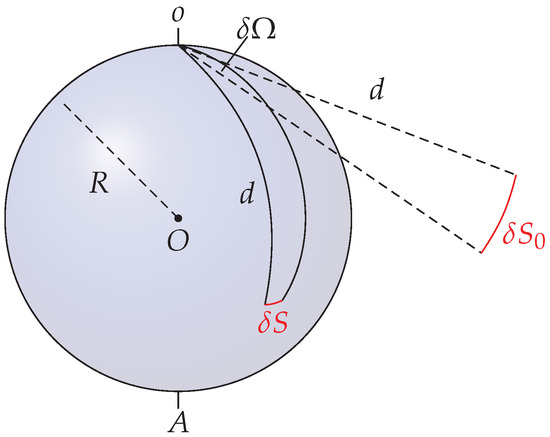
Figure 1. 2-dimensional representation of the distortion effect in the Einstein universe.

As seen in Figure 2a, the scaling factor decreases with the distance d until degeneration when the antipode A is reached, which corresponds to the distance $D=\pi R$. From the observer’s perspective, space seems to vanish at this point. An infinitesimally small source located at A appears stretched over the whole celestial vault, and the wavelengths of its photons are affected by this dilation. We get the following distance/redshift relation:

$$z_C={\displaystyle \frac{d}{Rsin\left(\frac{d}{R}\right)}}-1.$$

(8)

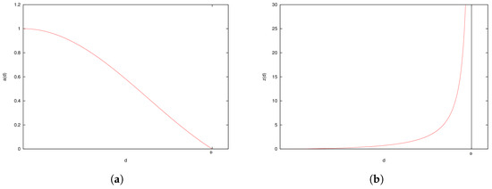
Figure 2. Evolution with proper distance of the scaling factor (a) and the redshift (b) in the Einstein universe.

• A graphical representation of Equation (8) is shown in Figure 2b. The derivative of the scaling factor with respect to d, that in big bang theories is interpreted as the rate of expansion of the universe, is given by

  $$a^{\prime }\left(d\right)={\displaystyle \frac{cos\left(\frac{d}{R}\right)}{d}}-{\displaystyle \frac{R}{d^2}}sin\left({\displaystyle \frac{d}{R}}\right).$$

  (9)

As seen in Figure 3, the variation of $a^{\prime }$ changes at a certain distance $d_0$. Observations of type Ia Supernovae have confirmed this behavior [22], and standard cosmological models attribute it to an acceleration of the expansion of the universe that started a few billions years ago.

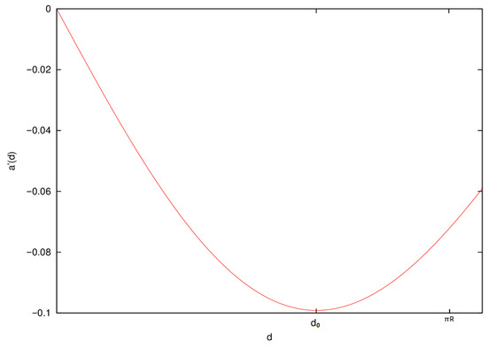
Figure 3. Evolution of the derivative of the scaling factor with proper distance.

4.2. Relations Between Different Distances

The proper distance d of celestial bodies is difficult to estimate directly from observations6. Instead, two redshift-independent methods are commonly used to assess their distances. Both require knowledge about the observed object. The luminosity distance $d_L$ is computed by comparing the flux of incoming light with the known luminosity of the source. The estimation of the angular diameter distance $d_A$ requires for its part knowledge about the size of the observed object.

$d_L$ is defined implicitly in the relation:

$$F_{obs}={\displaystyle \frac{L}{4\pi d_L^2}}.$$

(10)

Here, $F_{obs}$ is the flux measured by the observer and L is the known luminosity of the object in its local referential. Let us consider an object situated at proper distance d from the observer, that emits n photons of energy $h\nu$ per unit of surface per unit of time, where all these quantities are expressed in the natural referential of the object. In $R_{obs}$, the situation is equivalent to the following: in a flat universe, an object at proper distance d is emitting n photons of energy $h\nu /(z+1)$ per ${(z+1)}^2$ units of surface per $(z+1)$ units of time. Therefore, the luminosity of the object for the observer is

$$L_{obs}=L/{(z+1)}^4.$$

In the Euclidean space $R_{obs}$, the measured flux follows the inverse square law, so that

$$F_{obs}={\displaystyle \frac{L_{obs}}{4\pi d^2}}={\displaystyle \frac{L}{4\pi d^2{(z+1)}^4}}.$$

(11)

Combining (10) and (11), we get that

$$d_L=d{(z+1)}^2.$$

(12)

In a space of spherical geometry, the angular diameter distance $d_A$ is for its part given by

$$d_A=Rsin\left({\displaystyle \frac{d}{R}}\right)={\displaystyle \frac{d}{z+1}},$$

(13)

so that

$$d_L=d_A{(z+1)}^3.$$

(14)

Note that the Etherington-Ellis reciprocity relation does not hold in this theory. Indeed, the fundamental symmetry between source and observer on which this result rests is broken by the construction of the representation referential. In particular, in the representation referential, the area covered by a bundle of light rays emitted from the source and arriving at the observer is no longer equal to the area covered by a bundle of rays emitted from the observer and reaching the source. We will see in the following section that our theory reproduces the key features of Supernovae Hubble diagrams and angular diameter distance/redshift diagrams.

4.3. Comparisons with Observations

In Figure 4, we compare the distance law given by Equations (8) and (12) with Type Ia supernova observations from the Pantheon catalog [23]. A simple ${\chi }^2$ comparison was performed on the subset of distant supernovae with $z>0.5$ (216 data points), yielding an indicative curvature radius of $R=2.744$ Gly, corresponding to an antipodal region located at a proper distance $D=R\pi =8.621$ Gly from the observer. The resulting curve reproduces the overall trend of the observed luminosity distance/redshift relation, particularly at high redshift. At low redshift, deviations are more pronounced and may be partly attributed to peculiar velocities and calibration uncertainties that dominate the error budget in this regime.

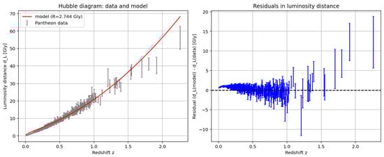
Figure 4. Best fit for the distant galaxies dataset (left) obtained for $R=2.744$ Gly and associated residuals (right).

It should also be emphasized that the Pantheon catalog is not a model-independent dataset: its distance moduli are derived under the assumption of an expanding cosmology, through the use of cosmology-dependent K-corrections and light-curve fitting procedures [24]. The present comparison should therefore not be regarded as a quantitative test of the proposed distance law, but rather as an illustrative exercise showing that the model can qualitatively reproduce the observed redshift/distance trend under such conditions. A rigorous evaluation would require reanalysis of raw photometric data without cosmological priors, which are not publicly available.

In Figure 5, the theoretical curve of the angular diameter distance relation, derived from Equations (8) and (13) with $R=2.744$ Gly, is shown together with observational estimates obtained from hydrostatic equilibrium analyses in [25]. Due to the large uncertainties and model dependencies affecting these measurements, no formal fit was performed, but the general behavior remains consistent within the data.

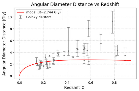
Figure 5. Comparison between the theoretical curve for $R=2.744$ Gly and observational data for the angular diameter distance.

Figure 4 and Figure 5 illustrate the theoretical predictions of the luminosity distance and angular diameter distance relations. Both curves reproduce the overall trends observed in the respective datasets. However, the uncertainties in the angular diameter distance measurements remain too large to allow a precise verification of the ${(z+1)}^3$ scaling predicted by Equation (14). This relation differs from the standard Etherington–Ellis reciprocity law, which scales as ${(z+1)}^2$, although both expressions are nearly indistinguishable at low redshift, where ${(z+1)}^2$ and ${(z+1)}^3$ differ only slightly. Only a few model-independent tests of the reciprocity relation have been carried out [26,27], and they are limited to this low-redshift regime, where the two laws are observationally difficult to distinguish. One such test has reported deviations from the ${(1+z)}^2$ behavior [26]. Accordingly, the present comparisons should be viewed as qualitative illustrations of the model’s behavior rather than quantitative tests. A more conclusive evaluation will require model-independent distance measurements and a consistent treatment of large-scale inhomogeneities, which could significantly affect the inferred redshift values in our framework.

Finally, we note that the model relies on a single geometric parameter, the curvature radius R, to reproduce the main features of the distance–redshift relation. This contrasts with the several free parameters required in the standard $\mathrm{\Lambda }$CDM framework. The model’s simplicity is appealing but requires confirmation through consistent observational tests.

5. Cosmic Microwave Background

The Cosmic Microwave Background is a radiation detectable at all locations in the universe which is extremely regular in all directions in space, although admitting small anisotropies distributed with privileged angle scales [7]. Its observed spectrum is one of a black body that has a maximum of emission at $\mathrm{\Lambda }\approx 2$ mm. The existence and the characteristics of the CMB are thought to be strong evidence for a big bang scenario since it fits very well the predictions of $\mathrm{\Lambda }$CDM [28], although several anomalies have been pointed out [29]. This section aims to show that the presented theory is also compatible with these observations.

5.1. Over the Horizon

Until here, our analysis has been limited to proper distances smaller than the maximal geodesic distance $D=\pi R$. Although it corresponds to an apparent horizon, one can perceive in this model (ghost) images of objects at distances larger than D. We then extend our definition of distance d to objects over this horizon, so that it corresponds to the length of the trajectory of a photon from the object to the observer. Applying the arguments developed in the previous sections, we get that the scaling factor is given by:

$$a\left(d\right)=\left|{\displaystyle \frac{Rsin\left(\frac{d}{R}\right)}{d}}\right|.$$

The observed redshift is then:

$$z\left(d\right)=\left|{\displaystyle \frac{d}{Rsin\left(\frac{d}{R}\right)}}\right|-1.$$

5.2. Thermal Radiation

In the context of a static universe, we cannot explain the CMB by photons emitted by a hot plasma in a primordial state of the universe. These photons must emanate from standard cosmological objects (mostly galaxies). By looking at Figure 6, we can characterise two classes of sources that produce highly redshifted light, which could contribute to the CMB:

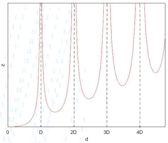
Figure 6. Evolution of the redshift with distance.

1.

Very old objects whose radiation has traveled around the universe many times before arriving at us, at a huge distance from us. This type of source will be referred to as class 1.

2.

Objects that emitted the perceived light in the region of one pole of the 3-sphere (our current position or its antipode), whose distance is near a multiple of D. This type of object will be referred to as class 2.

We assume that class-2 objects contribute negligibly to the microwave background compared to the dominant type-1 sources. The ancient light from these distant objects, strongly redshifted, has undergone repeated scattering, absorption, and re-emission by dust. In a fully symmetric, homogeneous, isotropic, and static Universe, such photons must form a spatially uniform radiation field. Reprocessing in a statistically homogeneous and isotropic medium enforces translation invariance and drives the field toward thermal equilibrium. Consequently, the resulting spectrum is necessarily of blackbody form, with a low characteristic temperature $T_{CMB}$ set by the redshifted wavelengths of class-1 emissions. In principle, the value of $T_{CMB}$ could be derived without direct measurement of the CMB, by analyzing the emission and absorption properties of the cosmic matter content together with the distribution and characteristics of radiation sources.

5.3. Anisotropies

In the current concordance model, the CMB anisotropies are explained by Baryonic Acoustic Oscillations of the dense primordial plasma. However, a recent study brings nuance to this explanation and suggests that up to the entirety of these fluctuations can be explained by galactic emissions reprocessed by dust assuming $\mathrm{\Lambda }$CDM [30]. We now show that these irregularities can also be explained by galactic emissions reprocessed by dust in the present theory7. More particularly, they are consistent with the presence of type 2 objects (mostly galaxies) in the high-redshift pole regions, which leave some characteristic prints on the CMB. Each pole contributes to one level of anisotropy and explains the peaks in the angular power spectrum of the CMB temperature anisotropy. To formalise this idea, we first assume that the emission spectrum of a galaxy is reduced to its strongest wavelength ${\lambda }_0$, which we assume to be the same for every galaxy. We also assume that the power spectrum of the CMB is centered around its strongest wavelength $\mathrm{\Lambda }$. These strong restrictions should still provide a decent estimate of the location of the peaks in the power spectrum.

To add to the regular background of wavelength $\mathrm{\Lambda }$, the received light must also have observed wavelength $\mathrm{\Lambda }$, so the source must be at a distance d that satisfies the equation

$${\displaystyle \frac{{\lambda }_0}{a\left(d\right)}}=\mathrm{\Lambda },$$

that is:

$${\displaystyle \frac{{\lambda }_0}{\mathrm{\Lambda }}}d=\mid Rsin\left({\displaystyle \frac{d}{R}}\right)\mid .$$

(15)

The solutions of the above equation are typically close to the pole at distance $k\pi R$ from us, which we call the pole k. For each k, there are two associated solutions, $d_k$ and $d_k^{\prime }$, which correspond to distances from the pole k of $l_k=k\pi R-d_k$ and $l_k^{\prime }=d_k^{\prime }-k\pi R$. Replacing in Equation (15), we obtain:

$$\left\{\begin{array}{c}{\displaystyle \frac{{\lambda }_0}{\mathrm{\Lambda }}}(k\pi R-l_k)=\mid Rsin({\displaystyle \frac{l_k}{R}})\mid ,\hfill \\ {\displaystyle \frac{{\lambda }_0}{\Lambda }}(k\pi R+l_k^{\prime })=\mid Rsin({\displaystyle \frac{l_k^{\prime }}{R}})\mid .\hfill \end{array}\right.$$

(16)

As $l_k$ and $l_k^{\prime }$ are typically small compared to R, we get

$$\left\{\begin{array}{c}{\displaystyle \frac{{\lambda }_0}{\mathrm{\Lambda }}}(k\pi R-l_k)\approx l_k\hfill \\ {\displaystyle \frac{{\lambda }_0}{\mathrm{\Lambda }}}(k\pi R+l_k^{\prime })\approx l_k^{\prime },\hfill \end{array}\right.$$

(17)

so that

$$\left\{\begin{array}{c}{l}_k={\displaystyle \frac{k\pi R}{\frac{\mathrm{\Lambda }}{{\lambda }_0}+1}}\hfill \\ l_k^{\prime }={\displaystyle \frac{k\pi R}{\frac{\mathrm{\Lambda }}{{\lambda }_0}-1}}.\hfill \end{array}\right.$$

(18)

Since ${\displaystyle \frac{\mathrm{\Lambda }}{{\lambda }_0}}$ has a big order of magnitude (≈${10}^4$), $l_k$ and $l_k^{\prime }$ correspond roughly to the same distance to the pole k, that we call again $l_k$:

$$l_k={\displaystyle \frac{{\lambda }_{0}k\pi R}{\mathrm{\Lambda }}}$$

(19)

Now that we have found the typical distance of these galaxies to the pole k, we can estimate the contribution of the pole k to the anisotropy power spectrum, by computing the number of galaxies near the pole k that will imprint their mark on the CMB. To constitute an anisotropy, their image must have an observed wavelength between $\mathrm{\Lambda }-\epsilon$ and $\mathrm{\Lambda }+\epsilon$, being $\epsilon$ of the order of the width of the CMB spectrum.

From Equation (19), these galaxies are at a distance from the pole k between

$$l_1^k={\displaystyle \frac{{\lambda }_{0}k\pi R}{\mathrm{\Lambda }+\epsilon }}$$

and

$$l_2^k={\displaystyle \frac{{\lambda }_{0}k\pi R}{\mathrm{\Lambda }-\epsilon }}.$$

Let $\rho$ be the mean density of galaxies in the universe (we assume a homogeneous distribution of galaxies). In $S^3$, the volume of space between $l_1^k$ and $l_2^k$ is given by

$$\begin{array}{cc}\hfill V& =\pi R^2(2l_2^k-2l_1^k+Rsin({\displaystyle \frac{2l_2^k}{R}})-Rsin({\displaystyle \frac{2l_1^k}{R}}))\hfill \\ \hfill & \approx 4\pi R^2(l_2^k-l_1^k),\hfill \end{array}$$

(20)

so that the number of galaxies at distances between $l_1^k$ and $l_2^k$ to the pole k is

$$\begin{array}{cc}\hfill N& =k\pi \rho 4\pi R^3{\lambda }_0({\displaystyle \frac{1}{\mathrm{\Lambda }-\epsilon }}-{\displaystyle \frac{1}{\mathrm{\Lambda }+\epsilon }})\hfill \\ \hfill & \approx {\displaystyle \frac{8{\pi }^2{R}^3\rho k{\lambda }_0ϵ}{{\mathrm{\Lambda }}^2}}.\hfill \end{array}$$

(21)

The number of galaxies associated with the pole k whose images are imprinted in the CMB is then $2N$, since the galaxies at distance $d_k^{\prime }$ also leave the same characteristic prints. If we assume equidistribution of the galaxies and independence between the images of the galaxies at distances $d_k$ and $d_k^{\prime }$, these galaxies are equally spaced on the celestial vault and their number corresponds to the multipole moment $P_k$ for which there is a peak in the power spectrum:

$$P_k={\displaystyle \frac{16{\pi }^2{R}^3\rho {\lambda }_0\epsilon k}{{\mathrm{\Lambda }}^2}}=C_{\epsilon }k.$$

(22)

Equation (22) shows a linear relation between $P_k$ and k. We also predict that the strength of these peaks decreases with k, mostly due to extinction effects.

Overall, these results are compatible with the measurements of the Planck collaboration [28], although a more detailed analysis of the matter is needed. We have made some approximations in our computations and quite strong restrictions to arrive at this result. In reality, the spectra of both galaxies and CMB are composed of a large band of wavelengths. Moreover, the density of galaxies $\rho$ and their precise distribution may differ for the different pole regions, in particular, due to the lacunary structure of the large-scale distribution of matter in the universe. We acknowledge that a full treatment of the CMB spectra is beyond the present scope, and we plan to address this limitation in future work.

6. Conclusions and Comments

We have proposed a novel formalism which rests on few fundamental assumptions concerning observations in curved spacetimes. This model turns out to be consistent with various key cosmological observations, such as redshift-distance diagrams and the CMB, while clearing away questions raised by the existence of an initial space-time singularity. Furthermore, the absence of a chronological history of the Universe within this model explains the presence of coherent galactic structures in the high-redshift universe, recently detected by the James Webb Space Telescope.

More complete and model-independent data-based studies are still required to support this theory. In particular, a careful analysis of the CMB characteristics in the present context needs to be performed. Several complementary predictions could be verified experimentally in the short and longer run. For instance, we predict double images of galaxies near the antipodal region. Our framework could also explain the anomalous redshifts detected in diverse large galactic structures. As it is more difficult to check at our temporal scale, the temperature of the CMB should not vary in time, and its anisotropies should evolve according to the characteristic dynamics of galaxies. This model also predicts the existence of a gravitational wave background, whose origin is analogous to that of the CMB.

As in quantum physics, our formalism introduces a duality between a more fundamental level of reality and its manifestation to the observer. In both contexts, the act of observation consists in projecting underlying structures onto a representational referential where they materialise into more familiar physical entities. Notably, the linear structure of $R_{obs}$ offers a fixed background consistent with the axioms of quantum mechanics, which could provide a unified framework for a theory of quantum gravity.

Appendix A.1. No Cosmological Redshift in the Newtonian Limit

We show here that our model predicts no redshift other than the gravitational one in the Newtonian limit. Consider an observer $\mathcal{O}$ subject to a uniform gravitational field $-g$ in the vertical direction z. By the Equivalence Principle, this situation is equivalent to a uniform vertical acceleration g as seen by a free falling observer. We compute the redshift $z_C$ of a photon emanating from a source s at proper distance $d=ct$ from $\mathcal{O}$. To follow the procedure described in Section 2, a light beam of infinitesimal solid angle $\delta \mathrm{\Omega }$ is sent from $\mathcal{O}$ in the direction of s. Locally at $\mathcal{O}$, it forms a cone of semi apex angle $\delta \mathrm{\omega }=\sqrt{{\displaystyle \frac{\mathrm{\delta }\mathrm{\Omega }}{\pi }}}$. The surface $\delta S$ intercepted by the bundle at s is delimited by an ellipse with semi axes of lengths $l_{\Vert }$ and $l_{\perp }$, where $l_{\Vert }$ represents the semi-axis contained in the plane $xz$, x being the axis chosen such that the $xz$ plane contains both the source and the observer. We denote by $l_{\perp }$ the length of the semi-axis of the ellipse lying in the direction y, orthogonal to $xz$. Let $\mathrm{\Theta }$ be the angle between the x axis and the null geodesic connecting $\mathcal{O}$ to s. The positions $\left(x_{-}\left(t\right),y_{-}\left(t\right),z_{-}\left(t\right)\right)$ and $\left(x_{+}\left(t\right),y_{+}\left(t\right),z_{+}\left(t\right)\right)$ of the outermost photons forming the boundary of the intersection of the bundle with the $xz$ plane are given by:

$$\begin{array}{cc}\hfill & x_{\pm }\left(t\right)=ccos(\mathrm{\Theta }\pm \delta \omega )t\hfill \end{array}$$

(A1)

$$\begin{array}{cc}\hfill & y_{\pm }\left(t\right)=0\hfill \end{array}$$

(A2)

$$\begin{array}{cc}\hfill & z_{\pm }\left(t\right)=-g{t}^2+csin(\mathrm{\Theta }\pm \delta \omega )t.\hfill \end{array}$$

(A3)

The length of the semi-axis $l_{\Vert }$ is then given by:

$$\begin{array}{cc}\hfill l_{\Vert }& ={\displaystyle \frac{1}{2}}\sqrt{{(x_{+}\left(t\right)-x_{-}\left(t\right))}^2+{(z_{+}\left(t\right)-z_{-}\left(t\right))}^2}\hfill \end{array}$$

(A4)

$$\begin{array}{cc}\hfill & ={\displaystyle \frac{ct}{2}}\sqrt{[{(cos(\mathrm{\Theta }+\delta \omega )-cos(\mathrm{\Theta }-\delta \omega )]}^2+{[sin(\mathrm{\Theta }+\delta \omega )-sin(\mathrm{\Theta }-\delta \omega )]}^2}\hfill \end{array}$$

(A5)

$$\begin{array}{cc}\hfill & =ct\delta \omega \sqrt{{sin}^2\mathrm{\Theta }+{cos}^2\mathrm{\Theta }}\hfill \end{array}$$

(A6)

$$\begin{array}{cc}\hfill & =ct\sqrt{{\displaystyle \frac{\delta \mathrm{\Omega }}{\pi }}}.\hfill \end{array}$$

(A7)

Similarly, we can show that

$$l_{\perp }=ct\delta \omega =ct\sqrt{{\displaystyle \frac{\delta \mathrm{\Omega }}{\pi }}}.$$

Therefore, the interior of the ellipse intercepted by the bundle has area:

$$\begin{array}{cc}\hfill \delta S& =\pi l_{\Vert }{l}_{\perp }=c^2{t}^2\delta \mathrm{\Omega },\hfill \end{array}$$

(A8)

which also equals $\delta S_{obs}$. We conclude that

$$\begin{array}{cc}\hfill z_C& =\sqrt{{\displaystyle \frac{\delta S_{obs}}{\delta S}}}-1=0.\hfill \end{array}$$

(A9)

Appendix A.2. Comments on Locality

We have stated general principles concerning the observation of distant objects in curved spacetimes. A natural question is whether the evolution of the observed wavelength of a photon ${\lambda }_{obs}$ along geodesics can be reinterpreted as originating from local physical processes. If so, there would exist a function f depending only on the local structure at the photon position such that for small $\epsilon$,

$${\lambda }_{obs}(d+\epsilon )=f({\lambda }_{obs}\left(d\right),\epsilon ).$$

(A10)

This is not the case since we have

$${\lambda }_{obs}(d+\epsilon )={\lambda }_{obs}\left(d\right)+{\lambda }_{em}{a}^{\prime }\left(d\right)\epsilon ,$$

(A11)

which depends strongly on both the wavelength at emission ${\lambda }_{em}$ and the distance d from the source. In this sense, the theory is, as quantum physics, non local.

However, if one takes the point of view of the observer and reasons in terms of the representation referential $R_{obs}$, the wavelength remains constant after emission and the theory is therefore trivially local. In this view, the principle of locality is attached to the observer’s representation of its environment and is not an intrinsic property of the underlying physical reality.

References

- Eddington, A.S. On the instability of Einstein’s spherical world. Mon. Not. R. Astron. Soc. 1930, 90, 668–678. [Google Scholar] [CrossRef]
- McCoy, C.D. Stability in Cosmology, from Einstein to Inflation. In Thinking About Space and Time; Springer International Publishing: Cham, Switzerlands, 2020; Volume 15. [Google Scholar]
- Hubble, E.P. A relation between distance and radial velocity among extra-galactic nebulae. Proc. Natl. Acad. Sci. USA 1929, 15, 168–173. [Google Scholar] [CrossRef]
- Nussbaumer, H. Einstein’s conversion from a static to an expanding universe. Eur. Phys. J. H 2014, 39, 37–62. [Google Scholar] [CrossRef]
- Lemaître, G. Un Univers homogène de masse constante et de rayon croissant rendant compte de la vitesse radiale des nébuleuses extra-galactiques. Ann. Soc. Sci. Brux. 1927, A47, 49–59. [Google Scholar]
- Einstein, A.; de Sitter, W. On the Relation between the Expansion and the Mean Density of the Universe. Proc. Natl. Acad. Sci. USA 1932, 18, 213–214. [Google Scholar] [CrossRef]
- Penzias, A.A.; Wilson, R.W. A Measurement of Excess Antenna Temperature at 4080 Mc/s. Astrophys. J. 1965, 142, 419–421. [Google Scholar] [CrossRef]
- Copeland, E.J.; Sami, M.; Tsujikawa, S. Dynamics of dark energy. Int. J. Mod. Phys. D 2006, 15, 1753–1935. [Google Scholar] [CrossRef]
- Zwicky, F. On the Red Shift of Spectral Lines through Interstellar Space. Proc. Natl. Acad. Sci. USA 1929, 15, 773–779. [Google Scholar] [CrossRef]
- Wright, E.L. Errors in Tired Light Cosmology. Available online: https://www.astro.ucla.edu/~wright/tiredlit.htm (accessed on 2 June 2021).
- Riess, A.G.; Casertano, S.; Yuan, W.; Macri, L.M.; Scolnic, D. Large Magellanic Cloud Cepheid Standards Provide a 1% Foundation for the Determination of the Hubble Constant and Stronger Evidence for Physics Beyond LambdaCDM. Astrophys. J. 2019, 876, 85. [Google Scholar] [CrossRef]
- Valentino, E.D.; Melchiorri, A.; Silk, J. Planck evidence for a closed Universe and a possible crisis for cosmology. Nat. Astron. 2020, 4, 196–203. [Google Scholar] [CrossRef]
- Bohm, D. Wholeness and the Implicate Order; Routledge: London, UK, 1980. [Google Scholar]
- Einstein, A. Zur Electrodynamik bewegter Koerper. Ann. Phys. 1905, 322, 891–921. [Google Scholar] [CrossRef]
- Perlick, V. Gravitational Lensing from a Spacetime Perspective. Living Rev. Relativ. 2024, 7, 9. [Google Scholar] [CrossRef] [PubMed]
- Goldhaber, G.; Deustua, S.; Gabi, S.; Groom, D.; Hook, I.; Kim, A.; Kim, M.; Lee, J.; Pain, R.; Pennypacker, C.; et al. Observation of cosmological time dilatation using type 1A Supernovae as clocks. In Thermonuclear Supernovae; Springer: Dordrecht, The Netherlands, 1997; Volume 486. [Google Scholar]
- Pound, R.V.; Rebka, G.A. Gravitational Red-Shift in Nuclear Resonance. Phys. Rev. Lett. 1959, 3, 439–441. [Google Scholar] [CrossRef]
- Hernández, J.G.; Rebolo, R.; Pasquini, L.; Curto, G.L.; Molaro, P.; Caffau, E.; Ludwig, H.-G.; Steffen, M.; Esposito, M.; Mascareno, A.S.; et al. The solar gravitational redshift from HARPS-LFC Moon spectra—A test of the general theory of relativity. Astron. Astrophys. 2020, 643, A146. [Google Scholar] [CrossRef]
- Arp, H.C. Anomalous redshifts. In Current Issues in Cosmology; Pecker, J.-C., Narlikar, J., Eds.; Cambridge University Press: Cambridge, UK, 2006; pp. 183–196. [Google Scholar]
- Ratcliffe, H. Anomalous Redshift Data and the Myth of Cosmological Distance. J. Cosmol. 2010, 4, 693–718. [Google Scholar]
- Einstein, A. Kosmologische Betrachtungen zur Allgemeinen Relativitatstheorie. In Das Relativitätsprinzip. Fortschritte der Mathematischen Wissenschaften in Monographien; Vieweg+Teubner Verlag: Wiesbaden, Germany, 1919; Volume 7, p. 232. [Google Scholar]
- Friedman, J.A.; Turner, M.S.; Huterer, D. Dark Energy and the Accelerating Universe. Annu. Rev. Astron. Astrophys. 2008, 46, 385–432. [Google Scholar] [CrossRef]
- Scolnic, D.M.; Jones, D.O.; Rest, A.; Pan, Y.C.; Chornock, R.; Foley, R.J.; Huber, M.E.; Kessler, R.; Narayan, G.; Riess, A.G.; et al. The Complete Light-curve Sample of Spectroscopically Confirmed SNe Ia from Pan-STARRS1 and Cosmological Constraints from the Combined Pantheon Sample. Astrophys. J. 2018, 859, 101. [Google Scholar] [CrossRef]
- Scolnic, D.M.; Jones, D.O.; Rest, A.; Pan, Y.C.; Chornock, R.; Foley, R.J.; Huber, M.E.; Kessler, R.; Narayan, G.; Riess, A.G.; et al. On the dependence of type Ia SNe luminosities on the metallicity of their host galaxy. Astrophys. J. 2016, 818, 19. [Google Scholar] [CrossRef]
- Bonamente, M.; Joy, M.K.; LaRoque, S.J.; Carlstrom, J.E.; Reese, E.D.; Dawson, K.S. Determination of the cosmic distance scale from Sunyaev-Zel’dovich effect and Chandra X-ray measurements of high red-shift galaxy clusters. Astrophys. J. 2006, 647, 25. [Google Scholar] [CrossRef]
- Holanda, R.F.L.; Lima, J.A.S.; Ribeiro, M.B. Testing the distance–duality relation with galaxy clusters ans Type Ia Supernovae. Astrophys. J. Lett. 2010, 722, 233–237. [Google Scholar] [CrossRef]
- Hu, L.H.; Wu, P.X.; Yu, H.W. The distance duality relation test from the ACT cluster and type Ia supernova data. Res. Astron. Astrophys. 2016, 16, 016. [Google Scholar] [CrossRef]
- Planck Collaboration. Planck 2015 results. XI. CMB power spectra, likelihoods, and robustness of parameters. Astron. Astrophys. 2016, 594, A11. [Google Scholar] [CrossRef]
- Schwarz, D.J.; Copi, C.J.; Huterer, D.; Starkman, G.D. CMB anomalies after Planck. Class. Quantum Grav. 2016, 33, 184001. [Google Scholar] [CrossRef]
- Gjergo, E.; Kroupa, P. The impact of early massive galaxy formation on the cosmic microwave background. Nucl. Phys. B Spec. Issue Clarifying Misconceptions 2025, 1017, 116931. [Google Scholar] [CrossRef]
Disclaimer/Publisher’s Note: The statements, opinions and data contained in all publications are solely those of the individual author(s) and contributor(s) and not of MDPI and/or the editor(s). MDPI and/or the editor(s) disclaim responsibility for any injury to people or property resulting from any ideas, methods, instructions or products referred to in the content. |
© 2025 by the author. Licensee MDPI, Basel, Switzerland. This article is an open access article distributed under the terms and conditions of the Creative Commons Attribution (CC BY) license (https://creativecommons.org/licenses/by/4.0/).