Abstract
Using the projection evolution (PEv) approach, time can be included in quantum mechanics as an observable. Having the time operator, it is possible to explore the temporal structure of various quantum events. In the present paper, we discuss the possibility of constructing a quantum clock which advances in time during its quantum evolution, in each step having some probability to localize itself on the time axis in the new position. We propose a working two-state model as the simplest example of such a clock.
PACS:
03.65.-w; 03.65.Ca; 03.65.Ta
1. Introduction
Time is one of the most important features of our physical world. Its measurement is a fundamental procedure, and not only in physics. At every step of technical development there are projects of investigation leading to the construction of better and better clocks which are able to measure extremely small time intervals [1,2,3,4].
In book [5], three types of time are discussed: time as a parameter, dynamical time, and time as a quantum observable. The most consistent with quantum mechanics is the last concept, i.e., time as a quantum observable, considered on the same footing as the other position operators. In physics, especially in the quantum regime, one requires more and more precise measurements of time to better understand and predict the evolution of such systems. On the other hand, to measure very short time intervals one needs to construct a clock which, in fact, is a specific quantum system working according to quantum rules and, in addition, is often (weakly) coupled to the measured system.
For many years time was treated in physics as a universal parameter enumerating the evolution of physical systems. Special and general relativity changed this notion substantially. In quantum mechanics, however, especially after the publication of the Pauli theorem [6,7], time is still considered as an evolution parameter.
Overviews of the role of time in quantum mechanics can be found, among others, in [8,9,10,11,12,13,14,15,16,17,18,19,20,21,22,23,24,25,26,27,28,29,30,31,32,33,34,35,36,37,38,39,40,41].
A nice discussion about both the early and more recent works concerning quantum time and quantum clocks can be found in the review paper [42]. In the model of Wigner and Salecker [43], time has the form of a parameter with discrete values, , where , and is the time unit. Peres [44] recognized in the full Hamiltonian its temporal part , given by . Here, , , is a discrete parameter and served a similar role as the time of Wigner and Salecker. The Page and Wootters model [45], on the other hand, contains two times: the internal time of the clock, and the external macroscopic time. The clock is represented by the evolution of a quantum observable. The outcomes of the measurements of this observable serve as indicators that time passes. In other words, the internal time in the Page–Wootters model is a quantum observable, while the external time is defined by the classical readouts of this observable through the measurement process. In our model, we call such a system the `clock’ and its subsystem responsible for the measurements the `interface’. A few problems with the Page–Wootters model were pointed out, starting with the observation that their clock was not able to make more than one tick. Another objection was that in order to use conditional probability in their calculations, a preferred time variable is needed, and there is no procedure to make this choice. More details can be found in the review [42].
The authors of [42] extend the Page–Wootters model using the clock Hamiltonian , and conditioning the reference clock time to time t. The temporal part of the global wave function of the Universe is then given by the projection onto the state associated with time t as follows:
Finally, the time eigenstates are constructed as Fourier transforms of the energy eigenstates. Further discussion involves, among other topics, the problem of relating the proper time to the dynamics generated by the quantum clock, as well as the problem of the flow of time, i.e., the translation of the system along the time axis.
The main problem of the models described above is that in order to build a consistent model of a quantum clock, time must be included in the theory as a quantum observable. A time operator, therefore, is needed, acting in a similar way on the wavefunction as the position operators. The wavefunction itself must be dependent on all four coordinates of spacetime, where time appears on an equal footing with the position variables. This approach solves the problem of a preferred time variable, as well as the Hamiltonian constraint given by the Wheeler–DeWitt equation , and the problem of how to describe the flow of time.
In this paper, we treat time as a component of a composite quantum observable of the spacetime position. To be consistent, we use the projection evolution model (PEv),the most recent version of which can be found in [46,47]. These references also present a more extended introduction to the problem and the corresponding bibliography.
According to the PEv approach, quantum time and space positions should be considered on the same footing. However, one needs to realize that we have direct access to the space position observable but only indirect access to the time position observable on the time axis. The latter requires special measuring devices called clocks. A proper clock definition is vital for investigating the structure of the real spacetime.
2. Projection Evolution
In a more general approach, the evolution of quantum states is described by the so-called quantum operations, which transform one quantum state into another. These can be viewed as the state changes happening at some spacetime points and respecting the probability distribution of the outcome [48,49,50].
One of the inherent quantum properties is the localization in spacetime. The projection evolution (PEv) formalism used in this paper allows the quantum spacetime position operators to be introduce and the spacetime position of any quantum object to be determined.
In order to model physical processes, one needs to localize the states and transitions in spacetime; therefore, time and positions must be included as variables of the quantum states. The PEv model contains the traditional Schrödinger evolution described in spacetime but also incorporates other evolution equations like the ones of Klein–Gordon, Dirac, and others.
Refs. [46,47] contain all the details of the PEv model and an extensive bibliography on the topic.
For readers’ convenience we summarize the main points of the PEv approach.
The main assumption of the PEv evolution model is the changes principle, which states that:
The evolution of a system is a random process caused by spontaneous changes in the Universe. These spontaneous changes are primary processes in the Universe.
In this approach, the changes in the quantum-state space happen according to a probability distribution which is dictated by the properties of the Universe and its subsystems. A very important attribute of our Universe is the spacetime itself, which should emerge from the quantum-state space. In this article, we consider the flat spacetime.
Every single step of the evolution describes the state of a physical subsystem (possibly the Universe as a whole) in this state space. It means that the evolution is not driven by time, which is a part of the system’s description at a given evolution step, but it is driven by an extra parameter . This parameter is not time; it belongs to a linearly ordered set with no additional structure required.
In the following, we are using , which can be represented by integers . This allows quantum events to be ordered and allows for the notion of the predecessor and the successor in any set of physical events. As a consequence, one may expect the existence of a kind of pseudo-causality based on the ordering of the quantum events, which leads to the causality principle in the case of macroscopic physical systems. An additional, very important feature of the PEv approach is that this idea does not need the spacetime as the background, it is background-free. The spacetime is “generated” by the spacetime position observable.
In the projection evolution formalism, we propose using the generalized form of the Lüders [51] type of the projection postulate as an evolution principle. This allows, as a special case, the standard unitary evolution to be reproduced, represented by relativistic and non-relativistic evolution equations.
In the following, we introduce the evolution operators which can characterize a given physical system. They are formally responsible for quantum evolution of this object. In this paper, we are using the evolution operators represented by an orthogonal resolution of unity:
where denotes the unit operator and represents a set of quantum numbers describing quantum states. Different alternatives representing random choices of quantum states are described by different sets of quantum numbers . Such types of operators are able to describe a wide class of physical systems.
Assume now, that the vector represents a given quantum state at the evolution step , where .
The changes principle implies that there exists in the Universe a physical mechanism, we call it the chooser, which chooses randomly the next state of the system from the set of states determined by the projection postulates:
where the global phase can be chosen arbitrarily and denotes the norm of the vector v.
In other words, Equation (3) determines the set of allowed states to which a physical system can randomly evolve from the state . To fully describe this stochastic process, one needs to know the probability distribution for obtaining a given state in the next step of the evolution. It is given by
It is also useful to introduce a tool which facilitates the construction of the evolution operators in terms of the projection operators. We have found that the required evolution operators can be obtained from some operators , which we call generators of the projection evolution [46].
For a given evolution step , the projection evolution generator is defined as a self-adjoint operator whose spectral decomposition gives the orthogonal resolution of unity representing the required set of the evolution operators.
For example, assuming a discrete spectrum of an evolution generator , the spectral theorem gives the following relation between and the evolution operators : . Where are the eigenvalues of . In the case of a continuous spectrum, one needs to use the integral form of the spectral theorem.
The evolution generators allow the already known quantum operators to be used to generate the appropriate evolution operators .
Using the projection evolution model allows the construction of the quantum clock in a consistent way. In our formulation:
- Time t is a quantum observable—the time operator allows the quantum state to be localized on the time axis in the same way as the position operators localize the state in space;
- The operator represents the momentum of the system along the time axis; the sign of the eigenvalues of determines the direction of the “the arrow of time”;
- The clock is a quantum system for which the mean value of the time operator changes;
- A subsystem of the clock, we call it the interface, periodically determines and localizes the clock on the time axis, which is interpreted as the classical time flow.
3. Quantum Clock in the Structureless Flat Spacetime
In particle, atomic, molecular, and some other branches of physics, one expects that the clock, as a measuring device, is weakly coupled to the measured physical system and to its environment. The weak coupling assures that the measurement does not disturb the measured system. In the present paper, without the loss of generality, we treat the clock as being completely decoupled from the measured system.
However, it is only an approximation because the clock is, in fact, a part of this system. In models in which time is a quantum observable, it should be considered as a part of an observable describing the position in spacetime. The position in quantum spacetime is, in turn, one of the attributes of physical matter.
In this paper, we consider the simplest, approximate model which leads to the spacetime based on the quantum-state space, i.e., the Hilbert space of square integrable functions with the scalar product (note the integration over time) [46,47].
In a fixed coordinate frame, a possible realization of the spacetime position operator can be given by the four-vector operator , where .
We understand the term four-vector as a four-component object which transforms with respect to a given group of the spacetime transformations. In our case, we think about two groups: either the Galilean or the Lorentz group. This means that using the same denotations we may consider either a non-relativistic or relativistic four-dimensional flat spacetime.
The canonically conjugated observable is the four-momentum operator . Because time is a quantum observable , the temporal momentum is the corresponding counterpart. By analogy to the space components of the momentum operator one can think about as an observable representing the measure of motion in the temporal dimension. The sign of describes the arrow of time. The temporal momentum can be measured using different equations of motion, which relate it to the spatial and other properties of the system. For example, the Schrödinger equation , where the variables represent some additional degrees of freedom of the quantum system, relates to the Hamiltonian . One can say the same about the Klein–Gordon, Dirac, and other equations of motion.
In principle, we need some kind of “detectors” measuring positions in spacetime. They can be represented by POV measures [52]. In the ideal case, this measure is represented by a sharp observable given by the projection operators , where the vectors are eigenstates of the position operators .
In such models, we come across the (1+3)-D position measurement. There is no problem with performing the 3D spatial measurement; however, we do not have devices which allow us to see the whole time axis, i.e., the past, present, and the future. It seems that our material world is, in most cases, rather well localized in time, and that only a narrow temporal window moving along the time axis is available for us in the experiments. From this perspective, a clock has to be a part of the quantum system, well localized in time, possibly coupled to other physical subsystems. Having a reference clock, one can construct other types of clocks as devices synchronized with this clock. This procedure allows the notion of “external time” to be introduced; however, only for systems which are well decoupled from the reference clock.
We define a quantum reference clock as a kind of device localized on the time axis and moving with a fixed sign of the average temporal momentum in spacetime. The sign is conventional but it defines the arrow of time. The clock localizing itself in a time interval (temporal window) shows us, usually indirectly by some kind of an interface (measurement), its position in time. This means that the clock consists of two subsystems: the proper clock, evolving from one localization on the time axis to another; and the interface reading off the clock’s time position.
In the PEv model [47], the average spacetime localization of a physical system can change only with the change in the evolution parameter . In the following, we denote by , the evolution steps of the proper clock, and by , where , the evolution steps at which the clock interface reads its temporal position. This implies that a given quantum clock at the evolution step is represented by a set of clock states . The label represents a set of quantum numbers describing both the temporal and other properties of observables required for the construction of a quantum clock. For a good clock, the variance in the time operator
where
projects onto the subspaces of simultaneous events, should be small. More precisely, the variance should fulfill the following inequality:
where is a small number and denotes the clock resolution. The corresponding expectation value of the time operator within the clock states, , gives the expected temporal position of the proper clock, i.e., it gives a parameter t representing the classical time. In the ideal case, the clock states are eigenstates of the time operator, with the variance (7) being equal to 0.
In the projection evolution model [47], an important element is the construction of the evolution operators for the subsequent steps of the evolution . This means that we have to describe the following process: for the evolution step the proper clock is localized at some time , this position is read off by the interface at and the proper clock is moving to the next temporal position at .
In this paper, we propose a set of unitary operations, driven by a random variable , transforming the evolution generators, not states, from the previous to the next step of the evolution process:
where is a coupling constant. The temporal momentum operator and the self-adjoint reconfiguring operator commute, i.e., . The temporal momentum operator is responsible for the motion along the time axis. The values of the random variable are related to the internal processes of the clock and to the influence of the environment on the clock. This leads effectively to a movement of the clock along the time axis. Direction of the clock motion along the time axis is determined by the expectation value of the temporal momentum operator , calculated in the clock states. The reconfiguring operator changes some internal states of the clock and allows the required clock interface to be defined.
Let us denote by the evolution generator of the proper clock at the evolution step . The unitary transformations (8) form a two-parameter group, , where . This feature allows the evolution generator to be related to its initial form :
where , and are subsequent values of the random variable .
To construct the evolution operators from the evolution generator one needs to find its spectral decomposition. Assuming a discrete spectrum of the generator , one has to solve the following eigenequation:
where c represents the possible degeneration of the spectrum. The transformation property (9) implies that it is sufficient to solve the eigenequation (10) only for to obtain all solutions for every . If are eigenvectors of , the states
are eigenstates of . The eigenvalues are independent of n.
The distribution of should have a pronounced maximum very close to zero. (In this work we assume but the general condition is, that has a distribution around zero, asymmetric towards values. This will result in the net time flow in the positive direction of the time axis. We will discuss this problem in a subsequent paper.) This implies, that the next instant of classical time during the evolution should be very close to the previous one. The probability distribution for is a parameter of the clock. It seems that this distribution is strongly related to both the construction of the clock, and the structure of spacetime.
The second component of the clock is an interface allowing the clock to be read. The interface is, therefore, a measuring device and its full evolution operator has to contain the appropriate projection operators.
The projection evolution generators simplify the construction of the required evolution operators for a quantum reference clock. This method will be used in the next section.
3.1. The Proper Clock
For a given observer, quantum spacetime splits into time and 3D position space. In the following, to present the clock idea we choose a non-covariant description of a proper clock and its interface.
Because we treat time on the same footing as the other coordinates, one expects that every interaction , where are spacetime points, depends not only on the positions in space but also on positions in time [46]. One can say the same about the effective potentials . According to observations, in a wide range of its density, physical matter is well localized in time. This supports parametric time as a good approximation. On the other hand, which is even more important, this feature also suggests that the interaction in the temporal dimension has a very short range. In normal-density matter, the temporal parts of interactions among many particles lead to a temporal mean-field effective potential operator . One can find a similar effect in nuclear physics, where the mean-field approach to a short-range nuclear interaction is a good approximation.
In the following, we present a non-relativistic proper clock described by a modified Schrödinger type of quantum motion in the structureless flat spacetime [46]. Relativistic versions of the clock can be constructed in a similar way.
Following the discussion about the evolution generators described in [46], the initial projection evolution generator for a proper clock is postulated in the following form:
where the temporal momentum operator is , and the Hamiltonian acts on functions of the position variables and potentially on some intrinsic variables, i.e., it does not depend on time. The signs in front of the temporal part of the generator (12) are chosen to keep the coefficient positive. By analogy to the spatial kinetic term in the Hamiltonian , the term can be called the “temporal inertia”.
The proper clock is determined by the generator, which describes the physical system localized in time, and the Hamiltonian , which allows an appropriate interface to be built in its state space. The proper clock is localized on the time axis by the effective temporal potential operator .
Using the unitary operator (8) one obtains the evolution generator for any arbitrary evolution step :
where the potential localizing the clock in time is given by
The modified Hamiltonian has the following form:
According to the definition of the projection evolution generators we have to construct the spectral decomposition of . For this purpose one needs to look for the eigenfunctions of . In our case, we can find them by separating the variables,
where . The indices and indicate a possible degeneration of the solutions. In the following, we assume that the temporal functions represent the states which, on average, move in the positive direction of time. This means that the temporal functions are the states for which the expectation value of the temporal momentum operator,
is a positive number.
The functions denote the eigenvectors of the Hamiltonian ,
where represents the eigenvalues of .
The function solves the equation
while together with the exponential function it constitutes the full solution of the equation
This allows one to write the eigenequation for as
with given by Equation (16) and
where the function labeling the eigenvalues of fulfills the condition: .
Collecting the above partial solutions, the eigenstates of for a given evolution step are given by the vectors
where and .
The evolution operators generated by are the projections onto eigenspaces of the evolution generator,
The Kronecker-type function is defined as if , otherwise it is equal to 0. The sums will be substituted by some integrals in the case of a continuous spectrum.
3.2. The Clock Interface
To read the change in the internal state of the proper clock, we introduce the interface evolution operators denoted by , where describes an intermediate event between and . They form an orthogonal resolution of unity projecting onto eigenstates of the Hamiltonian , showing in which eigenstate of the clock actually is. Changes in the states of the Hamiltonian along the time axis represent the clock ticks. The clock interface should disturb neither the proper clock localization in time nor its movement along the time axis but it should show in which eigenstate of the Hamiltonian the proper clock is.
Let us denote an orthonormal basis in the state space. We obtain the required properties by assuming that
where is the unit operator in the time domain. The projection operators (25) are independent of , i.e., we keep the same interface for every evolution step.
3.3. The Clock
The evolution operators described above allow different reference clocks to be constructed using different forms of the operators: , and .
The clock starts from any arbitrary quantum state . The evolution operator prepares the initial state of the clock:
where represents, according to the PEv formalism, a randomly chosen eigenvalue of the evolution generator .
The state (26) is read by the interface
where represents a randomly chosen eigenvalue of the Hamiltonian . The simplest choice of the initial state is any eigenstate of the evolution generator (16),
Then, , where and .
To simplify the notation let us denote by the sequence of quantum numbers which gives a possible evolution path
The subsequent cycles of the clock are described by the following recurrence relations:
and
where the probabilities of choosing next states are given by (4), i.e., by the denominators of (29) and (30), respectively.
The action of the evolution operator on any function can be written as
where the expansion coefficients, taking into account (24) and (25), read
Because the functions and are orthonormal, the coefficient which normalizes Equation (31) can be expressed by the coefficients (32)
Using the coefficients , the clock state (30) can be rewritten as
The definition (32) and Equations (33) and (34) lead to the recurrence relation for the -coefficients:
Having the -coefficients, one can calculate the transition probability between the subsequent readings off the interface. The square of the normalization factor represents this probability:
In our model, the clock shifts subsequently on the time axis about the random variable . However, our knowledge about this shift is supplied only by the clock interface. It is important to calculate the expectation value of the time operator within the states corresponding to reading off the interface. For this purpose, let us denote by the average value of the time operator in the state (30), i.e., . Using (30) and the following matrix elements:
the required expectation value reads
The ideal clock should show the value , i.e., the place where the clock is localized on the time axis. The interface, however, is also a quantum device and acts randomly. There is, therefore, a finite probability that the proper clock moves to the next position on the time axis, but the interface does not change its state, i.e., the “hand of the clock” does not advance forward. This implies that for a good clock the second term in (38) should always be close to zero.
4. A Two-State Clock
As an example, we build a schematic clock for which there is no summation over , and in Equation (24).
This is often the case when both (18) and (19) have discrete non-degenerate spectra, which allows the evolution operators to be rewritten (24) in a simpler form:
We express the clock Hamiltonian describing the clock interface by making use of the spectral theorem:
The reconfiguration operator is taken in the following form:
This means that our clock interface is oscillating between two states, and , and the corresponding evolution operators, reading the actual state of the interface, are given by
The state of the proper clock and its interface at the evolution step is . To reach the next step of the evolution one needs to calculate
and
Because in Equations (29) and (30) the common multiplication factors in the nominators and denominators can be simplified, and overall phases are unimportant, the resulting clock states, after simplification of notation, are represented by the vectors
The clock states (45) and (46) allow the transition probability between the states representing two subsequent readings from the clock interface to be calculated. The probability of passing the evolution path
according to the expression (36) reads
Using relations (43) and (44), one can cast (47) in the form
For the reconfiguration operator (41), the -dependent part of the operator (8) is given by
where is the unit operator in the full state space, while acts in its two-dimensional subspace only. It follows that the scalar product reads
which allows the transition amplitudes to be calculated:
To register the time passing is equivalent for the clock to change the state from to or from 0 to 1, i.e., the clock “clicks”. Using Equation (48) and the appropriate amplitudes (51)–(58) gives the probabilities that the clock “clicks”, in the form
The probability of the opposite event, i.e., that the clock changes its state without the “click”, is .
The probability that the clock “clicks” exactly in the ℓth step is given by
The probability amplitude can be expressed as
The elementary step of movement along the time axis should be extremely small, i.e., the expectation value of , for every step k of the clock evolution. This implies that to a very good approximation, and one can write .
Let us calculate the average value of the time operator . It is given by
Since , we have
A good clock is characterized by the term (63) being as small as possible. If , this term vanishes. It follows, that after n steps of evolution, the localization of the clock on the time axis is close to .
In a similar way, one may obtain the average value of the temporal momentum operator,
Since , the condition implies that the second term in Equation (64) vanishes, which results in a constant arrow of time:
To estimate how long, on average, we have to wait until a “click” appears, we calculate the variance in ℓ. The normalized probability that a single “click” takes place at any of the steps, during an ℓ-step evolution, is given by
This results in the average ℓ,
and the average ,
Thus, the variance is given by
The probability Equation (66) is presented in Figure 1 as a function of the number of steps ℓ. We note that for higher probabilities p the number of required evolution steps ℓ decreases. The exact position of the maximum is given by the relation
which for gives , for is , and for drops to .
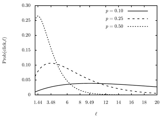
Figure 1.
The probability (66) of a single click during ℓ steps of the clock’s evolution. The values of p are , , and .
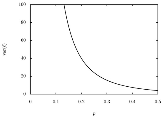
The variance in ℓ is presented in Figure 2. For the ideal case of , the average ℓ from Equation (67) is while the standard deviation reads . This gives the average number of the required evolution steps as .
5. Final Remarks
We expect that a quantum clock’s precision exceeds the precision reached by the currently used systems. For example, the time unit measured by an atomic clock is derived from the frequency of the photon emitted by an atom during its de-excitation. The stability of the chosen atomic transitions is so high that modern atomic clocks [1,2,3,4] achieve systematic uncertainty on the level of s, where this number is measured with respect to an external laboratory clock.
Since each evolution step advances the quantum clock on the time axis by and we are required to wait between 1 and 5 steps to register the click, the value of must be at least an order of magnitude smaller than to assure the already achieved precision.
In a more complicated case, in which has an uncertainty and its value is determined in each step of the evolution according to some probability distribution, we require the average to be small. In that case, one may take the statistics from as many evolution steps as needed, which will lower the value of and increase the clock’s accuracy to the required level.
We note also that every clock, even theoretically considered as a quantum system, is influenced by spacetime and physical fields. Observed changes in the clock can give information about the temporal structures of these objects. This is an open problem for future investigations.
Author Contributions
Both authors contributed equally to this manuscript. All authors have read and agreed to the published version of the manuscript.
Funding
This research received no external funding.
Data Availability Statement
No new data were created or analyzed in this study. Data sharing is not applicable to this article.
Conflicts of Interest
The authors declare no conflict of interest.
References
- Ludlow, A.; Hinkley, N.; Sherman, J.; Phillips, N.; Schioppo, M.; Lemke, N.; Beloy, K.; Pizzocaro, M.; Oates, C. An atomic clock with 10−18 instability. Science 2013, 341, 1215–1218. [Google Scholar]
- Ludlow, A.; Boyd, M.; Ye, J.; Peik, E.; Schmidt, P. Optical atomic clocks. Rev. Mod. Phys. 2015, 87, 637. [Google Scholar] [CrossRef]
- Huntemann, N.; Sanner, C.; Lipphardt, B.; Tamm, C.; Peik, E. Single-Ion Atomic Clock with 3×10⁻¹⁸ Systematic Uncertainty. Phys. Rev. Lett. 2016, 116, 063001. [Google Scholar] [CrossRef] [PubMed]
- Beeks, K.; Sikorsky, T.; Schumm, T.; Thielking, J.; Okhapkin, M.V.; Peik, E. The thorium-229 low-energy isomer and the nuclear clock. Nat. Rev. Phys. 2021, 3, 238–248. [Google Scholar] [CrossRef]
- Muga, J.; Sala Mayato, R.; Egusqiza, I. (Eds.) Time in Quantum Mechanics; Springer: Berlin/Heidelberg, Germany, 2002. [Google Scholar]
- Pauli, W. Quantentheorie. In Quanten, Handbuch der Physik; Geiger, H., Scheel, K., Eds.; Springer: Berlin/Heidelberg, Germany, 1926; pp. 1–278. [Google Scholar]
- Pauli, W. Die allgemeinen Prinzipien der Wellenmechanik. In Quantentheorie, Handbuch der Physik; Geiger, H., Scheel, K., Eds.; Springer: Berlin/Heidelberg, Germany, 1933; pp. 83–272. [Google Scholar]
- Loveridge, L.; Miyadera, T. Relative Quantum Time. Found. Phys. 2019, 49, 549–560. [Google Scholar] [CrossRef]
- Vogl, M.; Laurell, P.; Barr, A.; Fiete, G. Analogue of Hamilton-Jacobi theory for the time-evolution operator. Phys. Rev. A 2019, 100, 012132. [Google Scholar] [CrossRef]
- Ashmead, J. Time dispersion and quantum mechanics. Phys. Conf. Ser. 2019, 1239, 012015. [Google Scholar] [CrossRef]
- Schild, A. Time in quantum mechanics: A fresh look at the continuity equation. Phys. Rev. A 2018, 98, 052113. [Google Scholar] [CrossRef]
- Argaman, N. A Lenient Causal Arrow of Time? Entropy 2018, 20, 294. [Google Scholar] [CrossRef]
- Smith, A.; Ahmadi, M. Quantizing time: Interacting clocks and systems. Quantum 2019, 3, 160. [Google Scholar] [CrossRef]
- Lienert, M.; Petrat, S.; Tumulka, R. Multi-Time Wave Functions versus Multiple Timelike Dimensions. Found. Phys. 2017, 47, 1582–1590. [Google Scholar] [CrossRef]
- Bruschi, D. Work drives time evolution. Ann. Phys. 2018, 394, 155–161. [Google Scholar] [CrossRef]
- Dressel, J.; Chantasri, A.; Jordan, A.; Korotkov, A. Arrow of Time for Continuous Quantum Measurement. Phys. Rev. Lett. 2017, 119, 220507. [Google Scholar] [CrossRef] [PubMed]
- Khorasani, S. Time Operator in Relativistic Quantum Mechanics. Commun. Theor. Phys. 2017, 68, 35–38. [Google Scholar] [CrossRef]
- Kitada, H.; Jeknic-Dugic, J.; Arsenijevic, M.; Dugic, M. A minimalist approach to conceptualization of time in quantum theory. Phys. Lett. A 2016, 380, 3970. [Google Scholar] [CrossRef]
- Aniello, P.; Ciaglia, F.; Di Cosmo, F.; Marmo, G.; Pérez-Pardo, J. Time, classical and quantum. Ann. Phys. 2016, 373, 532–543. [Google Scholar] [CrossRef]
- Dias, E.; Parisio, F. Space-time symmetric extension of non-relativistic quantum mechanics. Phys. Rev. A 2017, 95, 032133. [Google Scholar] [CrossRef]
- Sudbery, A. Time, chance and quantum theory. In Probing the Meaning and Structure of Quantum Mechanics: Superpositions, Semantics, Dynamics and Identity; Aerts, D., de Ronde, C., Freytes, H., Giuntini, R., Eds.; World Scientific: Singapore, 2017; pp. 324–339. [Google Scholar]
- Overbeck, V.; Weimer, H. Time evolution of open quantum many-body systems. Phys. Rev. A 2016, 93, 012106. [Google Scholar] [CrossRef]
- Banerjee, S.; Bera, S.; Singh, T. Cosmological Constant, Quantum Measurement, and the Problem of Time. Int. J. Mod. Phys. 2015, 24, 1544011. [Google Scholar] [CrossRef]
- Miyadera, T. Energy-Time Uncertainty Relations in Quantum Measurements. Found. Phys. 2016, 46, 1522–1550. [Google Scholar] [CrossRef]
- Giovannetti, V.; Lloyd, S.; Maccone, L. Quantum Time. Phys. Rev. D 2015, 92, 045033. [Google Scholar] [CrossRef]
- Briggs, J. The equivalent emergence of time dependence in classical and quantum mechanics. Phys. Rev. A 2015, 91, 052119. [Google Scholar] [CrossRef]
- Olkhovsky, V.; Recami, E. Time as a quantum observable. Int. J. Mod. Phys. A 2007, 22, 5063–5087. [Google Scholar] [CrossRef]
- Jing, J.; Ma, H. Polynomial scheme for time evolution of open and closed quantum systems. Phys. Rev. E 2007, 75, 016701. [Google Scholar] [CrossRef] [PubMed]
- de la Madrid, R.; Isidro, J. A selfadjoint variant of the time operator. Adv. Stud. Theor. Phys. 2008, 2, 281–289. [Google Scholar]
- Geiger, D.; Kedem, Z. A Theory for Time Arrow. arXiv 2019, arXiv:1906.11712v2. [Google Scholar]
- Buchholz, D.; Fredenhagen, K. Classical dynamics, arrow of time, and genesis of the Heisenberg. commutation relations. arXiv 2019, arXiv:1905.02711. [Google Scholar] [CrossRef]
- Bryan, K.; Medved, A. The problem with `The Problem of Time’. arXiv 2018, arXiv:1811.09660. [Google Scholar]
- Bauer, M. The problem of time in quantum mechanics. arXiv 2016, arXiv:1606.02618v2. [Google Scholar] [CrossRef]
- Dias, E.O.; Parisio, F. Elements of a new approach to time in Quantum Mechanics. arXiv 2015, arXiv:1507.02899. [Google Scholar]
- Bacciagaluppi, G. Probability, Arrow of Time and Decoherence. arXiv 2007, arXiv:quant-ph/0701225. [Google Scholar] [CrossRef]
- Höhn, P.; Smith, A.; Lock, M. Equivalence of approaches to relational quantum dynamics in relativistic settings. arXiv 2020, arXiv:2007.00580v1. [Google Scholar] [CrossRef]
- Höhn, P.; Smith, A.; Lock, M. The trinity of Relational Quantum Dynamics. arXiv 2020, arXiv:1912.00033v2. [Google Scholar] [CrossRef]
- Gambini, R.; Pullin, J. The Montevideo Interpretation: How the Inclusion of a Quantum Gravitational Notion of Time Solves the Measurement Problem. Universe 2020, 6, 236. [Google Scholar] [CrossRef]
- Lindner, F.; Schätzel, M.; Walther, H.; Baltuška, A.; Goulielmakis, E.; Krausz, F.; Milošević, D.; Bauer, D.; Becker, W.; Paulus, G. Attosecond Double-Slit Experiment. Phys. Rev. Lett. 2005, 95, 040401. [Google Scholar] [CrossRef]
- Tirole, R.; Vezzoli, S.; Galiffi, E.; Robertson, I.; Maurice, D.; Tilmann, B.; Maier, S.; Pendry, J.; Sapienzaet, R. Double-slit time diffraction at optical frequencies. Nat. Phys. 2023, 19, 999–1002. [Google Scholar] [CrossRef]
- Horwitz, L. Relativistic Quantum Mechanics; Springer: Dordrecht, The Netherlands; Berlin/Heidelberg, Germany; New York, NY, USA; London, UK, 2015. [Google Scholar]
- Altaie, M.; Hodgson, D.; Beige, A. Time and Quantum Clocks: A Review of Recent Developments. Front. Phys. 2022, 10, 897305. [Google Scholar] [CrossRef]
- Salecker, H.; Wigner, E. Quantum Limitations of the Measurement of Space-Time Distances. Phys. Rev. 1957, 109, 571. [Google Scholar] [CrossRef]
- Peres, A. Measurement of Time by Quantum Clocks. Am. J. Phys. 1980, 48, 552–557. [Google Scholar] [CrossRef]
- Page, D.; Wootters, W. Evolution without Evolution: Dynamics Described by Stationary Observables. Phys. Rev. D 1983, 27, 2885–2892. [Google Scholar] [CrossRef]
- Góźdź, A.; Góźdź, M.; Pędrak, A. Quantum Time and Quantum Evolution. Universe 2023, 9, 256. [Google Scholar] [CrossRef]
- Góźdź, A.; Góźdź, M.; Pędrak, A. Projection evolution of quantum states. arXiv 2023, arXiv:1910.11198v3. [Google Scholar]
- Choi, M. Completely positive linear maps on complex matrices. Linear Algebra Its Appl. 1975, 10, 285–290. [Google Scholar] [CrossRef]
- Sudarshan, E.C.G.; Mathews, P.M.; Rau, J. Stochastic Dynamics of Quantum-Mechanical Systems. Phys. Rev. 1961, 121, 920–924. [Google Scholar] [CrossRef]
- Kraus, K.; Böhm, A.; Dollard, J.; Wooters, W. States, Effects and Operations: Fundamental Notions of Quantum Theory; Springer: Berlin/Heidelberg, Germany, 1983. [Google Scholar]
- Lüders, G. Concerning the state-change due to the measurement process. Ann. Phys. 1951, 8, 322, reprinted in Ann. Phys. 2006, 15, 663.. [Google Scholar] [CrossRef]
- Busch, P.; Lahti, P.; Mittelstaedt, P. The Quantum Theory of Measurement, 2nd ed.; Springer: Berlin/Heidelberg, Germany, 1996. [Google Scholar]
Disclaimer/Publisher’s Note: The statements, opinions and data contained in all publications are solely those of the individual author(s) and contributor(s) and not of MDPI and/or the editor(s). MDPI and/or the editor(s) disclaim responsibility for any injury to people or property resulting from any ideas, methods, instructions or products referred to in the content. |
© 2024 by the authors. Licensee MDPI, Basel, Switzerland. This article is an open access article distributed under the terms and conditions of the Creative Commons Attribution (CC BY) license (https://creativecommons.org/licenses/by/4.0/).