Hyperparameter Optimization of an hp-Greedy Reduced Basis for Gravitational Wave Surrogates

Abstract

In a previous work, we introduced, in the context of gravitational wave science, an initial study on an automated domain-decomposition approach for a reduced basis through hp-greedy refinement. The approach constructs local reduced bases of lower dimensionality than global ones, with the same or higher accuracy. These “light” local bases should imply both faster evaluations when predicting new waveforms and faster data analysis, particularly faster statistical inference (the forward and inverse problems, respectively). In this approach, however, we have previously found important dependence on several hyperparameters, which do not appear in a global reduced basis. This naturally leads to the problem of hyperparameter optimization (HPO), which is the subject of this paper. Here, we compare the efficiency of the Bayesian approach against grid and random searches, which are two order of magnitude slower. Then, we tackle the problem of HPO through Bayesian optimization.We find that, for the cases studied here of gravitational waves from the collision of two spinning but non-precessing black holes, for the same accuracy, local hp-greedy reduced bases with HPO have a lower dimensionality of up to 4×, depending on the desired accuracy. This factor should directly translate into a parameter estimation speedup in the context of reduced order quadratures, for instance. Such acceleration might help in the near real-time requirements for electromagnetic counterparts of gravitational waves from compact binary coalescences. The code developed for this project is available open source from public repositories. This paper is an invited contribution to the Special Issue “Recent Advances in Gravity: A Themed Issue in Honor of Prof. Jorge Pullin on his 60th Anniversary”.

1. Introduction

For several problems, particularly data-driven ones, as is the case of this paper, surrogate models have proved useful in making both predictions and analyses of new data computationally faster. These models are constructed by learning from a limited dataset, obtained, for example, from high-fidelity simulations or experiments. This paper uses the reduced basis approach to construct surrogates. For a review, see Ref. [1].

The parameter estimation (PE) of the source of gravitational waves is a key aspect of gravitational wave (GW) science [2,3,4,5,6,7,8,9]; its goal is to infer the properties of, for example, the black holes or neutron stars involved in a binary collision [10,11,12,13,14,15,16,17]. Along this line, speeding up PE can enable the possibility of measuring electromagnetic counterparts of gravitational waves in the presence of a neutron star [18,19]. This counterpart refers to the electromagnetic signal(s) received after a gravitational wave. Bayesian inference is a standard approach in PE [20,21,22,23,24,25,26] and several software tools have been developed in GW science, such as LALInference [27], PyCBC [28], Bilby [29,30], Parallel Bilby [31], RIFT [4,32], and DINGO [33].

The main factors contributing to the PE computational costs are waveform evaluations and likelihood computations. One way to overcome the first one is through surrogate models. Analogously, likelihood evaluations can be sped up through the use of reduced order quadratures (ROQ) [34,35,36], which are based on reduced order models and the Empirical Interpolation method [37]. Several efficiency improvements for PE have also been reported using standard Machine learning (ML) techniques [33,38,39,40,41,42,43]. Even though the acceleration of likelihood evaluations –and PE thereof– using ROQ is significant, it is not yet enough to allow for the follow-up of electromagnetic counterparts. One further acceleration being proposed is the use of focused reduced order quadratures (FROQ) [44], which are built from a reduced basis in a neighborhood of the parameter region found by the trigger (detection) pipeline, as opposed to a global basis covering the whole parameter domain of physical possibilities. Since the parameter region is smaller, the basis has a lower dimensionality; crucially, the cost of evaluating ROQs is linear with respect to the dimensionality of the basis.

In a recent paper [45], we proposed a divide-and-conquer approach to build accurate local reduced bases of low dimensionality in an automated way, which can be seen as complementary to FROQ. More precisely, we use a data-driven version of an hp-greedy reduced basis [46] 1, a methodology that adaptively partitions the parameter space and builds local reduced bases. In that reference, we emphasized that the hp-greedy approach has significant online speed improvements, given that it obtains a set of reduced bases with lower dimensionality and equal or higher accuracy than a global basis. At the same time, the hp-greedy approach is more complex than the standard reduced basis one. In particular, in [45] we also found that there are hyperparameters to which the resulting models are very sensitive and which do not appear (or are irrelevant) in the standard reduced basis framework. We have identified the two most relevant ones to optimize:

• The seed ${\widehat{\Lambda }}_0$ to initialize the greedy-reduced basis construction. This was largely unexpected, since it has been consistently reported in the literature in the past that it has no relevance in global reduced basis 2 (see, for example, Figure 1 and its associated discussion in Ref. [47]).
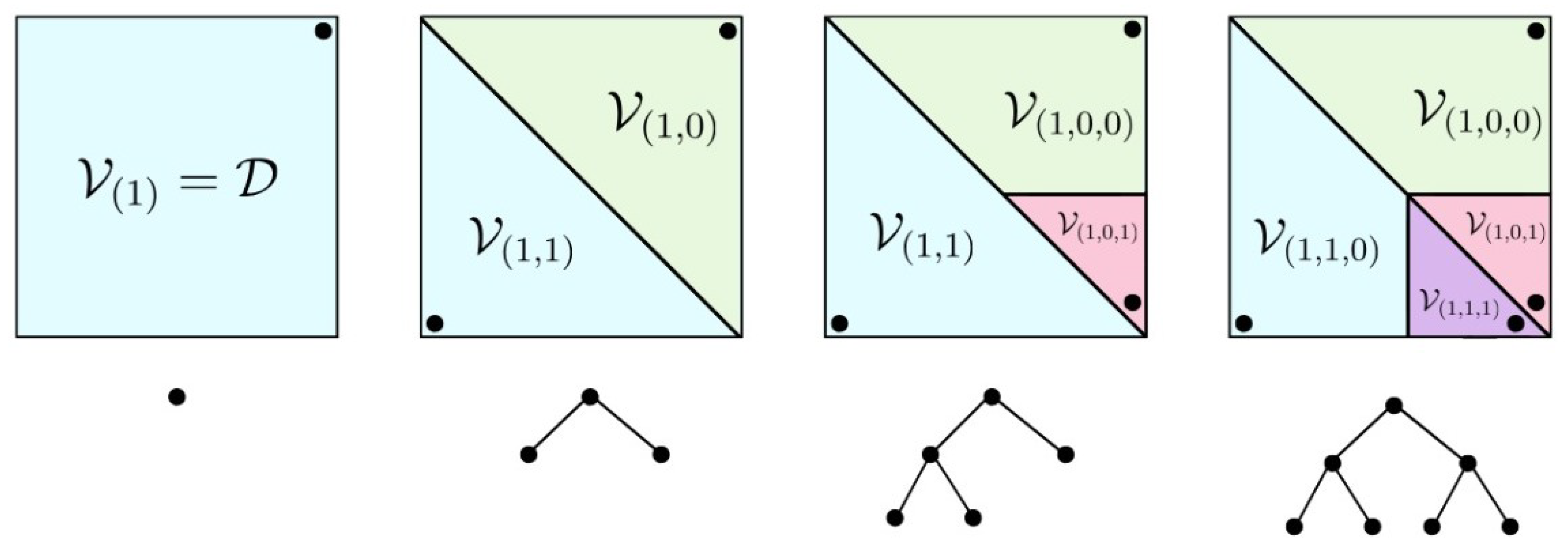
• The maximum depth $l_{max}$ of the resulting tree (briefly described in the next section), which limits the number of recursive partitions. As with any tree in ML, deeper trees lead to higher accuracies when training but, at the same time, they risk overfitting.

The previous discussion motivates the subject of this paper: our approach of an hp-greedy reduced basis requires an efficient search for an optimal choice of the hp-greedy hyperparameters. This is referred to as hyperparameter optimization (HPO) in the ML field. Here, we follow a Bayesian approach; more precisely, we adopt Sequential Model-Based Optimization (SMBO) through a Tree-Structured Parzen Estimator (TPE) [48], as implemented in the OPTUNA open source package [49].

The rest of the paper is organized as follows. In Section 2, we briefly review the hp-greedy reduced basis approach. In Section 3, we state the hyperparameter optimization problem and very briefly summarize some key elements of how we approach it using Bayesian optimization, SMBO, and TPE. We also include a benchmark comparison of BO and grid search for the Himmelblau function, which is commonly used in optimization tests. In Section 4, we present our results for the collision of two non-precessing aligned-spin black holes, the same physical setup that we used in our previous work [45]. We close in Section 5, presenting the conclusions of this work and potential future paths.

2. hp-Greedy Reduced Basis

The reduced basis-greedy approach finds a quasi-optimal—in a rigorous mathematical sense—low-dimensional approximation of a dataset with respect to the Kolmogorov n-width [50,51]. When applied to gravitational waves, the dataset consists of parameterized waveforms, for example, by the mass and spin of each object in the case of a compact binary coalescence. To further accelerate online evaluations and data analysis, a divide-and-conquer strategy can be pursued, which recursively partitions the parameter space and builds local reduced bases of lower dimensionality. We therefore proposed, in Ref. [45], a data-driven version of the hp-greedy approach [46] as a way of improving the construction of reduced bases within gravitational wave science.

As a summary, the hp-greedy approach generalizes the standard reduced-basis framework, allowing for the partitioning of the parameter space by combining reduced basis functions (p-refinement) with an adaptive grid (h-refinement). Each subspace can be assigned to a node in a binary tree structure. If a subspace is partitioned, it is associated with a node of the tree and, after partitioning it, each of the obtained subspaces is associated with a children node. In this way, the root of the tree represents the full parameter space. For more details, see Ref. [45].

The process builds a set of local reduced bases with several stopping criteria for partitioning the parameter domain: a maximum dimension $n_{max}$ for each local basis, a maximum depth $l_{max}$ of the tree, and an accuracy threshold ${ϵ}_{tol}$ as defined later on by Equation (5) (it is the usual definition in the reduced basis context). Until any of these stopping criteria are met, the domain gets partitioned, and reduced bases for the resulting subdomains are built. Figure 1 shows an example of a partition structure for a domain with $l_{max}=2$.

The hp-greedy approach is driven by the idea that, if the greedy error decreases slowly, leading to a large number of iterations, domain partitioning can help improve accuracy, which is similar in spirit to spectral elements in numerical solutions of partial differential equations [52]. The choice of partitioning is influenced by the rate of error reduction, which varies depending on the problem. Numerical experiments in our previous paper have demonstrated the effectiveness of the hp-greedy approach for gravitational waves, reducing basis dimensionality while maintaining accuracy (cf. Figure 12 of Ref. [45]).

The algorithm involves performing a binary domain-decomposition, and for traversing the resulting tree one can take advantage of its structure; we discuss this in Section 5. The hp-greedy approach is particularly useful for problems with physical discontinuities in the parameter space (cf. Section III of reference [45]).

An interesting finding of our experiments with hp-greedy is that the initial seed of the algorithm does affect the partitioning and subsequent reduced bases, and significantly impacts their accuracy. This differs from the standard global reduced basis approach, in which the seed choice is irrelevant (see, for example, Figure 1 of [47] and its corresponding discussion). Hence, the optimization of hyperparameters such as $l_{max}$ and the seed ${\widehat{\Lambda }}_0$ turns out to be crucial in the hp-greedy approach. This observation is the key motivation for this paper. The optimization task can be carried out through hyperparameter optimization in the ML sense.

3. Hyperparameter Optimization

An HPO problem can be stated as follows: given a cost function $f:X\to \mathbb{R}$ which returns the maximum validation error of a model trained with a combination of hyperparameters $\mathbf{x}\in X$, the goal is to find ${\mathbf{x}}^{*}$, such that

$${\mathbf{x}}^{*}=arg\underset{\mathbf{x}\in X}{min}f\left(\mathbf{x}\right).$$

In our context, we are interested in the optimal combination of hyperparameters from a domain X that gets the minimum representation error for a validation set. For a discussion of our results on test sets, see Section 4.3.

In the hp-greedy approach, each value of the tuple $\mathbf{x}$ represents a configuration of the two relevant hyperparameters for our scenario:

$$\mathbf{x}=(l_{max},{\widehat{\Lambda }}_0),$$

for fixed values of $n_{max}$. We decided to keep the latter fixed since the evaluation cost of both a surrogate based on reduced bases, and the computation of likelihoods using ROQ, is linear with the dimensionality of the basis, so we place it in a different hierarchy.

In practice, the cost function (which we have not defined yet) does not have a closed form expression, but is instead the result of training a model and evaluating the representation error of a validation set. This aspect usually makes the optimization problem computationally expensive.

Several HPO approaches have been and are being developed, with one of the driving motivations nowadays being deep neural networks. Two well-known HPO techniques are grid and random searches, although they are often inefficient in computational terms since the whole space is blindly explored. A more promising technique in this regard is Bayesian optimization [53,54], which was chosen for our problem. It attempts to minimize the number of evaluations of f to find ${\mathbf{x}}^{*}$ and falls within the category of Sequential Model-Based Optimization (SMBO) [48,55]. In this work, we rely on the Tree-Structured Parzen Estimator (TPE) [48] algorithm for Bayesian optimization. Besides being one of the simplest algorithms, it works well with discrete search spaces, scales linearly with the number of dimensions, and is optimized, as opposed to other methods such as Gaussian Processes (see [48] for more details). For the SMBO implementation, we used the Python package OPTUNA [49].

In Section 3.4, we present some results using Bayesian optimization alongside those from grid and random searches to quantify the advantages and computational savings of the former.

3.1. Bayesian Optimization

In essence, Bayesian optimization is an adaptive method that uses the information from previous evaluations of the cost function f to decide which value of $\mathbf{x}$ should be used next, with the goal of reducing the number of necessary evaluations of f to find a (in general, local) minimum (see Figure 2). To give a very brief list of some key elements behind this method, we begin with a description of SMBO.

3.2. Sequential Model-Based Optimization (SMBO)

The general idea is to approximate the cost function f with a substitute model $\mathcal{M}$. We start with a set of observations

$$D=\{({\mathbf{x}}^{\left(1\right)},y^{\left(1\right)}),\cdots ,({\mathbf{x}}^{\left(k\right)},y^{\left(k\right)})\},$$

(1)

with $y^{\left(j\right)}=f\left({\mathbf{x}}^{\left(j\right)}\right)$. Departing from this set, the substitute model $\mathcal{M}$ is adjusted. Next, using the predictions of the model, an acquisition function S is maximized. This function chooses the next set of hyperparameters ${\mathbf{x}}_i\in X$ to evaluate f, and the pair $({\mathbf{x}}_i,f\left({\mathbf{x}}_i\right))$ is added to the observation set D. After that, $\mathcal{M}$ is adjusted again, and the process is repeated for a fixed number of iterations. This procedure is captured by the pseudocode given in Algoritm 1.

Algorithm 1: SMBO

input: $f,X,S,\mathcal{M}$    $f:\mathrm{Objective}\mathrm{function}$,    $X:\mathrm{Search}\mathrm{space}$,   $\mathcal{M}:\mathrm{Model},$   $S:\mathrm{Acquisition}\mathrm{function}.$ 1: $D=$ InitialSample$(f,X)$   2: for $i=1,2,...$ do 3:    $\mathcal{M}=$ AdjustModel$\left(D\right)$ 4:    ${\mathbf{x}}_i=arg{max}_{\mathbf{x}\in X}\mathcal{S}(\mathbf{x},\mathcal{M})$. 5:    $y_i=f\left({\mathbf{x}}_i\right)$ 6:    $D=D\cup \left\{({\mathbf{x}}_i,y_i)\right\}$ 7: end for

Using Bayes’ theorem, if $P\left(y\right|\mathbf{x})$ is the posterior probability, $P\left(y\right)$ the prior, and $P\left(\mathbf{x}\right|y)$ the likelihood, then

$$P\left(y\right|\mathbf{x})=\frac{P\left(\mathbf{x}\right|y\left)P\right(y)}{P\left(\mathbf{x}\right)}.$$

In a Bayesian approach to SMBO, $P\left(y\right|\mathbf{x})$ is the prediction of the model, with y being an evaluation of $f\left(\mathbf{x}\right)$.

We mentioned that, for selecting the points to evaluate, an acquisition function S is maximized. Several proposals exist for choosing the acquisition function. In this work, we use the Expected Improvement (EI) [57] criterion: if $y^{*}$ is a reference value, then EI with respect to $y^{*}$ is defined as

$$E{I}_{y^{*}}\left(\mathbf{x}\right):={\int }_{-\infty }^{\infty }max(y^{*}-y,0)P\left(y\right|\mathbf{x})dy.$$

(2)

3.3. Tree-Structured Parzen Estimator

The Tree-Structured Parzen Estimator (TPE) [48] is a strategy to model $P\left(x_i\right|y)$ for each $x_i\in X_i$ (that is, each $x_i$ represents a different hyperparameter) from two distributions built using the observations D (1):

$$P\left(x_i\right|y)=\left\{\begin{array}{cc}\ell \left(x_i\right)\hfill & \mathrm{if}y<y^{*}\hfill \\ g\left(x_i\right)\hfill & \mathrm{if}y\ge y^{*}.\hfill \end{array}\right.$$

(3)

Here, the densities $\{\ell \left(x_i\right),g\left(x_i\right)\}$ are built from two sets $\{D_{\ell },D_g\}\subset D$, such that $D_{\ell }$ has all the observations with $y<y^{*}$, $D_g$ the remaining ones, and $D=D_{\ell }\cup D_g$.

The reference value $y^{*}$ is a quantile $\gamma \in (0,1)$ of the observed values, so that the prior is

$$P(y<y^{*})=\gamma .$$

This means that $y^{*}$ is a certain value between the best y and worst y found at some iteration (e.g., if $\gamma$ is equal to $0.5$, then $y^{*}$ is equal to the median of the observed values of y).

Building $\ell \left(x_i\right)$ and $g\left(x_i\right)$ implies adjusting the model (line 3 in Algorithm 1), and then using (3) in the definition of the expected improvement (2). In order to maximize the expected improvement (step 4 in Algorithm 1), one has to choose a value of $x_i$ that maximizes the ratio $\ell \left(x_i\right)/g\left(x_i\right)$ (see [48] for more details):

$$x_i^{*}=arg\underset{x_i}{max}\left(\ell \left(x_i\right)/g\left(x_i\right)\right).$$

(4)

In summary, the TPE algorithm constructs two probability density functions:

• $\ell \left(x_i\right)$ using “good” observations ($y<y^{*}$); and
• $g\left(x_i\right)$ using “bad” observations ($y\ge y^{*}$).

These functions are updated every time the objective function is evaluated (at every iteration of the algorithm), and the new $x_i$ is chosen by maximizing $\ell \left(x_i\right)/g\left(x_i\right)$, implying that the new $x_i$ is much more likely to represent a good observation rather than a bad one.

All density functions are constructed using Parzen estimators [58]. For each point $x_i$, a truncated normal distribution centered at that point is added. A way to think of a Parzen window is to visualize it as a smoothed histogram. The choice of truncated normal distributions for the kernel function is presented in the original TPE paper [48]. For more details about the implementation of the Parzen estimator in OPTUNA, see Ref. [59].

3.4. A Comparison between HPO, Grid, and Random Searches

We compare grid and random searches against Bayesian optimization. To this end, we consider the Himmelblau function, which is a widely used benchmark in optimization and ML, as the objective function to be minimized. This function is shown in Figure 3 and is defined as follows:

$$f(x,y)={(x^2+y-11)}^2+{(x+y^2-7)}^2.$$

Here, we simplistically assume that the Himmelblau function represents the accuracy of an ML model, where each input of the function represents a set of hyperparameters of the algorithm and the outcome is the resulting accuracy. The objective is to obtain a set of values that minimizes the function. We show results for these three methods: grid and random searches, and Bayesian optimization. For each case, 100 different evaluations were used. Then, we assess which one performed better.

Figure 4 shows the search patterns resulting from each approach. After 100 trials, Bayesian optimization found the lowest value among the three methods (recall that the four local minima are at $f=0$), with $f=0.09$, while random search found $f=1.71$ and grid search found $f=3.68$. As can be seen from Figure 4, Bayesian optimization has the advantage of exploring the search space adaptively, leading to faster convergence when compared to grid or random searches. This is so because neither grid nor random search keeps evidence from older trials, which makes them less effective than a Bayesian approach.

This example showcases the key features of Bayesian optimization, which are its efficiency (i.e., number of trials to reach a minimum), adaptive search, and relatively low computational effort.

4. Hyper-Optimized hp-Greedy Reduced Bases for Gravitational Waves

In this section, we apply the hp-greedy approach to build accurate and low-dimensional representations of gravitational waves, optimizing the choice of hyperparameters with a Bayesian approach, as described in the previous section.

In our numerical experiments, we found that the cost function to optimize is considerably more complex than the Himmelblau function of the previous section, with lots of structure and many sharp local minima.

4.1. Physical Setup

The waveforms used to train hp-greedy and perform HPO were obtained from NRHybSur3dq8 [60]. This is a surrogate model for hybridized non-precessing numerical relativity and post-Newtonian waveforms within the parameter range of mass ratios $1\le q\le 8$, and dimensionless spins $-0.8\le {\chi }_{1z},{\chi }_{2z}\le 0.8$. In this work, we focus on the dominant angular mode $l=m=2$ of the waveforms, which we sampled in the late inspiral and merger phases, with $t\in [-2750,100]M$, and a time step of $\Delta t=0.1M$. Additionally, we normalized the waveforms with respect to the ${\ell }_2$ norm to emphasize structural characteristics rather than size or amplitude.

In this paper, we focus on two distinct cases:

• 1D Case: This scenario involves no spin, where the sole free parameter is the mass ratio, $q:=m_1/m_2$.
• 2D Case: Two spins aligned in the same direction and with equal magnitudes, ${\chi }_{1z}={\chi }_{2z}$, are added to the 1D scenario.

In both cases, we generated multiple training sets of different sizes, as shown in SubSection 4.3. As an error metric for the reduced basis representation ${\tilde{h}}_{\lambda }\left(t\right)$ of a waveform $h_{\lambda }\left(t\right)$ labeled by the parameter $\lambda$, we use the usual one in a greedy context, namely the maximum in the parameter space of the ${\ell }_2$ norm,

$$ϵ:=\underset{\lambda }{max}{\parallel h_{\lambda }(·)-{\tilde{h}}_{\lambda }(·)\parallel }^2,$$

(5)

where ${\tilde{h}}_{\lambda }\left(t\right):=\mathcal{P}{h}_{\lambda }\left(t\right)$ is the orthogonal projection of $h_{\lambda }\left(t\right)$ onto the span of the (reduced) basis. For the quadratures involved in the computation of the 2-norm, we used Riemann’s rule.

4.2. Optimization Methods Compared

In Section 3.4, we compared the TPE algorithm with random and grid searches. Here, we benchmark these methods in the context of gravitational waves using a small dataset in the 1D case. We used 400 waveforms for training and 800 for validation, all equally spaced in the 1D parameter domain ($1<q<8$).

The hyperparameters being optimized were $l_{max}$, with

$$0\le l_{max}\le 7,$$

and the seed ${\widehat{\Lambda }}_0$, with 400 different values. Along with 8 possible $l_{max}$ values, this leads to a search space of 3200 different configurations.

The value of $l_{max}$ is manually chosen, here and in the other experiments of this paper, so that the (a posteriori found) optimized values turn out to be below such a maximum.

Since we have a discrete search space, we can go through all the different configurations with one grid search. We divide the comparison into two parts:

• On the convergence speed of TPE compared to random search, and how consistent it is through multiple runs.
• On the time difference between grid search and one run of TPE.

In Figure 5, we show the results of running 150 optimizations for TPE and random search; each point is the median of the best validation error found for the 150 optimizations at a given time, and the area of color represents the Q1 and Q3 quartiles ($0.25$ and $0.75$, respectively).

The black dashed lines show the best error found with grid search. We can see that the TPE curve is always below the random one, and that the colored area reduces drastically at around 70 s of optimization for TPE, which consistently finds good results after this point.

The optimum value found by grid search was a validation error of $1.23\times {10}^{-7}$. This value was found on $19\%$ of the TPE runs, while the other $81\%$ found the second best value: $1.59\times {10}^{-7}$. On the other hand, none of the random search runs were able to find the optimum value, and only $10\%$ found the second best value of $1.59\times {10}^{-7}$. These results show that TPE can find better results than random searches, in less time, and more consistently.

Grid search took $9.8$ hours to complete for the 3200 configurations of this experiment; meanwhile, the 50 iterations needed by TPE took about 5 min. This is a difference of two orders of magnitude, a factor of $117\times$ times in speedup. In a more realistic optimization task, for example, using 5000 waveforms for training and $10,000$ for validation and a total of $50,000$ hyperparameter configurations, 100 iterations of TPE would take around 16 h. Using these values, we can estimate that a grid search would take, in contrast, around 8000 hours, or 11 months to complete. Thus, grid search is not a viable method for finding an optimal configuration in any realistic scenario.

All of these runs were performed in the Serafín cluster from CCAD-UNC 3, where each node consists of 2 AMD EPYC 7532 of 200W with 32 cores of Zen2 microarchitecture, with 128 GiB of RAM DDR4-3200.

4.3. Optimized hp-Greedy Reduced Bases versus Global Ones

Now, we present our results for Bayesian HPO and the hp-greedy approach for the gravitational waveforms setup described in Section 4.1 for the hyperparameters

$$\{{\widehat{\Lambda }}_0,l_{max}\},$$

with fixed maximum dimensionalities $n_{max}$ of each reduced basis and $l_{max}=10$ and 20 for the 1D and 2D cases, respectively. The accuracy threshold in all cases is chosen to be $ϵ={10}^{-7}$, which is the systematic error of the underlying model, NRHybSur3dq8 [60].

The learning curves of Figure 6 show the validation error achieved for each optimized hp-greedy reduced basis; the intent of these plots is to determine when a training set is dense enough. For example, in the 1D case, around 2000 training samples are enough, while, in the 2D case, this number grows to ∼15,000, which is smaller than $2000\times 2000$ and shows that there is increased redundancy in the waveforms as the dimensionality grows.

We are interested in the smallest $n_{max}$ for each case, since this implies the fastest online waveform evaluation and data analysis in general; these are $n_{max}=3$ and 10 for the 1D and 2D cases, respectively. When compared to global bases, the hyperparameter-optimized hp-greedy bases are 4–5 times smaller, which should translate into a factor of (4–5)× speedup both in waveform evaluation but, most importantly, in parameter estimation. The benefit of using a reduced hp-greedy basis instead of a global one can be seen in Figure 7.

5. Discussion

In this paper, we continued our work on local, unstructured reduced bases for gravitational waves using hp-greedy refinement, with the aim of accelerating both waveform predictions and inference (especially parameter estimation). In reference [45], we found that there are new hyperparameters to be optimized, which do not appear in global reduced bases. As usual in the ML context, parameters are learned from training, while hyperparameters remain fixed during each training stage.

The resulting structure of hp-greedy reduced bases is one of a binary tree. In our simulations, though limited in size, we have empirically found that the trees of hp-greedy refinement end up being nearly balanced. When a representation is needed for a given parameter, the corresponding local basis can be searched for in the representation tree in an efficient way, avoiding the computational cost of a direct/naive search. To do so, two sequential steps are needed: (i) find the subspace containing the local reduced basis, and (ii) use that basis for the representation. The search utilizes $\lambda$ as input and the hp-greedy tree structure to traverse the tree from the root to a leaf node, which contains the queried value of $\lambda$ in its subspace (see Equation (4.13) of [46] for more details). The advantage of this approach is the low computational cost to find the required subspace; for example, if there are n subspaces and the tree is balanced, the computational cost is of order $\mathcal{O}$(log n).

There are several stopping criteria for subdividing the parameter domain and avoiding overfitting. In this work, we have taken them to be $n_{max}$ (maximum dimensionality of each local reduced basis), $l_{max}$ (maximum depth of the tree), and the error ${ϵ}_{tol}$; in practice, the latter should not be smaller than the underlying systematical error of the data.

Our results show that using a Bayesian approach is a promising path to HPO. Nonetheless, there are other alternatives, such as evolutionary programming or genetic algorithms, which were left out of the scope of this paper and could be analyzed in future work if need be. Another approach, suggested by an anonymous referee to whom we are extremely grateful, would be to perform (potentially parallelized) grid searches on $l_{max}$ (since it takes discrete values) and a gradient descent with, for example, BFGS (a quasi-Newtonian method). There are many options which can be studied within the context of the rich structure of the cost function of the HPO problem of the hp-greedy approach; here, we focused on one which worked well and efficiently for our purposes.

In conjunction with the computations outlined in the paper, we have made the corresponding codes available on GitHub. These repositories contain the codebase for the Bayesian optimization [61] and hp-greedy models [62] used in this paper.

While preparing this manuscript, a different approach [63] to obtain multiple local reduced bases of lower dimensionality, by manually partitioning the parameter domain and multi-banding, appeared in the literature. Since the partitioning is manual, it seems that there are no hyperparameters involved and, therefore, no HPO needed.

References

- Tiglio, M.; Villanueva, A. Reduced order and surrogate models for gravitational waves. Living Rev. Relativ. 2022, 25, 2. [Google Scholar] [CrossRef]
- Mandic, V.; Thrane, E.; Giampanis, S.; Regimbau, T. Parameter estimation in searches for the stochastic gravitational-wave background. Phys. Rev. Lett. 2012, 109, 171102. [Google Scholar] [CrossRef]
- Isi, M.; Chatziioannou, K.; Farr, W.M. Hierarchical test of general relativity with gravitational waves. Phys. Rev. Lett. 2019, 123, 121101. [Google Scholar] [CrossRef] [PubMed]
- Lange, J.; O’Shaughnessy, R.; Rizzo, M. Rapid and accurate parameter inference for coalescing, precessing compact binaries. arXiv 2018, arXiv:1805.10457. [Google Scholar]
- Lynch, R.; Vitale, S.; Essick, R.; Katsavounidis, E.; Robinet, F. Information-theoretic approach to the gravitational-wave burst detection problem. Phys. Rev. D 2017, 95, 104046. [Google Scholar] [CrossRef]
- Mandel, I.; Berry, C.P.; Ohme, F.; Fairhurst, S.; Farr, W.M. Parameter estimation on compact binary coalescences with abruptly terminating gravitational waveforms. Class. Quantum Gravity 2014, 31, 155005. [Google Scholar] [CrossRef]
- Mandel, I.; Farr, W.M.; Gair, J.R. Extracting distribution parameters from multiple uncertain observations with selection biases. Mon. Not. R. Astron. Soc. 2019, 486, 1086–1093. [Google Scholar] [CrossRef]
- Usman, S.A.; Mills, J.C.; Fairhurst, S. Constraining the inclinations of binary mergers from gravitational-wave observations. Astrophys. J. 2019, 877, 82. [Google Scholar] [CrossRef]
- Van Der Sluys, M.; Mandel, I.; Raymond, V.; Kalogera, V.; Röver, C.; Christensen, N. Parameter estimation for signals from compact binary inspirals injected into LIGO data. Class. Quantum Gravity 2009, 26, 204010. [Google Scholar] [CrossRef]
- Fishbach, M.; Essick, R.; Holz, D.E. Does Matter Matter? Using the mass distribution to distinguish neutron stars and black holes. Astrophys. J. Lett. 2020, 899, L8. [Google Scholar] [CrossRef]
- Cornish, N.J. Rapid and robust parameter inference for binary mergers. Phys. Rev. D 2021, 103, 104057. [Google Scholar] [CrossRef]
- Berry, C.P.; Mandel, I.; Middleton, H.; Singer, L.P.; Urban, A.L.; Vecchio, A.; Vitale, S.; Cannon, K.; Farr, B.; Farr, W.M.; et al. Parameter estimation for binary neutron-star coalescences with realistic noise during the Advanced LIGO era. Astrophys. J. 2015, 804, 114. [Google Scholar] [CrossRef]
- Biscoveanu, S.; Haster, C.J.; Vitale, S.; Davies, J. Quantifying the effect of power spectral density uncertainty on gravitational-wave parameter estimation for compact binary sources. Phys. Rev. D 2020, 102, 023008. [Google Scholar] [CrossRef]
- Bizouard, M.A.; Maturana-Russel, P.; Torres-Forné, A.; Obergaulinger, M.; Cerdá-Durán, P.; Christensen, N.; Font, J.A.; Meyer, R. Inference of protoneutron star properties from gravitational-wave data in core-collapse supernovae. Phys. Rev. D 2021, 103, 063006. [Google Scholar] [CrossRef]
- Banagiri, S.; Coughlin, M.W.; Clark, J.; Lasky, P.D.; Bizouard, M.A.; Talbot, C.; Thrane, E.; Mandic, V. Constraining the gravitational-wave afterglow from a binary neutron star coalescence. Mon. Not. R. Astron. Soc. 2020, 492, 4945–4951. [Google Scholar] [CrossRef]
- Coughlin, M.W.; Dietrich, T.; Margalit, B.; Metzger, B.D. Multimessenger Bayesian parameter inference of a binary neutron star merger. Mon. Not. R. Astron. Soc. Lett. 2019, 489, L91–L96. [Google Scholar] [CrossRef]
- Wysocki, D.; Lange, J.; O’Shaughnessy, R. Reconstructing phenomenological distributions of compact binaries via gravitational wave observations. Phys. Rev. D 2019, 100, 043012. [Google Scholar] [CrossRef]
- Christensen, N.; Meyer, R. Parameter estimation with gravitational waves. Rev. Mod. Phys. 2022, 94, 025001. [Google Scholar] [CrossRef]
- Jaranowski, P.; Królak, A. Gravitational-wave data analysis. Formalism and sample applications: The Gaussian case. Living Rev. Relativ. 2012, 15, 1–47. [Google Scholar] [CrossRef]
- Smith, R.; Borhanian, S.; Sathyaprakash, B.; Vivanco, F.H.; Field, S.E.; Lasky, P.; Mandel, I.; Morisaki, S.; Ottaway, D.; Slagmolen, B.J.; et al. Bayesian inference for gravitational waves from binary neutron star mergers in third generation observatories. Phys. Rev. Lett. 2021, 127, 081102. [Google Scholar] [CrossRef]
- Breschi, M.; Gamba, R.; Bernuzzi, S. Bayesian inference of multimessenger astrophysical data: Methods and applications to gravitational waves. Phys. Rev. D 2021, 104, 042001. [Google Scholar] [CrossRef]
- Chua, A.J.; Vallisneri, M. Learning Bayesian posteriors with neural networks for gravitational-wave inference. Phys. Rev. Lett. 2020, 124, 041102. [Google Scholar] [CrossRef] [PubMed]
- Meyer, R.; Edwards, M.C.; Maturana-Russel, P.; Christensen, N. Computational techniques for parameter estimation of gravitational wave signals. Wiley Interdiscip. Rev. Comput. Stat. 2022, 14, e1532. [Google Scholar] [CrossRef]
- Edwards, M.C.; Meyer, R.; Christensen, N. Bayesian parameter estimation of core collapse supernovae using gravitational wave simulations. Inverse Probl. 2014, 30, 114008. [Google Scholar] [CrossRef][Green Version]
- Dupuis, R.J.; Woan, G. Bayesian estimation of pulsar parameters from gravitational wave data. Phys. Rev. D 2005, 72, 102002. [Google Scholar] [CrossRef]
- Talbot, C.; Smith, R.; Thrane, E.; Poole, G.B. Parallelized inference for gravitational-wave astronomy. Phys. Rev. D 2019, 100, 043030. [Google Scholar] [CrossRef]
- Veitch, J.; Raymond, V.; Farr, B.; Farr, W.; Graff, P.; Vitale, S.; Aylott, B.; Blackburn, K.; Christensen, N.; Coughlin, M.; et al. Parameter estimation for compact binaries with ground-based gravitational-wave observations using the LALInference software library. Phys. Rev. D 2015, 91, 042003. [Google Scholar] [CrossRef]
- Biwer, C.M.; Capano, C.D.; De, S.; Cabero, M.; Brown, D.A.; Nitz, A.H.; Raymond, V. PyCBC Inference: A Python-based parameter estimation toolkit for compact binary coalescence signals. Publ. Astron. Soc. Pac. 2019, 131, 024503. [Google Scholar] [CrossRef]
- Ashton, G.; Hübner, M.; Lasky, P.D.; Talbot, C.; Ackley, K.; Biscoveanu, S.; Chu, Q.; Divakarla, A.; Easter, P.J.; Goncharov, B.; et al. BILBY: A user-friendly Bayesian inference library for gravitational-wave astronomy. Astrophys. J. Suppl. Ser. 2019, 241, 27. [Google Scholar] [CrossRef]
- Romero-Shaw, I.M.; Talbot, C.; Biscoveanu, S.; D’emilio, V.; Ashton, G.; Berry, C.; Coughlin, S.; Galaudage, S.; Hoy, C.; Hübner, M.; et al. Bayesian inference for compact binary coalescences with bilby: Validation and application to the first LIGO–Virgo gravitational-wave transient catalogue. Mon. Not. R. Astron. Soc. 2020, 499, 3295–3319. [Google Scholar] [CrossRef]
- Smith, R.J.; Ashton, G.; Vajpeyi, A.; Talbot, C. Massively parallel Bayesian inference for transient gravitational-wave astronomy. Mon. Not. R. Astron. Soc. 2020, 498, 4492–4502. [Google Scholar] [CrossRef]
- Wofford, J.; Yelikar, A.; Gallagher, H.; Champion, E.; Wysocki, D.; Delfavero, V.; Lange, J.; Rose, C.; Valsan, V.; Morisaki, S.; et al. Expanding RIFT: Improving performance for GW parameter inference. arXiv 2022, arXiv:2210.07912. [Google Scholar]
- Dax, M.; Green, S.R.; Gair, J.; Macke, J.H.; Buonanno, A.; Schölkopf, B. Real-time gravitational wave science with neural posterior estimation. Phys. Rev. Lett. 2021, 127, 241103. [Google Scholar] [CrossRef]
- Antil, H.; Field, S.E.; Herrmann, F.; Nochetto, R.H.; Tiglio, M. Two-Step Greedy Algorithm for Reduced Order Quadratures. J. Sci. Comput. 2013, 57, 604–637. [Google Scholar] [CrossRef]
- Canizares, P.; Field, S.E.; Gair, J.R.; Tiglio, M. Gravitational wave parameter estimation with compressed likelihood evaluations. Phys. Rev. D 2013, D87, 124005. [Google Scholar] [CrossRef]
- Canizares, P.; Field, S.E.; Gair, J.; Raymond, V.; Smith, R.; Tiglio, M. Accelerated gravitational wave parameter estimation with reduced order modeling. Phys. Rev. Lett. 2015, 114, 071104. [Google Scholar] [CrossRef]
- Barrault, M.; Maday, Y.; Nguyen, N.C.; Patera, A.T. An ‘empirical interpolation’method: Application to efficient reduced-basis discretization of partial differential equations. Comptes Rendus Math. 2004, 339, 667–672. [Google Scholar] [CrossRef]
- Gabbard, H.; Messenger, C.; Heng, I.S.; Tonolini, F.; Murray-Smith, R. Bayesian parameter estimation using conditional variational autoencoders for gravitational-wave astronomy. arXiv 2019, arXiv:1909.06296. [Google Scholar] [CrossRef]
- Green, S.; Gair, J. Complete parameter inference for GW150914 using deep learning. arXiv 2020, arXiv:2008.03312. [Google Scholar] [CrossRef]
- Green, S.R.; Simpson, C.; Gair, J. Gravitational-wave parameter estimation with autoregressive neural network flows. Phys. Rev. D 2020, 102, 104057. [Google Scholar] [CrossRef]
- George, D.; Huerta, E. Deep learning for real-time gravitational wave detection and parameter estimation with LIGO data. arXiv 2017, arXiv:1711.07966. [Google Scholar] [CrossRef]
- Álvares, J.D.; Font, J.A.; Freitas, F.F.; Freitas, O.G.; Morais, A.P.; Nunes, S.; Onofre, A.; Torres-Forné, A. Exploring gravitational-wave detection and parameter inference using deep learning methods. Class. Quantum Gravity 2021, 38, 155010. [Google Scholar] [CrossRef]
- Shen, H.; Huerta, E.; O’Shea, E.; Kumar, P.; Zhao, Z. Statistically-informed deep learning for gravitational wave parameter estimation. Mach. Learn. Sci. Technol. 2021, 3, 015007. [Google Scholar] [CrossRef]
- Morisaki, S.; Raymond, V. Rapid Parameter Estimation of Gravitational Waves from Binary Neutron Star Coalescence using Focused Reduced Order Quadrature. Phys. Rev. D 2020, 102, 104020. [Google Scholar] [CrossRef]
- Cerino, F.; Diaz-Pace, J.A.; Tiglio, M. An automated parameter domain decomposition approach for gravitational wave surrogates using hp-greedy refinement. Class. Quant. Grav. 2023, 40, 205003. [Google Scholar] [CrossRef]
- Eftang, J.L. Reduced Basis Methods for Parametrized Partial Differential Equations; Norwegian University of Science and Technology: Trondheim, Norway, 2011. [Google Scholar]
- Caudill, S.; Field, S.E.; Galley, C.R.; Herrmann, F.; Tiglio, M. Reduced Basis representations of multi-mode black hole ringdown gravitational waves. Class. Quant. Grav. 2012, 29, 095016. [Google Scholar] [CrossRef][Green Version]
- Bergstra, J.; Bardenet, R.; Bengio, Y.; Kégl, B. Algorithms for Hyper-Parameter Optimization. In Advances in Neural Information Processing Systems; Shawe-Taylor, J., Zemel, R., Bartlett, P., Pereira, F., Weinberger, K., Eds.; Curran Associates, Inc.: Red Hook, NY, USA, 2011; Volume 24. [Google Scholar]
- Akiba, T.; Sano, S.; Yanase, T.; Ohta, T.; Koyama, M. Optuna: A Next-generation Hyperparameter Optimization Framework. In Proceedings of the 25rd ACM SIGKDD International Conference on Knowledge Discovery and Data Mining, Anchorage, AK, USA, 4–8 August 2019. [Google Scholar]
- Binev, P.; Cohen, A.; Dahmen, W.; DeVore, R.A.; Petrova, G.; Wojtaszczyk, P. Convergence Rates for Greedy Algorithms in Reduced Basis Methods. SIAM J. Math. Anal. 2011, 43, 1457–1472. [Google Scholar] [CrossRef]
- DeVore, R.; Petrova, G.; Wojtaszczyk, P. Greedy Algorithms for Reduced Bases in Banach Spaces. Constr. Approx. 2013, 37, 455–466. [Google Scholar] [CrossRef]
- Karniadakis, G.; Sherwin, S.J. Spectral/hp Element Methods for Computational Fluid Dynamics, 2nd ed.; Oxford University Press: Oxford, UK, 2005. [Google Scholar] [CrossRef]
- Shahriari, B.; Swersky, K.; Wang, Z.; Adams, R.P.; de Freitas, N. Taking the Human Out of the Loop: A Review of Bayesian Optimization. Proc. IEEE 2016, 104, 148–175. [Google Scholar] [CrossRef]
- Brochu, E.; Cora, V.M.; de Freitas, N. A Tutorial on Bayesian Optimization of Expensive Cost Functions, with Application to Active User Modeling and Hierarchical Reinforcement Learning. arXiv 2010, arXiv:1012.2599. [Google Scholar] [CrossRef]
- Dewancker, I.; McCourt, M.; Clark, S. Bayesian Optimization Primer; SigOpt: San Francisco, CA, USA, 2015. [Google Scholar]
- Feurer, M.; Hutter, F. Hyperparameter Optimization. In Automated Machine Learning: Methods, Systems, Challenges; Hutter, F., Kotthoff, L., Vanschoren, J., Eds.; Springer International Publishing: Cham, Switzerland, 2019; pp. 3–33. [Google Scholar] [CrossRef]
- Jones, D. A Taxonomy of Global Optimization Methods Based on Response Surfaces. J. Glob. Optim. 2001, 21, 345–383. [Google Scholar] [CrossRef]
- Parzen, E. On Estimation of a Probability Density Function and Mode. Ann. Math. Stat. 1962, 33, 1065–1076. [Google Scholar] [CrossRef]
- Ozaki, Y.; Tanigaki, Y.; Watanabe, S.; Nomura, M.; Onishi, M. Multiobjective Tree-Structured Parzen Estimator. J. Artif. Int. Res. 2022, 73, 1209–1250. [Google Scholar] [CrossRef]
- Varma, V.; Field, S.E.; Scheel, M.A.; Blackman, J.; Kidder, L.E.; Pfeiffer, H.P. Surrogate model of hybridized numerical relativity binary black hole waveforms. Phys. Rev. D 2019, 99, 064045. [Google Scholar] [CrossRef]
- Villegas, A. hp-Greedy Bayesian Optimization. 2023. Available online: https://github.com/atuel96/hp-greedy-bayesian-optimization (accessed on 23 October 2023).
- Cerino, F. Scikit-ReducedModel. 2022. Available online: https://github.com/francocerino/scikit-reducedmodel (accessed on 12 October 2023).
- Morisaki, S.; Smith, R.; Tsukada, L.; Sachdev, S.; Stevenson, S.; Talbot, C.; Zimmerman, A. Rapid localization and inference on compact binary coalescences with the Advanced LIGO-Virgo-KAGRA gravitational-wave detector network. arXiv 2023, arXiv:2307.13380. [Google Scholar]
Disclaimer/Publisher’s Note: The statements, opinions and data contained in all publications are solely those of the individual author(s) and contributor(s) and not of MDPI and/or the editor(s). MDPI and/or the editor(s) disclaim responsibility for any injury to people or property resulting from any ideas, methods, instructions or products referred to in the content. |
© 2023 by the authors. Licensee MDPI, Basel, Switzerland. This article is an open access article distributed under the terms and conditions of the Creative Commons Attribution (CC BY) license (https://creativecommons.org/licenses/by/4.0/).
Share and Cite
Cerino, F.; Diaz-Pace, J.A.; Tassone, E.A.; Tiglio, M.; Villegas, A. Hyperparameter Optimization of an hp-Greedy Reduced Basis for Gravitational Wave Surrogates. Universe 2024, 10, 6. https://doi.org/10.3390/universe10010006
Cerino F, Diaz-Pace JA, Tassone EA, Tiglio M, Villegas A. Hyperparameter Optimization of an hp-Greedy Reduced Basis for Gravitational Wave Surrogates. Universe. 2024; 10(1):6. https://doi.org/10.3390/universe10010006
Chicago/Turabian StyleCerino, Franco, J. Andrés Diaz-Pace, Emmanuel A. Tassone, Manuel Tiglio, and Atuel Villegas. 2024. "Hyperparameter Optimization of an hp-Greedy Reduced Basis for Gravitational Wave Surrogates" Universe 10, no. 1: 6. https://doi.org/10.3390/universe10010006
APA StyleCerino, F., Diaz-Pace, J. A., Tassone, E. A., Tiglio, M., & Villegas, A. (2024). Hyperparameter Optimization of an hp-Greedy Reduced Basis for Gravitational Wave Surrogates. Universe, 10(1), 6. https://doi.org/10.3390/universe10010006