Abstract
In this paper, we explore the interior dynamics of neutral and charged black holes in gravity. We transform gravity from the Jordan frame into the Einstein frame and simulate scalar collapses in flat, Schwarzschild, and Reissner-Nordström geometries. In simulating scalar collapses in Schwarzschild and Reissner-Nordström geometries, Kruskal and Kruskal-like coordinates are used, respectively, with the presence of and a physical scalar field being taken into account. The dynamics in the vicinities of the central singularity of a Schwarzschild black hole and of the inner horizon of a Reissner-Nordström black hole is examined. Approximate analytic solutions for different types of collapses are partially obtained. The scalar degree of freedom ϕ, transformed from , plays a similar role as a physical scalar field in general relativity. Regarding the physical scalar field in case, when is negative (positive), the physical scalar field is suppressed (magnified) by ϕ, where t is the coordinate time. For dark energy gravity, inside black holes, gravity can easily push to 1. Consequently, the Ricci scalar R becomes singular, and the numerical simulation breaks down. This singularity problem can be avoided by adding an term to the original function, in which case an infinite Ricci scalar is pushed to regions where is also infinite. On the other hand, in collapse for this combined model, a black hole, including a central singularity, can be formed. Moreover, under certain initial conditions, and R can be pushed to infinity as the central singularity is approached. Therefore, the classical singularity problem, which is present in general relativity, remains in collapse for this combined model.
1. Introduction
The internal structure of black holes and spacetime singularities are key topics in gravitation and cosmology [1,2,3,4,5], and are great platforms to explore the connection between classical and quantum physics. It is widely believed that rotating black holes exist in reality. According to Price’s theorem, for a collapsing star, the gravitational radiation carries away all the initial features of the star’s gravitational field, except the mass, charge, and angular momentum parameters [6]. As a further step, it is natural to ask what the final state of the internal collapses might be.
Ever since the foundation of general relativity, people have been trying to go beyond it. This endeavor arises from unifying gravitation and quantum mechanics, and addressing some cosmological problems, including the singularity problem in the early Universe and the dark energy problem in the late Universe. Various modified gravity theories have been explored, including scalar-tensor theory, high-dimensional theory, and gravity, etc. For a review of modified gravity theories, see Reference [7]. For reviews of theory, see References [8,9,10,11].
Static and spherically symmetric black hole solutions in gravity were explored in Reference [12]. Charged Born-Infeld black holes for theories were studied in Reference [13]. Instabilities and (anti)-evaporation of Schwarzschild-de Sitter and Reissner-Nordström black holes in modified gravity were discussed in References [14,15,16].
Gravitational collapses in some modified gravity theories have been studied numerically. Spherical collapse of a neutral scalar field in a given spherical, charged black hole in Brans-Dicke theory was investigated in Reference [17]. Spherical collapses of a charged scalar field in dilaton gravity and gravity were explored in References [18] and [19], respectively. Spherical scalar collapse in gravity was simulated in Reference [20]. Asymptotic analysis was implemented in the vicinity of the singularity of a formed black hole.
1.1. Mass Inflation
In the vicinity of the central singularity inside a Schwarzschild black hole, the tidal force diverges, and maximal globally hyperbolic region defined by initial data is inextendible. However, inside charged (Reissner-Nordström) and rotating (Kerr) black holes, the central singularity is timelike. The globally hyperbolic region is up to the Cauchy horizon, and the spacetime is extendible beyond this horizon to a larger manifold. The Reissner-Nordström inner (Cauchy) horizon is a surface of infinite blueshift, which in turn may cause the inner horizon unstable [21]. Furthermore, the strong cosmic censorship conjecture was proposed, which states that for generic asymptotically flat initial data, the maximal Cauchy development is future inextendible. For mathematical explorations of the internal structures of charge black holes, see References [22,23]. For reviews on the Cauchy problem in general relativity and strong cosmic censorship, see References [24,25], respectively.
The backreaction of the radiative tail from a gravitational collapse on the inner horizon of a Reissner-Nordström black hole was investigated by Poisson and Israel [26,27]. It was shown that due to the divergence of the tail’s energy density occurring on the inner horizon, the effective internal gravitational-mass parameter becomes unbounded. This phenomenon is usually called mass inflation. These arguments were extended to the rotating black hole case in Reference [28].
In References [26,27], approximate analytic expressions were obtained by considering a simplified model in which the perturbations were modeled by cross-flowing radial streams of infalling and outgoing lightlike particles. To get more information, some numerical simulations in more realistic models have been performed. The dynamics of a spherical, charged black hole perturbed nonlinearly by a self-gravitating massless scalar field was numerically studied in References [29,30,31,32,33,34]. Under the influence of the scalar field, the inner horizon of a charged black hole contracts to zero volume, and the center becomes a spacelike singularity. The mass inflation phenomenon was observed. In References [35,36], with regular initial data, spherical collapse of a charged scalar field was simulated. An apparent horizon was formed. A null, weak mass-inflation singularity along the Cauchy horizon and a final, spacelike, central singularity were obtained. Spherical collapses in Brans-Dicke theory, dilaton gravity, and gravity were investigated in References [17,18,19]. Mass inflation phenomena were also reported.
It is important to connect approximate analytic candidate expressions with numerical results. In References [37,38], the features of the Cauchy horizon singularity in charge scattering were studied. Analytic and numerical results were compared at some steps.
In this paper, we use the following notations:
- (1)
- Neutral collapse: neutral scalar collapse toward a black hole formation.
- (2)
- Neutral scattering: neutral scalar collapse in a (neutral) Schwarzschild geometry.
- (3)
- Charge scattering: neutral scalar collapse in a (charged) Reissner-Nordström geometry. In this process, the scalar field is scattered by the inner horizon of a Reissner-Nordström black hole.
1.2. New Results
In this paper, we explore neutral scalar collapses in flat, Schwarzschild, and Reissner-Nordström geometries in gravity, taking the well-known Hu-Sawicki model as an example [39]. We seek approximate analytic solutions. A generalized Misner-Sharp energy in gravity in the Jordan frame was defined in Reference [40]. In this paper, for ease of operation, we mainly work in the Einstein frame and compute the Misner-Sharp mass function of the general relativity version, instead. Moreover, we will investigate a dark energy singularity problem.
We explore scalar collapses in both general relativity and gravity. For convenience, we transform the dynamical system in gravity from the Jordan frame into the Einstein frame. In the new system, we equivalently work in Einstein gravity to which a scalar degree of freedom and a physical scalar field ψ are coupled. Basically, ϕ plays a similar role as what a physical scalar field ψ does in Einstein gravity. While in gravity, the physical scalar field ψ is suppressed (magnified) when is negative (positive), where t is the coordinate time. For simplicity, the results in general relativity are presented in a separate paper [41], and we focus on collapse in gravity in this paper.
According to the strength of the scalar field, charge scattering can be classified into five types as follows:
- (1)
- Type I: spacelike scattering. When the scalar field is very strong, the inner horizon can contract to zero volume rapidly, and the central singularity becomes spacelike. The dynamics near the spacelike singularity is similar to that in neutral collapse.
- (2)
- Type II: null scattering. When the scalar field is intermediate, the inner horizon can contract to a place close to the center or reach the center. For each variable (the metric elements and physical scalar field), the spatial and temporal derivatives are almost equal. In the case of the center being reached, the central singularity is null. This type has two stages: early/slow and late/fast. In the early stage, the inner horizon contracts slowly, and the scalar field also varies slowly. In the late stage, the inner horizon contracts quickly, and the dynamics is similar to that in the spacelike case.
- (3)
- Type III: critical scattering. This case is on the edge between the above two cases. The central singularity becomes null.
- (4)
- Type IV: weak scattering. When the scalar field is very weak, the inner horizon contracts but not much. Then the central singularity remains timelike.
- (5)
- Type V: tiny scattering. When the scalar field is very tiny, the influence of the scalar field on the internal geometry is negligible.
In this paper, we will explore the dynamics of Types I, II, and IV, and obtain approximate analytic solutions for the first two.
By comparing the dynamics in a Reissner-Nordström geometry and charge scattering, we investigate the causes of mass inflation and seek further approximate analytic solutions with the following improvements. Usually, double-null coordinates are used in studies of mass inflation in spherical symmetry. In the line element of double-null coordinates, the two null coordinates u and v are present in the form of product . In the equations of motion, mixed derivatives of u and v are present quite often. In this paper, we use a slightly modified line element, in which one coordinate is timelike and the rest are spacelike. In this case, in the equations of motion, spatial and temporal derivatives are usually separated. This simplifies the numerical formalism and helps to obtain approximate analytic solutions. In addition, we compare numerical results and approximate analytic solutions closely at each step. We compare the dynamics for Schwarzschild black holes, Reissner-Nordström black holes, neutral collapse, and charge scattering. We treat the system as a mathematical dynamical system rather than a physical one, examining the contributions from all the terms in the equations of motion.
In Reference [19] where spherical charged scalar collapse in gravity was simulated, a singularity problem was reported. When a dark energy model is used, can be pushed to 1 easily. Correspondingly, the Ricci scalar R becomes singular. This singularity problem can be avoided when an model is used instead. However, the causes of this singularity problem were not explained. In this paper, we will consider a simpler case. Instead of simulating the collapse of a charged scalar field, we study neutral scalar collapse in a Reissner-Nordström geometry. The same singularity problem is found. By analyzing the contributions from all the terms in the equations of motion for with , we interpret the causes for the singularity problem. Basically, near the inner horizon, in the equation of motion for ϕ, the scalar field ϕ and the geometry construct a positive feedback system. Depending on initial conditions, ϕ can be accelerated either in positive or in negative directions, until singularities are met. In the negative case, ϕ can be accelerated to negative infinity. Correspondingly, goes to zero as the central singularity is approached. However, in the positive case, ϕ can be pushed to zero in a short time. Correspondingly, and the Ricci scalar R are pushed to 1 and infinity, respectively. This is the cause of the singularity problem. Taking into account quantum-gravitational effects at high curvature scale, one may obtain an additional term to the Lagrangian for gravity [42,43]. When this term is added to the function, a singular R is pushed to regions where is also singular. Therefore, the singularity problem can be avoided [42,43,44,45,46,47,48,49].
Although the dark energy singularity problem is avoided in the combined model (a combination of a dark energy model and the model), the classical singularity problem, which is present in general relativity, remains in collapse for this model. Under certain initial conditions, near the central singularity, can be positive. Then the positive feedback system in the equation of motion for ϕ can push ϕ and R to positive infinity.
This paper is organized as follows. In Section 2, we build the framework for charge scattering, including action for charge scattering, the coordinate system, and the model. In Section 3, we set up the numerical formalism for charge scattering. In Section 4, Section 5 and Section 6, scalar collapses in flat, Schwarzschild, and Reissner-Nordström geometries will be explored, respectively. In Section 7, we consider weak charge scattering. In Section 8, we discuss the causes and avoidance of the singularity problem. In Section 9, the results will be summarized.
In this paper, we set .
2. Framework
In this section, we build the framework for charge scattering in gravity, in which a self-gravitating massless scalar field collapses in a Reissner-Nordström geometry in gravity. Compared to general relativity, in this process, there is one extra scalar degree of freedom . For convenience, gravity is transformed from the Jordan frame into the Einstein frame. For comparison and verification considerations, we use Kruskal-like coordinates, and set up the initial conditions by modifying those in a Reissner-Nordström geometry with a physical scalar field, a scalar degree of freedom , and the potential for . The Hu-Sawicki model is used as an example.
2.1. Action
The action for charge scattering in gravity can be written as follows:
with
, , and are the Lagrange densities for gravity, a physical scalar field ψ, and the electric field for a Reissner-Nordström black hole, respectively. is a certain function of the Ricci scalar R, and G is the Newtonian gravitational constant. is the electromagnetic-field tensor for the electric field of a Reissner-Nordström black hole.
The energy-momentum tensor for the massless scalar field ψ is
The electric field of a Reissner-Nordström black hole can be treated as a static electric field of a point charge of strength q sitting at the origin . In the Reissner-Nordström metric Equation (120), the only nonvanishing components of are . The corresponding energy-momentum tensor for the electric field is [50]
Although Equation (5) is obtained in the Reissner-Nordström metric, it is valid in any coordinate system, since as seen by static observers, the electromagnetic field should be purely electric and radial [27,50].
2.2. Theory
The equivalent of the Einstein equation in gravity reads
where and . The trace of Equation (6) describes the dynamics of ,
where T is the trace of the stress-energy tensor . Defining a new variable χ by
and a potential by
one can rewrite Equation (7) as
The field equations for gravity Equation (6) are somewhat different from the more familiar corresponding ones in general relativity. Therefore, for convenience, we transform gravity from the current frame, which is usually called the Jordan frame, into the Einstein frame, in which the formalism can be formally treated as Einstein gravity coupled to a scalar field.
Rescaling χ by
one obtains the corresponding action of gravity in the Einstein frame [9]
where , , , and a tilde denotes that the quantities are in the Einstein frame. The Einstein field equations are
where
is the ordinary energy-momentum tensor for the physical matter fields in terms of in the Jordan frame. With the expression for the energy-momentum tensor for the scalar field ψ in the Jordan frame, shown in Equation (4), the corresponding expression in the Einstein frame can be written as
which gives
In the Jordan frame, in any coordinate system, the energy-momentum tensor for the static electric field of a point charge of strength q sitting at the origin can be expressed as (see Equation (5))
Then we have in the Einstein frame,
where and are the quantity r in the Jordan and Einstein frames, respectively. Since we mainly work in the Einstein frame in this paper, we simply use r for . We denote the total energy-momentum tensor for the source fields as
The equations of motion for ϕ and ψ can be derived from the Lagrange equations as
Alternatively, Equation (21) and Equation (22) can be obtained from the corresponding ones in the Jordan frame. Some details are given in Appendix A.
In the Einstein frame, the potential for ϕ can be written as
Then we have
2.3. Coordinate System
In the studies of mass inflation, the double-null coordinates described by Equation (25) are usually used,
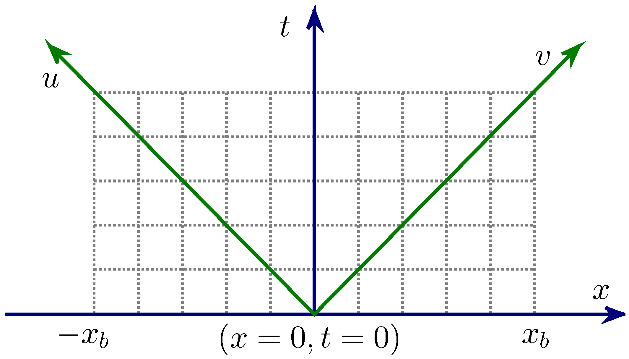
where σ and r are functions of the coordinates u and v. u and v are outgoing and ingoing characteristics (trajectories of photons), respectively. For convenience, in this paper, we use a slightly modified form described by Equation (26), obtained by defining and [51],
This set of coordinates is illustrated in Figure 1. Similar to the Schwarzschild metric, the Reissner-Nordström metric can be expressed in Kruskal-like coordinates [52] (also see References [26,27,50,53]). So for ease and intuitiveness, we set the initial conditions close to those of the Reissner-Nordström metric in Kruskal-like coordinates, taking into account the presence of a physical scalar field ψ, a scalar degree of freedom , and the potential .
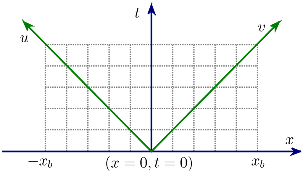
Figure 1.
Initial and boundary conditions for charge scattering. Initial slice is at . Definition domain for x is . and .
Figure 1.
Initial and boundary conditions for charge scattering. Initial slice is at . Definition domain for x is . and .
In the form of Reference [53], the Reissner-Nordström metric in Kruskal-like coordinates in the region of can be written as
where and are the locations and surface gravities for the outer and inner horizons of a Reissner-Nordström black hole, respectively. is defined implicitly below [53],
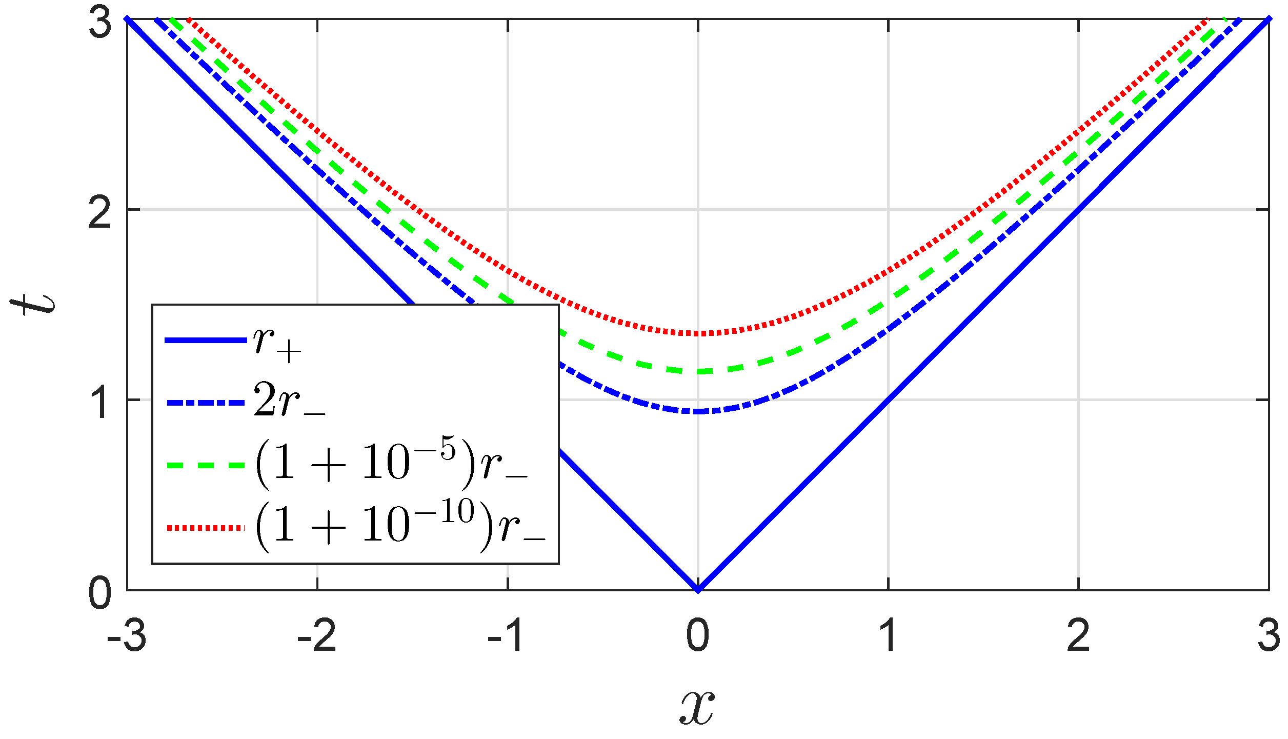
Some details for this set of coordinates are given in Appendix B. In this set of coordinates, as implied by Equation (28), the exact inner horizon is at regions where and are infinite. However, it is found that, even when and take moderate values, r still can be very close to the inner horizon, e.g., . (See Figure 2.) Therefore, at such regions, the interaction between the scalar fields and the inner horizon still can be very strong, then we can investigate mass inflation numerically.
This formalism has several advantages as follows:
- (1)
- In the line element Equation (26), one coordinate is timelike and the rest are spacelike. This is a conventional setup. It is more convenient and more intuitive to use this set of coordinates. For the set of coordinates described by Equation (25), in the equations of motion, many terms are mixed derivatives of u and v; while for the set of coordinates described by Equation (26), in the equations of motion, spatial and temporal derivatives are usually separated.
- (2)
- We set initial conditions close to those in the Reissner-Nordström metric. Consequently, with the terms related to the scalar fields being removed, we can test our code by comparing the numerical results to the analytic ones in the Reissner-Nordström case conveniently. Moreover, by comparing dynamics for scalar collapse to that in the Reissner-Nordström case, we can obtain intuitions on how the scalar fields affect the geometry.
- (3)
- The interactions between scalar fields and the geometry are local effects. In References [29,30], the space between the inner and outer horizons are compactified into finite space. This overcompactification, at least to us, makes it a bit hard to understand the dynamics. In the configuration that we choose, the space is partially compactified, and the picture of charge scattering turns out to be simpler.

Figure 2.
Contour lines for r defined by Equation (28) in a Reissner-Nordström geometry with and . Although the exact inner horizon is at regions where and are infinite, r can be very close to the inner horizon even when and take moderate values.
Figure 2.
Contour lines for r defined by Equation (28) in a Reissner-Nordström geometry with and . Although the exact inner horizon is at regions where and are infinite, r can be very close to the inner horizon even when and take moderate values.
2.4. Model
For a viable dark energy model, has to be positive to avoid ghosts [54], and has to be positive to avoid the Dolgov-Kawasaki instability [55]. The model should also be able to generate a cosmological evolution compatible with the observations [56,57] and to pass the Solar System tests [39,58,59,60,61,62,63]. Equivalently, general relativity should be restored at high curvature scale, and the model mainly deviates from general relativity at low curvature scale comparable to the cosmological constant. In this paper, we take a typical dark energy model, the Hu-Sawicki model, as an example. This model reads [39]
where n is a positive parameter, and are dimensionless parameters, , and is the average matter density of the current Universe. We consider one of the simplest versions of this model, i.e., ,
where D is a dimensionless parameter. In this model,
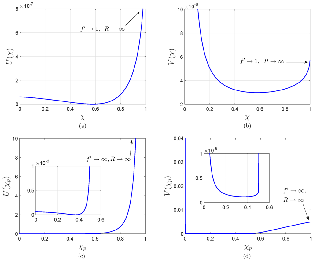
Figure 3.
Potentials for models. and . and are the potentials in the Jordan and Einstein frames and can be obtained from Equation (9) and Equation (23), respectively. (a) and (b) are for the Hu-Sawicki model Equations (30), , while (c) and (d) are for the combined model Equations (79), . , , and .
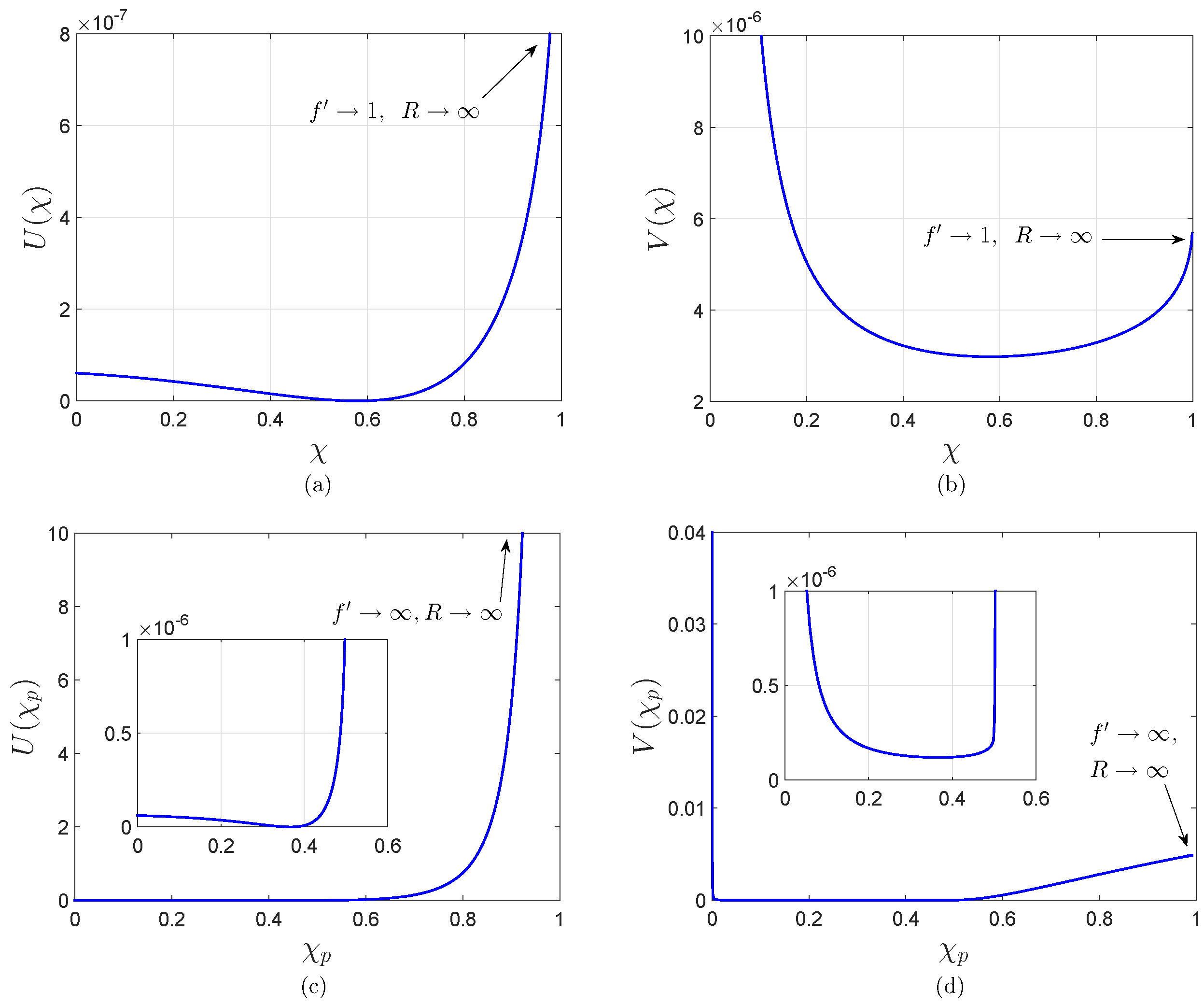
As implied in Equation (32), to make sure that the de Sitter curvature, for which , has a positive value, the parameter D needs to be greater than 1. In this paper, we set D to and set to or . Then, together with Equation (23) and Equation (32), these values imply that the radius of the de Sitter horizon is about . Moreover, in the configuration of the initial conditions described in Section 3.2 and Section 6, the radii of the outer apparent horizons of the formed black holes are about and , respectively. (See Figure 6f and Figure 11f). The potentials in the Jordan and Einstein frames are plotted in Figure 3a,b, respectively.
3. Numerical Setup for Charge Scattering
In this section, we set up the numerical formalisms for charge scattering in gravity, including field equations, initial conditions, boundary conditions, discretization scheme, and tests of numerical codes.
3.1. Field Equations
Details on the Einstein tensor and the energy-momentum tensor for a scalar field are given in Appendix C. In double-null coordinates Equation (26), using
one obtains the equation of motion for r,
where and other quantities are defined analogously. For simplicity, we define and integrate the equation of motion for η, instead [51]. The equation of motion for η can be obtained by rewriting Equation (33) as
provides the equation of motion for σ,
In double-null coordinates, the equations of motion for ϕ (21) and ψ (22) become, respectively,
where
The and components of the Einstein equations yield the constraint equations
Via the definitions of and , the constraint equations can be expressed in coordinates. Equations (40) − (39) and (40) + (39) generate the constraint equations for the and components, respectively,
3.2. Initial Conditions
We set the initial data to be time symmetric:
Therefore, in this configuration, the constraint Equation (41) is satisfied identically. Note that, in this configuration, the values of and at are the same as those in the Reissner-Nordström metric case.
We set the initial value for ψ as
In this paper, we give ϕ two sets of initial conditions:
where is de Sitter value, defined by . The initial value for σ is defined to be the same as the corresponding one in the Reissner-Nordström case described by Equation (27),
where r is defined by Equation (28) with . We obtain the initial value for r in charge scattering by combining Equations (33) and (42),
We set at the origin as in the Reissner-Nordström metric case. The definition domain for the spatial coordinate x is . Then can be obtained by integrating Equation (48) via the fourth-order Runge-Kutta method from to , respectively. The initial values of r, σ, , and ψ are shown in Figure 11.
In this paper, we employ the finite difference method. The leapfrog integration scheme is implemented, which is a three-level scheme and requires initial data on two different time levels. With the initial data at , we compute the data at with a second-order Taylor series expansion as done in Reference [64]. Take the variable ψ as an example,
The values of and are set up as discussed above, and the value of can be obtained from the equation of motion for ψ (37).
Up to this point, the initial conditions are fixed, with all the field equations being taken into account. The first-order time derivatives of r, σ, ϕ, and ψ at described by Equation (43) ensure that the constraint Equation (41) is satisfied. The equation for at expressed by Equation (48) implies that the constraint Equation (42) is satisfied. Computations of r, σ, ϕ, and ψ at via a second-order Taylor series expansion, as expressed by Equation (49) for the case of ψ, satisfy all the equations of motion.
Note that the region of is included in the initial conditions. This may not be physical. However, we are mainly interested in the interior dynamics of black holes, and then it is not important where the scalar field originally comes from. This setup makes it convenient for us to compare the results of charge scattering to the known solutions of the Reissner-Nordström geometry. Therefore, we use this setup as a toy model.
3.3. Boundary Conditions
The values of r, σ, ϕ, and ψ at the boundaries of are obtained via extrapolations. In fact, since we are mainly concerned with the dynamics around , the boundary conditions will not affect the dynamics in this region, as long as is large enough.
3.4. Discretization Scheme
In this paper, we implement the leapfrog integration scheme, which is second-order accurate and nondissipative. We let the temporal and spatial grid spacings be equal, .
The equations of motion for ϕ (36) and for ψ (37) are coupled. Newton’s iteration method is employed to solve this problem [64]. With the illustration of Figure 4, the initial conditions provide the data at the levels of “down” and “here”. We need to obtain the data on the level of “up”. We take the values at the level of “here” to be the initial guess for the level of “up”. Then, taking ψ as an example, we update the values at the level of “up” using the following iteration:
where is the residual of the differential equation for the function , and is the Jacobian defined by
We do the iterations for the coupled equations one by one, and run the iteration loops until the desired accuracies are achieved.
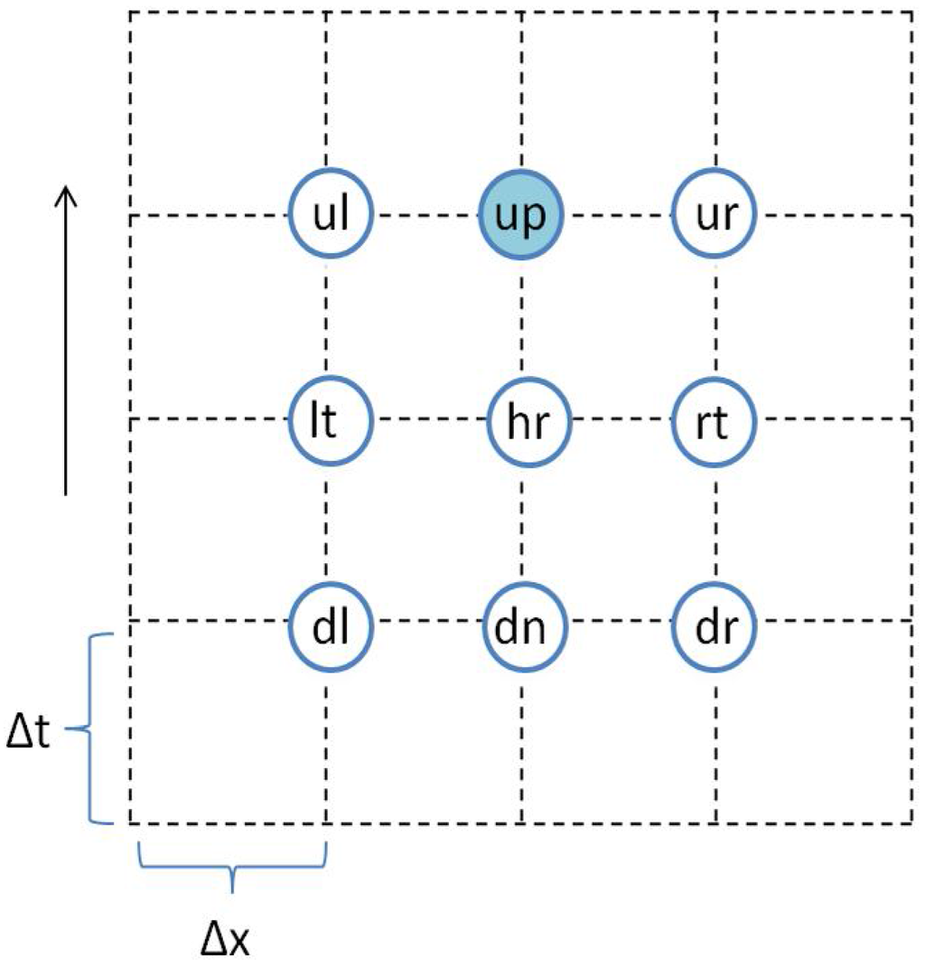
Figure 4.
Numerical evolution scheme.
Figure 4.
Numerical evolution scheme.

3.5. Tests of Numerical Code
To make sure that the numerical results are trustworthy, one needs to test the numerical code. We compare the numerical results obtained by the code with the analytic ones for the dynamics in a Reissner-Nordström geometry, and examine the convergence of the constraint equations and dynamical equations in charge scattering.
The dynamics in a Reissner-Nordström geometry is a special case for charge scattering, in which the contributions from the scalar fields are set to zero. This special case has analytic solutions expressed by Equations (27) and (28). Therefore, we can test our code by comparing the numerical and analytic results in the Reissner-Nordström geometry. Set , , and . We plot the evolutions of r and σ along the slice in Figure 5a. As shown in Figure 5a, numerical and analytic results match well at an early stage; while at a late stage where gravity and electric field become strong, the numerical evolutions have a time delay compared to the analytic solutions.
When the numerical results are obtained, we substitute the numerical results into the discretized equations of motion and the constraint equations, and find that they are well satisfied. See Figure 13 and Figure 15, for example. Moreover, the convergence of the constraint Equations (41) and (42) is examined. We assume one constraint equation is nth-order convergent: residual=, where h is the grid size. Therefore, the convergence rate of the discretized constraint equations can be obtained from the ratio between residuals with two different step sizes,
Our numerical results show that both of the constraint equations are about second-order convergent. As a representative, we plot the results for the constraint Equation (41) in Figure 5b for the slice .
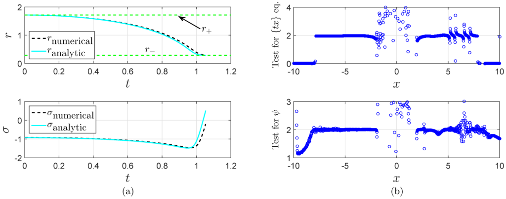
Figure 5.
Tests of numerical code for charge scattering. (a) Numerical vs analytic results for a Reissner-Nordström black hole. , , and . The slice is for . This is a special case of charge scattering with contributions of scalar fields being set to zero. Numerical and analytic results match well at an early stage, while at a later stage gravity and electric field become stronger, the numerical evolutions have a time delay, compared to analytic solutions; (b) Numerical tests for the constraint Equation (41) and the evolution of ψ on the slice . They are both second-order convergent.

Convergence tests via simulations with different grid sizes are also implemented [65,66]. If the numerical solution converges, the relation between the numerical solution and the real one can be expressed by
where is the numerical solution. Then, for step sizes equal to and , we have
Defining and , one obtains the convergence rate
The convergence tests for , σ, ϕ, and ψ are investigated. They are all second-order convergent. As a representative, the results for ψ are plotted in Figure 5b for the slice . The values of the parameters in charge scattering in this section are described at the beginning of Section 6. We use the spatial range of and the grid spacings of .
4. Neutral Scalar Collapse
In this section, we consider neutral collapse in flat geometry in gravity and discuss the mass inflation which happens in the vicinity of the central singularity of the formed black hole.
4.1. Numerical Setup
The numerical setup in neutral scalar collapse in gravity is discussed in Reference [20]. The dynamical equations for r, η, σ, ϕ, and ψ can be obtained by setting the terms related to the electric field in the corresponding equations in Section 3.1 to zero:
where .
In the equation of motion for σ (54), the term can create big errors near the center . To avoid such a problem, we use the constraint Equation (39) alternatively [51]. Defining a new variable g
one can rewrite Equation (39) as the equation of motion for g,
In the numerical integration, once the value of r at the advanced level is obtained, the value of σ at the current level will be computed using Equation (57).
We set the initial data as
The initial values for and are defined as
with , , , and . The parameters for the Hu-Sawicki model described by Equation (30) are set as and .
The local Misner-Sharp mass m is defined as [67]
(See Reference [68] for details on various properties of the Misner-Sharp mass/energy in spherical symmetry.) Then on the initial slice , the equations for r, m, and g are [20,51]
Set at the origin . Then the values of r, m, and g on the initial slice can be obtained by integrating Equations (63)–(65) from the center to the outer boundary via the fourth-order Runge-Kutta method. The values of r, σ, ϕ, and ψ at can be obtained with a second-order Taylor series expansion, as discussed in Section 3.2. The value of g at can be obtained using Equation (57).
The range for the spatial coordinate is defined to be . At the inner boundary , r is always set to zero. The terms in Equation (55) and in Equation (56) need to be regular at . Since r is always set to zero at the center, so is . Then we enforce ϕ and ψ to satisfy at . The value of g at is obtained via extrapolation. We set up the outer boundary conditions at via extrapolation. The temporal and the spatial grid spacings are .
The numerical code is second-order convergent and is the one developed in Reference [20].
4.2. Black Hole Formation
The evolutions of r, σ, ϕ, and ψ are plotted in Figure 6a–d, respectively. On the apparent horizon of a black hole, the expansion of the outgoing null geodesics orthogonal to the apparent horizon is zero [69]. Then in double-null coordinates, on the apparent horizon, there is [70]
Using this property, we locate the apparent horizon and plot it in Figure 6e–f. As shown in Figure 6a, the central singularity is also approached in the collapse. Therefore, a black hole is formed.
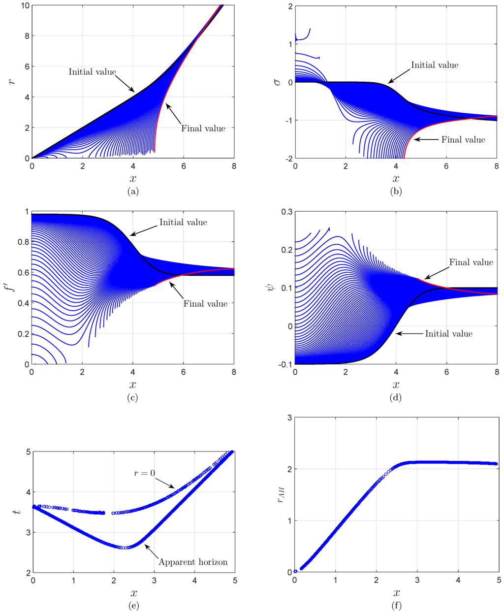
Figure 6.
Evolutions in neutral collapse for the Hu-Sawicki model Equation (30), . In (a)–(d), the time interval between two consecutive slices is . (e) and (f) are for the apparent horizon and the singularity curve of the formed black hole.
Figure 6.
Evolutions in neutral collapse for the Hu-Sawicki model Equation (30), . In (a)–(d), the time interval between two consecutive slices is . (e) and (f) are for the apparent horizon and the singularity curve of the formed black hole.

4.3. Asymptotic Dynamics in the Vicinity of the Central Singularity of the Formed Black Hole
We focus on the dynamics in the vicinity of the central singularity of the formed black hole. We will discuss that, in the vicinity of the singularity, due to the backreaction of the scalar fields on the geometry, the Misner-Sharp mass diverges. In other words, in addition to the inner horizons of Reissner-Nordström and Kerr black holes, mass inflation also happens in the vicinity of the central singularity of a Schwarzschild black hole.
In the vicinity of the central singularity, the field equation can be reduced to the following forms [20]:
The asymptotic solutions to Equations (67)–(69) are [20]
The variable ξ is defined as , where is the coordinate time on the singularity curve.
As implied in Equation (70), ψ is suppressed (magnified) by ϕ when is negative (positive). Due to the complex competition between gravity and dark energy, an approximate analytic expression for ψ is not obtained. Substituting Equation (71) into Equation (67) yields
Then we have
Using Equations (11) and (73), there is
So as shown in Figure 6c, when C is positive, χ also approaches zero as ξ and r approach zero. Then the transformation between the Jordan and Einstein frames, , breaks down. Actually this is not a serious problem, because numerical simulation stops anyway when the central singularity is approached. Moreover, in this paper, we discuss the dynamics in the vicinity of the central singularity rather than on the central singularity.
4.4. Mass Inflation
In the vicinity of the singularity, in the equation of motion for σ (68), because of the contribution from ϕ, is greater than the corresponding value in the Schwarzschild black hole case. This makes the mass function divergent near the singularity as will be discussed below.
Near the singularity, using Equation (62), Equation (71)–Equation (74), the mass function can be written as
where . In the Schwarzschild black hole case, . The mass function is always constant and is equal to the black hole mass. In neutral collapse, the parameter β does not change much and remains about . However, the parameter C is not zero. Then the metric quantity σ is modified. (See Equation (72)). As a result, the delicate balance between r and is broken. Consequently, as implied in Equation (76), near the singularity, the mass function diverges: mass inflation occurs.
During the collapse, before the black hole is formed, the energy of the scalar fields accumulates in the central region. As a result, the scalar fields near are stronger than those at large-x regions. Next we discuss three consequences. As a support, we examine the dynamics in the vicinity of the singularity via mesh refinement that was implemented in References [20,71], and plot two sample sets of results on the slices and in Figure 7 and Figure 8, respectively.

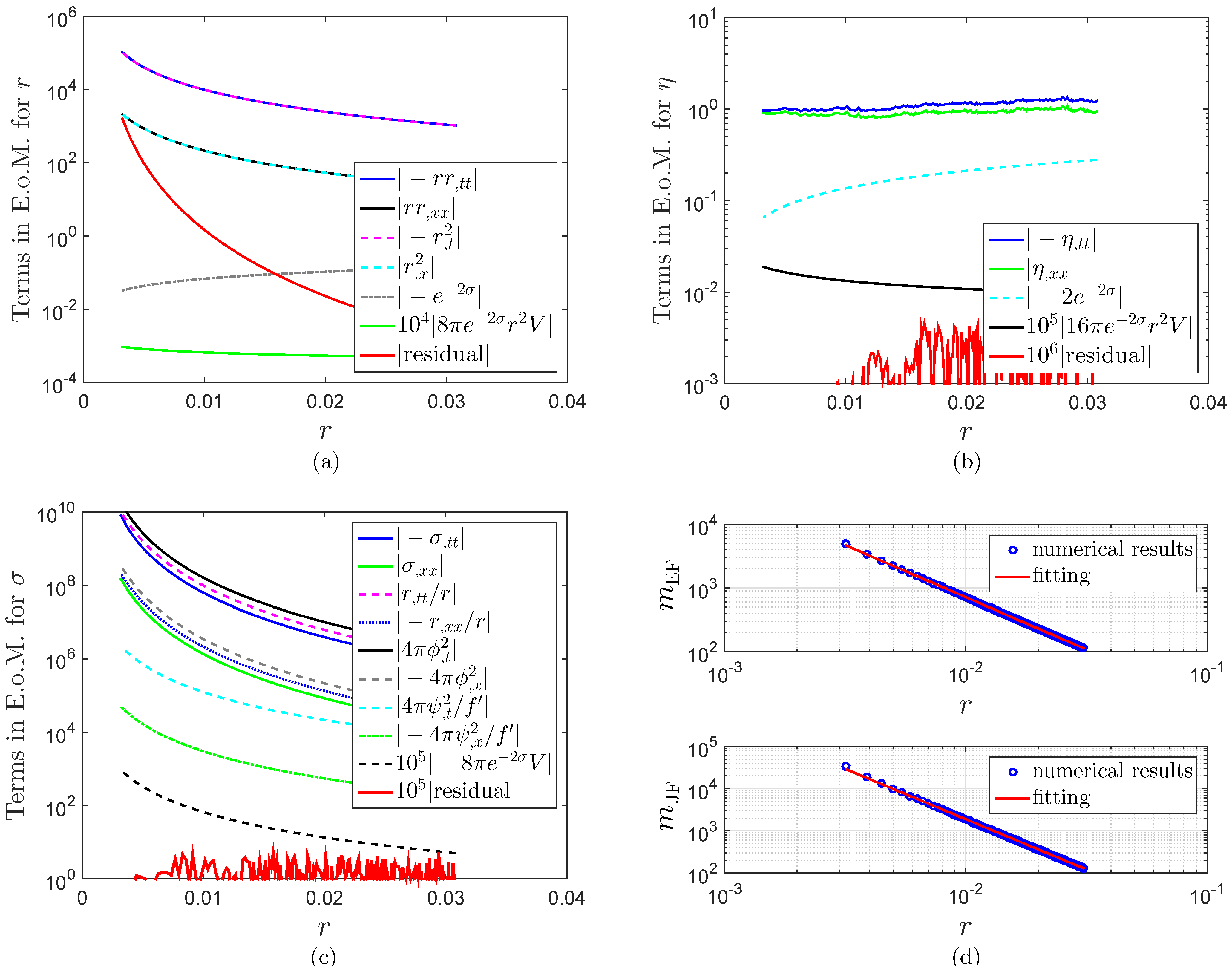
Figure 7.
(color online) Dynamics on the slice in neutral collapse for the Hu-Sawicki model Equation (30). (a)–(c): dynamical equations for r, η, and σ. (b) Near the central region, due to accumulation, the scalar field ϕ is strong. σ is positive. As a result, in the equation of motion for η (53), the terms and are negligible. The equation is reduced to . (d) , , . , , .
- (1)
- Values of σ. Due to the backreaction of the scalar fields on the geometry, σ in small-x regions is greater than in large-x regions. In fact, σ is positive in small-x regions, while negative in large-x regions. (See Figure 6b). Our numerical results of the parameter C in are at and at . Then we have and at , while and at . (See Equation (72)).
- (2)
- (3)
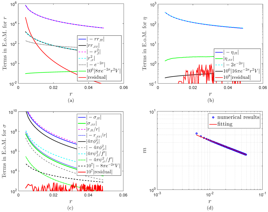
Figure 8.
(color online) Dynamics on the slice in neutral collapse for the Hu-Sawicki model. (a)–(c): dynamical equations for r, η, and σ. (b) At large-x regions, the scalar field ϕ is weak, and σ is negative. As a result, in the equation of motion for η (53), the term is important. The equation is reduced to . (d) , , .
Since gravity is defined in the Jordan frame, it is interesting to examine the mass function in the Jordan frame. A generalized Misner-Sharp energy in gravity in the Jordan frame was defined in Reference [40]. However, due to the complexity of some integrals, an explicit quasi-local form is usually not available with the exceptions of a Friedmann-Robertson-Walker universe and static spherically symmetric solutions with constant scalar curvature. In this paper, for simplicity, we remain to use the conventional format of the Misner-Sharp function. Considering the transformation that we used, , there are and . Considering that near the central singularity [20,41]
one can obtain that . Then the mass function in the Jordan frame can be written as
In the case of , due to the factor , is greater than . The along the slice is plotted in Figure 7d.
For stationary black holes (e.g., Schwarzschild and Reissner-Nordström), the Misner-Sharp mass function is always equal to the black hole mass. In spherical symmetry, at spatial infinity, the mass function describes the total energy/mass of an asymptotically flat spacetime [68]. In gravitational collapse case, it means the total mass of the collapsing system.
In the vicinities of the central singularity of a Schwarzschild black hole and the inner horizon of a Reissner-Nordström or Kerr black hole, the dynamics and some quantities are local. The mass function is just a parameter which varies at each point, not giving global information on the black hole mass.
5. Neutral Scalar Scattering
In this section, we consider neutral scattering, in which a neutral scalar field collapses in a Schwarzschild geometry in gravity. The numerical formalism is a simpler version of the one in charge scattering that has been constructed in Section 3, and it can be obtained by removing the electric terms in the field equations presented in Section 3.1 and replacing the Reissner-Nordström geometry with a Schwarzschild one.
5.1. A Dark Energy Singularity Problem
In neutral scattering, for usual initial conditions of the scalar degree of freedom , asymptotes to zero as the central singularity is approached, which is similar to what happens in the neutral scalar collapse discussed in Section 4. Details are skipped here. On the other hand, when the initial velocity or acceleration of is large enough, can become 1 before the central singularity is approached. As implied in Equation (29), for dark energy models, this means that the Ricci scalar becomes infinite, and the simulation breaks down. In this section, we will focus on this singular circumstance.
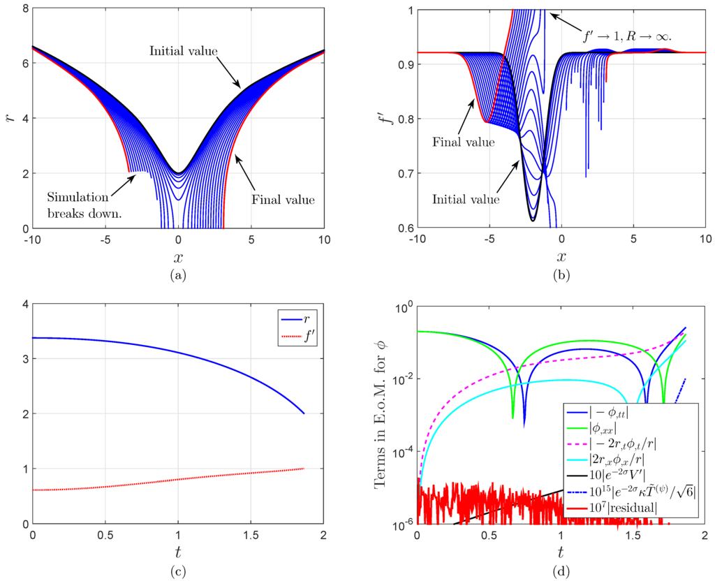
Figure 9.
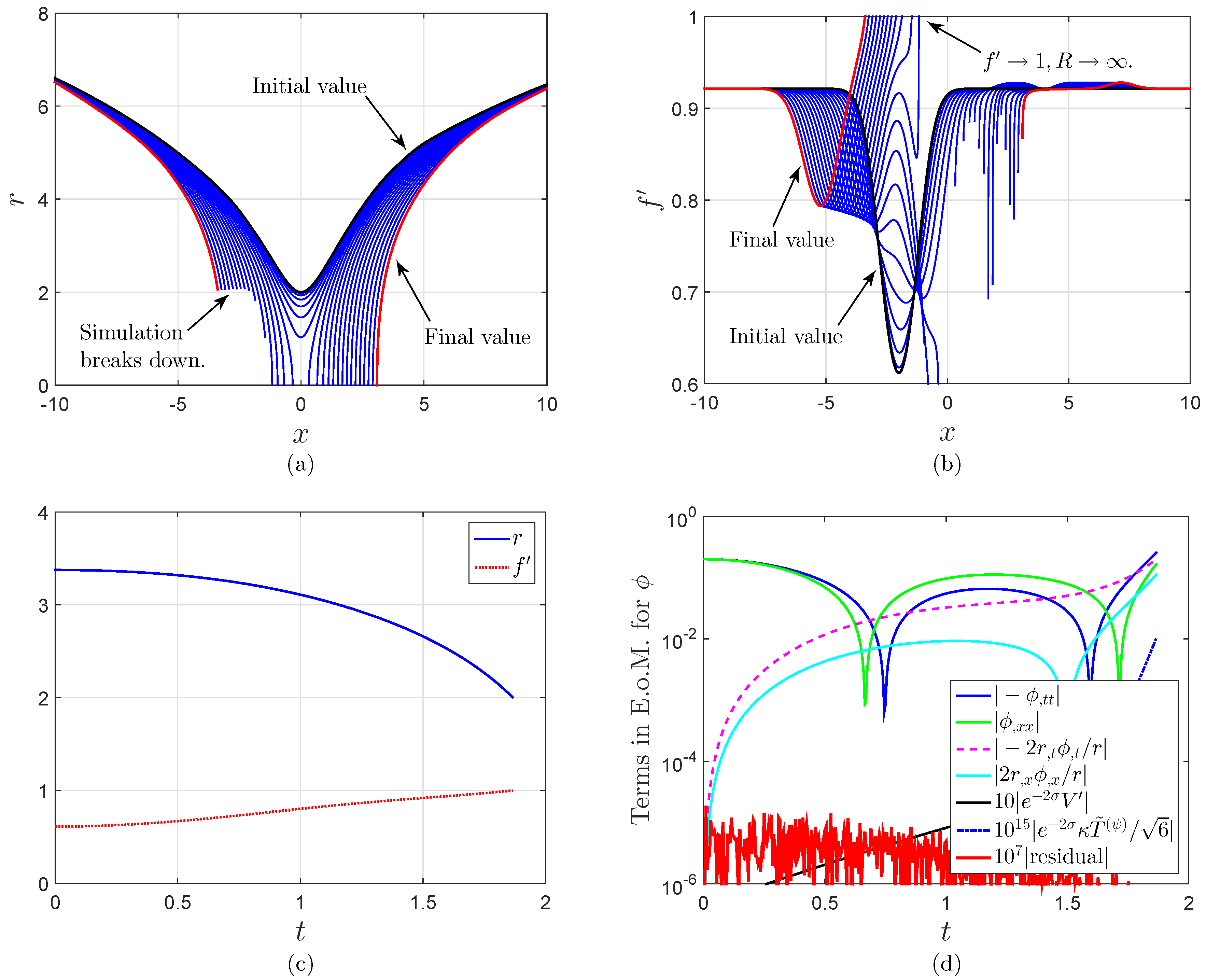
(color online) Results for neutral scalar collapse in a Schwarzschild geometry for the Hu-Sawicki model. (a) and (b): evolutions of r and . The time interval between two consecutive slices is . (c) evolutions of r and on the slice . (d) dynamical equation for ϕ on the slice . ϕ is mainly accelerated by the spatial derivative and the geometrical term . Eventually, ϕ and approach 0 and 1, respectively. Then the Ricci scalar becomes singularity, and the simulation stops.
Figure 9.
(color online) Results for neutral scalar collapse in a Schwarzschild geometry for the Hu-Sawicki model. (a) and (b): evolutions of r and . The time interval between two consecutive slices is . (c) evolutions of r and on the slice . (d) dynamical equation for ϕ on the slice . ϕ is mainly accelerated by the spatial derivative and the geometrical term . Eventually, ϕ and approach 0 and 1, respectively. Then the Ricci scalar becomes singularity, and the simulation stops.
The parameters are set as follows:
- (1)
- Schwarzschild geometry: .
- (2)
- Physical scalar field: , , , and .
- (3)
- model: , , and .
- (4)
- Scalar degree of freedom: , , , , and .
- (5)
- Grid. Spatial range: . Grid spacings: .
The results in this circumstance are plotted in Figure 9. We plot the dynamics of ϕ on the slice in Figure 9d, from which one can see that ϕ is mainly accelerated by the spatial derivative and the geometrical term . Eventually, ϕ and approach 0 and 1, respectively. Then the Ricci scalar becomes singularity, and the simulation stops, as shown in Figure 9a.
5.2. Avoidance of the Singularity Problem
In fact, it has been argued that such a singularity problem can also be caused in cosmology and compact stars [72]. This problem can be avoided by adding an term to the dark energy model [42,43,44,45,46,47,48,49]. In this paper, we add the term to the Hu-Sawicki model,
In this combined model, at high curvature scale, . So a singular R is pushed to regions where and ϕ are also singular. Then the singularity problem is avoided. The parameters take the same values as in the last subsection. In addition, the new parameter α in the model Equation (79) is set to 1.
The numerical results for neutral scattering for this modified model are plotted in Figure 10. As shown in Figure 10b, for this model, can cross 1 without difficulty. What are the limits that and R can reach? As shown in Figure 10d, as the central singularity is approached, there is

Figure 10.
(color online) Results for neutral scalar collapse in a Schwarzschild geometry in a combined model Equation (79). (a) and (b): evolutions of r and . The time interval between two consecutive slices is . (c) evolutions of r and on the slice . (d) dynamical equation for ϕ on the slice .
Figure 10.
(color online) Results for neutral scalar collapse in a Schwarzschild geometry in a combined model Equation (79). (a) and (b): evolutions of r and . The time interval between two consecutive slices is . (c) evolutions of r and on the slice . (d) dynamical equation for ϕ on the slice .
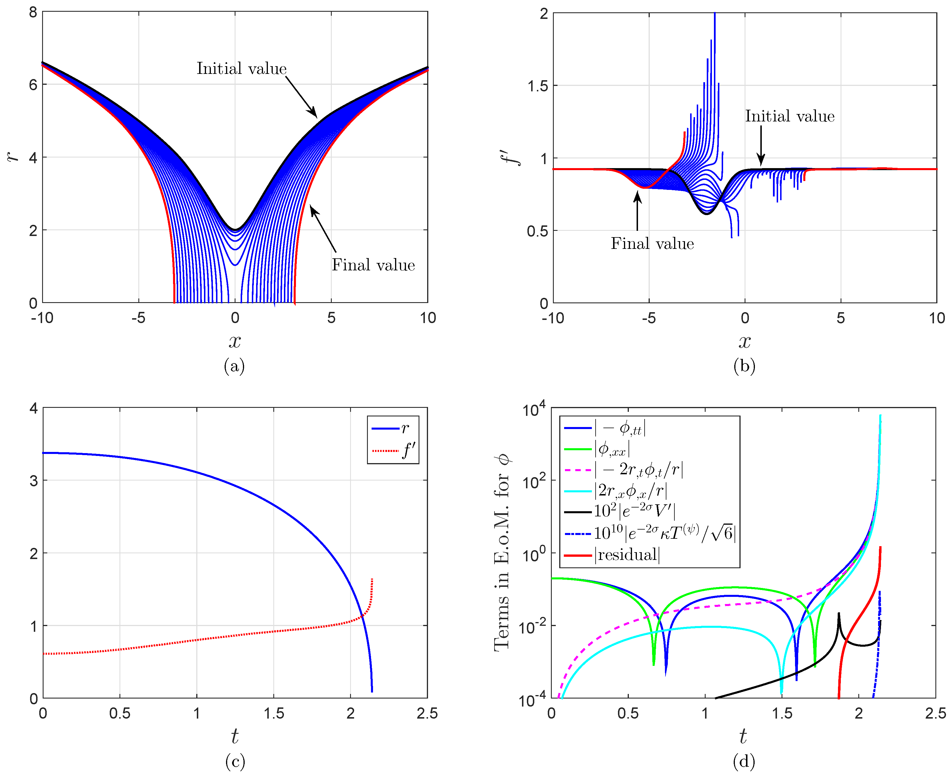
Since is negative, the above equation describes a positive feedback system of and : produces more of , and in turn produces more of . Since is positive, ϕ can be rapidly accelerated to positive infinity. Then and R will go to infinity as the central singularity is approached. This feature surely deserves some attention as discussed below.
The Starobinsky model, , was obtained by taking into account quantum-gravitational effects. It could cause inflation in the early Universe and is conventionally believed to be singularity-free [42]. The combined model is reduced to the Starobinsky model at high curvature scale. It is found that, in neutral scattering for the combined model, a new black hole, including a new central singularity, can be formed. Near the central singularity, gravity dominates other terms, including the potential related to the term, such that the Ricci scalar R can be pushed to infinity by gravity. We also simulate scalar collapse for the Starobinsky model in flat geometry. Similar results are obtained [73]. Therefore, the classical singularity problem, which is present in general relativity, remains in collapse for these models. Further details are skipped.
6. Results for Charge Scattering
In this section, we explore charge scattering: scalar collapse in a Reissner-Nordström geometry. We study the evolutions of the metric components and scalar fields and obtain approximate analytic solutions. We closely compare the dynamics in Schwarzschild black holes, Reissner-Nordström black holes, neutral scalar collapse, and charge scattering.
In this section, the parameters are set as follows:
- (1)
- Reissner-Nordström geometry: , and .
- (2)
- Physical scalar field: , , , and .
- (3)
- model: , , and .
- (4)
- Scalar degree of freedom: , with .
- (5)
- Grid. Spatial range: . Grid spacings: for Section 6.1 and Section 6.2, and for Section 6.3 and Section 6.4.
6.1. Evolutions
6.1.1. Outline
In this subsection, we describe the evolutions of r, σ, , and ψ that are plotted in Figure 11. Examining the equations of motion (33)–(37) and the numerical results plotted in Figure 13 and Figure 15, one can see that in the charge scattering dynamical system, there are three types of quantities as follows:
- (1)
- Metric components: r and σ. They contribute as gravity.
- (2)
- Scalar fields: ϕ and ψ. They contribute as self-gravitating fields.
- (3)
- Electric field and . As implied in Equation (33), they are repulsive forces. However, the numerical results show that in charge scattering, compared to the contributions from other quantities, the contribution from is negligible.
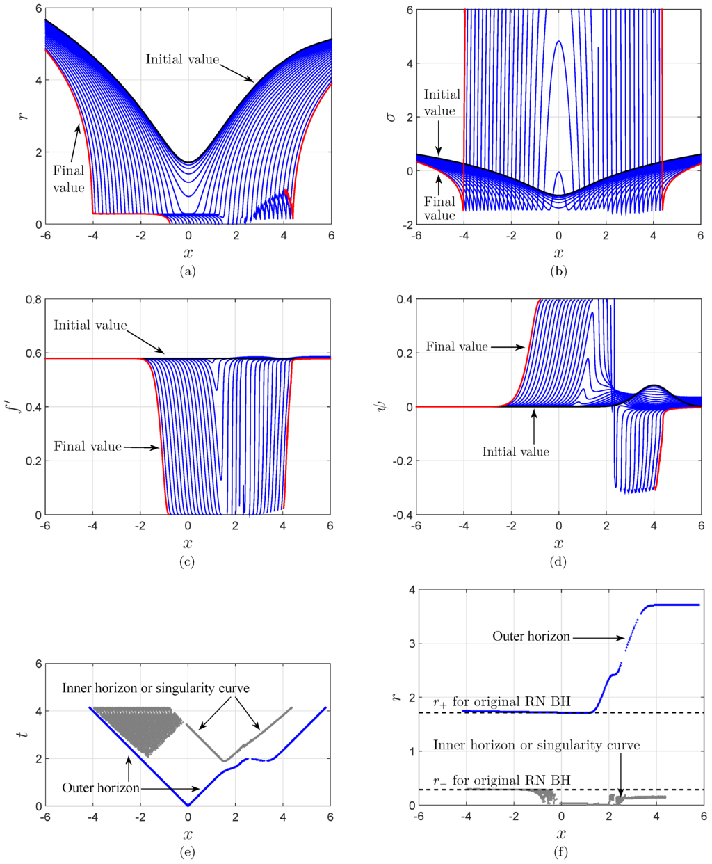
Figure 11.
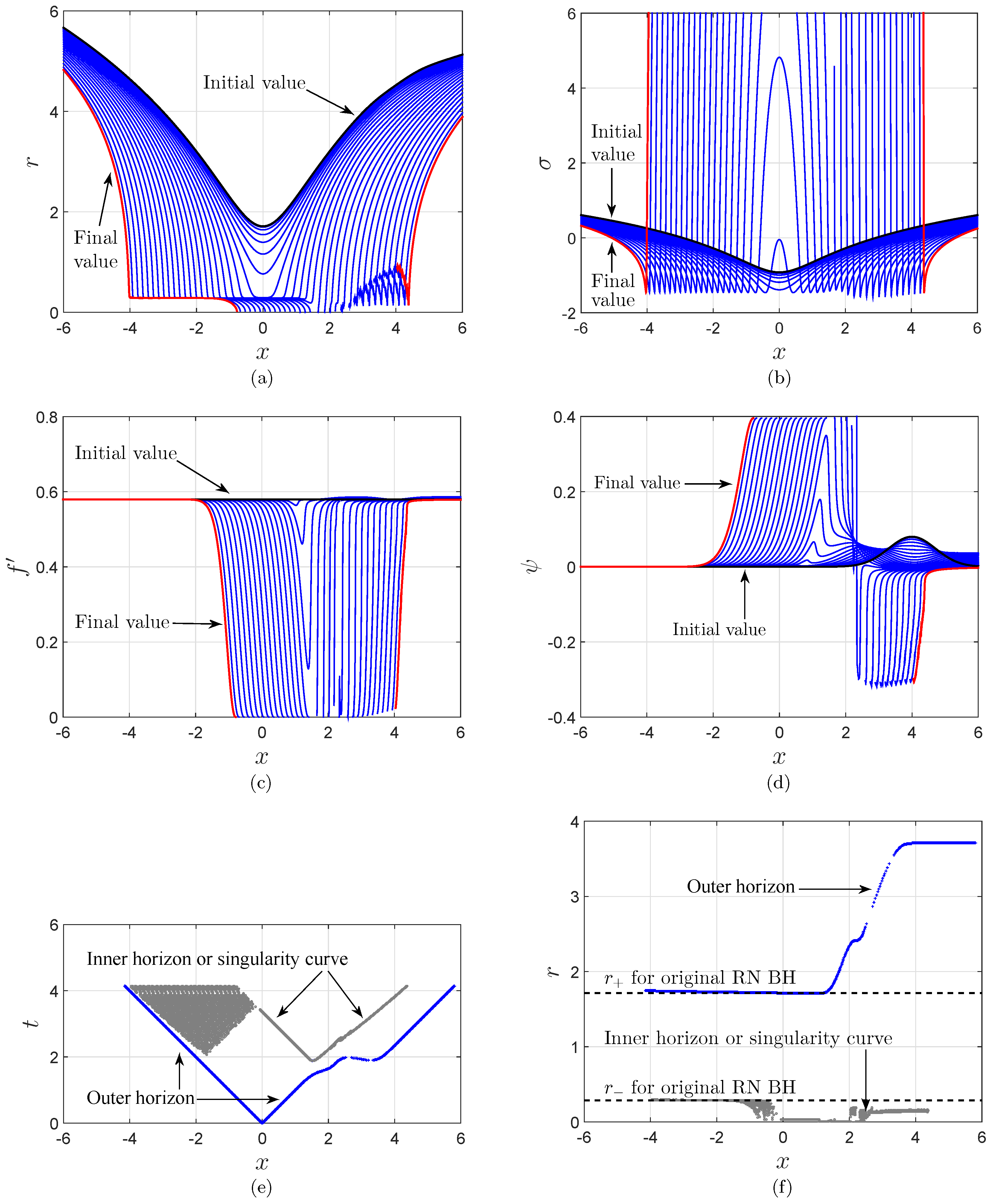
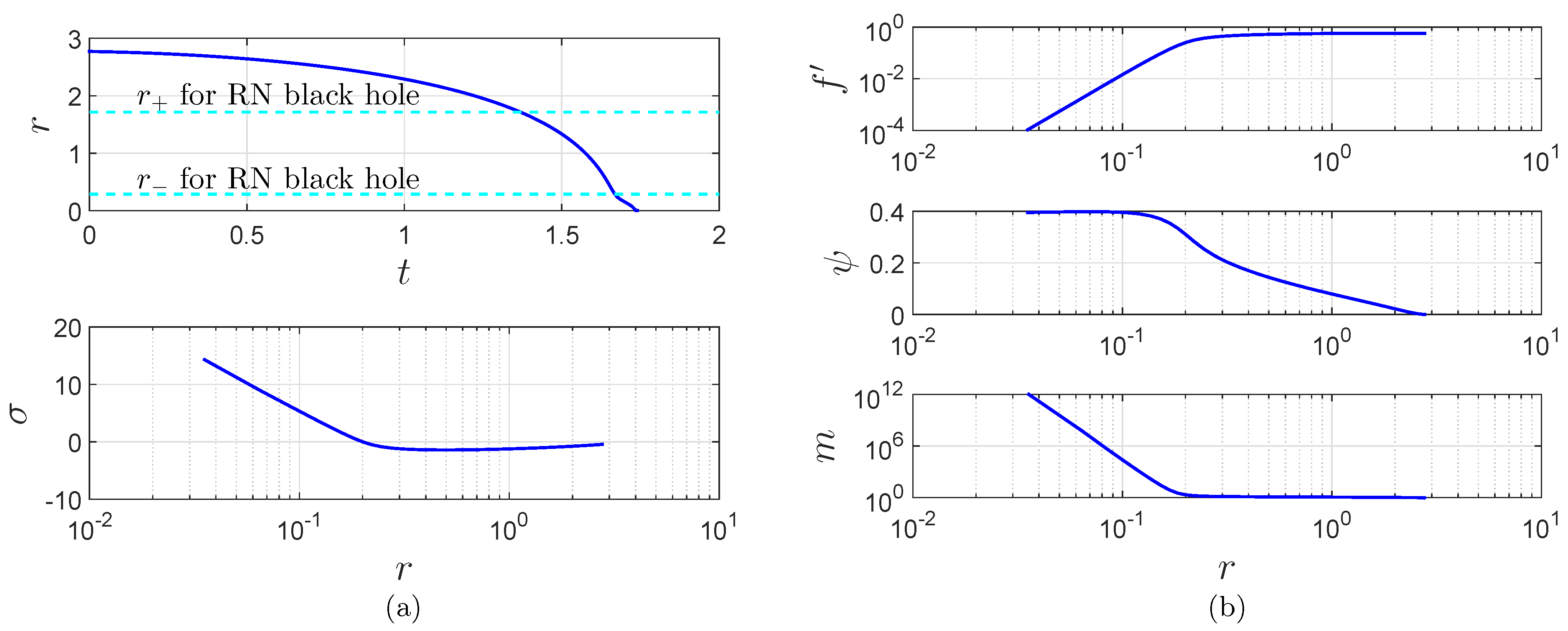
Evolutions in charge scattering. (a)–(d): evolutions of r, σ, , and ψ. The time interval between two consecutive slices is . (e) and (f) are for the apparent horizon and the singularity curve of the black hole. When the scalar field is strong enough (around ), the inner horizon can be pushed to the center, and the central singularity becomes spacelike. When the scalar field is weak enough (e.g., ), the inner horizon does not change much. At the intermediate state (e.g., ), the inner horizon contracts to zero, and the central singularity becomes null. The results for the inner horizon, especially for , are not that accurate. We are aware that the inner horizon is actually at infinity, while r still can be very close to when x and t take moderate values.
Figure 11.
Evolutions in charge scattering. (a)–(d): evolutions of r, σ, , and ψ. The time interval between two consecutive slices is . (e) and (f) are for the apparent horizon and the singularity curve of the black hole. When the scalar field is strong enough (around ), the inner horizon can be pushed to the center, and the central singularity becomes spacelike. When the scalar field is weak enough (e.g., ), the inner horizon does not change much. At the intermediate state (e.g., ), the inner horizon contracts to zero, and the central singularity becomes null. The results for the inner horizon, especially for , are not that accurate. We are aware that the inner horizon is actually at infinity, while r still can be very close to when x and t take moderate values.
Furthermore, these quantities can be separated into two sides: the gravitating side (r, σ, ϕ, and ψ) and the repulsive side [electric field and ]. The dynamics in charge scattering consists mainly of how these variables interact and how the gravitating and repulsive sides compete.
According to the strength of the scalar field, charge scattering can be classified into five types as follows:
- (1)
- Type I: spacelike scattering. When the scalar field is very strong, the inner horizon can contract to zero volume rapidly, and the central singularity becomes spacelike. Sample slice: in Figure 11. See Section 6.2.
- (2)
- Type II: null scattering. When the scalar field is intermediate, the inner horizon can contract to a place close to the center or reach the center. For each variable, the spatial and temporal derivatives are almost equal. In the case of the center being reached, the central singularity becomes null. This type has two stages: early/slow and late/fast. In the early stage, the inner horizon contracts slowly, and the scalar field also varies slowly. In the late stage, the inner horizon contracts quickly, and the dynamics is similar to that in the spacelike case. Sample slice: in Figure 11. See Section 6.3 and Section 6.4.
- (3)
- Type III: critical scattering. This case is on the edge between the above two cases. When the central singularity is reached, it becomes null. Sample slice: in Figure 11. Due to the similarity to that in general relativity discussed in Reference [41], details on this type of scattering in gravity are skipped in this paper.
- (4)
- (5)
- Type V: tiny scattering. When the scalar field is very tiny, the influence of the scalar field on the geometry is negligible. Sample slice: in Figure 11.
In this paper, we will discuss Types I, II, and IV.
6.1.2. Causes of Mass Inflation and Evolutions
The local Misner-Sharp mass for a charge black hole hole is
In a Reissner-Nordström geometry, in Kruskal-like coordinates expressed by Equation (27), near the inner horizon, although σ asymptotes to positive infinity, is much less than . Consequently, approaches zero. Then as implied in Equation (81), the mass function m takes a finite value and is equal to the black hole mass. For more details, see Reference [41].
In charge scattering, the equations of motion for and σ are
At the beginning, and may be less than and , respectively. However, as r decreases toward the central singularity, gravity becomes stronger. Then and become greater than and , respectively. (See Figure 15). As a result, in this case, the repulsive “force”, , is greater than the corresponding one, , in a Reissner-Nordström geometry. This makes σ accelerate faster than in the Reissner-Nordström geometry. Consequently, the repulsive force from for is much weaker than the corresponding value in the Reissner-Nordström geometry. As a result, near the inner horizon, is much greater than the corresponding one in the Reissner-Nordström case. Then moves from extremely tiny values in the Reissner-Nordström metric case to moderate values, and r crosses the inner horizon for the given Reissner-Nordström geometry. With Equation (81), the mass parameter grows dramatically: mass inflation takes place. In other words, regarding the causes of mass inflation in charge scattering, the scalar fields’ backreaction on r is more important than that on σ. The evolutions of r, σ, , and ψ are plotted in Figure 11a–d.
Because of gravity from the black hole and the contribution from the physical scalar field, for some configurations, can decrease to zero as the central singularity is approached. (See Equation (36) and Figure 11, Figure 13, and Figure 15). Nothing is wrong with this circumstance. However, for certain configurations, can be pushed to 1, as shown in Figure 21. Correspondingly, the Ricci scalar R becomes singular. We will discuss the former case in this section and the latter case in Section 8.
The evolution of ψ is plotted in Figure 11d. In the configurations that we consider, as the central singularity is approached, because of the strong suppression from the dark energy scalar ϕ, ψ asymptotes to constant values.
6.1.3. Locations of Horizons
We locate the outer and inner horizons using the following equation,
The results are plotted in Figure 11e,f. Due to the absorptions of the energies of ϕ and ψ, the outer horizon increases from the original value of to . Note that the results for the inner horizon, especially at regions where , are not that accurate. We are aware that the inner horizon is actually at infinity, while r still can be very close to even when x and t take moderate values.
6.2. Spacelike Scattering
In spacelike scattering, the scalar field is so strong, such that the inner horizon can contract to zero volume rapidly, and the central singularity converts from timelike into spacelike. Taking the slice as an example, we plot the evolutions of r, σ, , ψ, and m on this slice in Figure 12. The mass function remains equal to the mass of the original Reissner-Nordström black hole, , until r is very close to . By then mass inflation takes place. We examine the dynamics near the central singularity via mesh refinement and plot the terms in the dynamical equations in Figure 13.
The strongness of the scalar field causes several consequences as below.
- (1)
- Motion of r. The quantity r does not decelerate much when it crosses the inner horizon of the given Reissner-Nordström black hole, and it can approach the center. (See Figure 12).
- (2)
- Nature of the central singularity. The central singularity converts from timelike into spacelike.
- (3)
- The dynamics in spacelike scattering is similar to that in strong, neutral scalar collapse. The quantity σ takes large positive values, such that in the vicinity of the central singularity, compared to other terms, the term in the equation for r Equation (33) and the term in the equation for σ Equation (35) are negligible. As a result, in the vicinity of the central singularity, the dynamics is similar to that in strong, neutral scalar collapse as expressed by Equations (67)–(70). (See Figure 7 and Figure 13). Then the quantities r, σ, ϕ, and m take similar forms as those in neutral collapse. (See Figure 14).In both strong, neutral scalar collapse and spacelike scattering, the equation of motion for η is reduced to . (See Figure 7b and Figure 13b).Since is negative, the term in Equation (37) functions as a friction force for ψ. Consequently, compared to ϕ, ψ grows slowly. As the singularity is approached, ψ even approaches constant values. (See Figure 14c,d). As shown in Figure 13e, near the singularity, two major sets of terms can be expressed asAlternatively,
- (4)
- Growth of mass function.In spacelike scattering, the equation of motion for ϕ can be simplified asConsequently, with the results obtained in Section 4.3, σ has the following asymptotic solution:with . Then similar to the mass function Equation (76) in neutral collapse, with Equaution Equation (81), the mass function in spacelike scattering can be written asNumerical results show that, for the sample slice , near the central singularity, the slope of the singularity curve K is about . As shown in Figure 14d, we linearly fit the numerical results of m viaobtainingFitting numerical results for σ according to Equation (87) and combining Equations (88) and (89), we obtainSimilarly, fitting numerical results for ϕ according to , we obtainOne can see that the above three sets of results match well.

Figure 12.
Evolutions along the slice in one spacelike scattering process. (a) evolutions of r and σ. (b) evolutions of , ψ, and m. In this case, the scalar fields are so strong, such that r can rapidly cross the line of and approach zero. Other variables (σ, , ψ, and m) also evolve rapidly after r has crossed the line of .
6.3. The Late/fast Stage of Null Scattering
When the scalar fields are less strong, the inner horizon may still contract to zero. However, in this case, the central singularity becomes null rather than spacelike. The equations of motion remain null: they have similar forms as free wave equations, e.g., .
In the Reissner-Nordström black hole case, near the center, the repulsive (electric) force dominates gravity, and the central singularity is timelike. In spacelike scattering as discussed in the last subsection, gravity from the scalar field and the background geometry dominates the repulsive force. As a result, the central singularity is spacelike. At the late stage of null scattering that will be studied in this subsection, the scalar field is less strong, and the central singularity is null. Because of this, one may say that null scattering is a critical case of the competition between repulsive and gravitational forces, in which case the two types of forces have a balance.

Figure 13.
(color online) Dynamics along the slice near the spacelike, central singularity. Near the singularity, we can approximately rewrite the original equations of motion for r, η, σ, ϕ, and ψ as follows. (a) . (b) . (c) . (d) . (e) and . Then we have .
Figure 13.
(color online) Dynamics along the slice near the spacelike, central singularity. Near the singularity, we can approximately rewrite the original equations of motion for r, η, σ, ϕ, and ψ as follows. (a) . (b) . (c) . (d) . (e) and . Then we have .
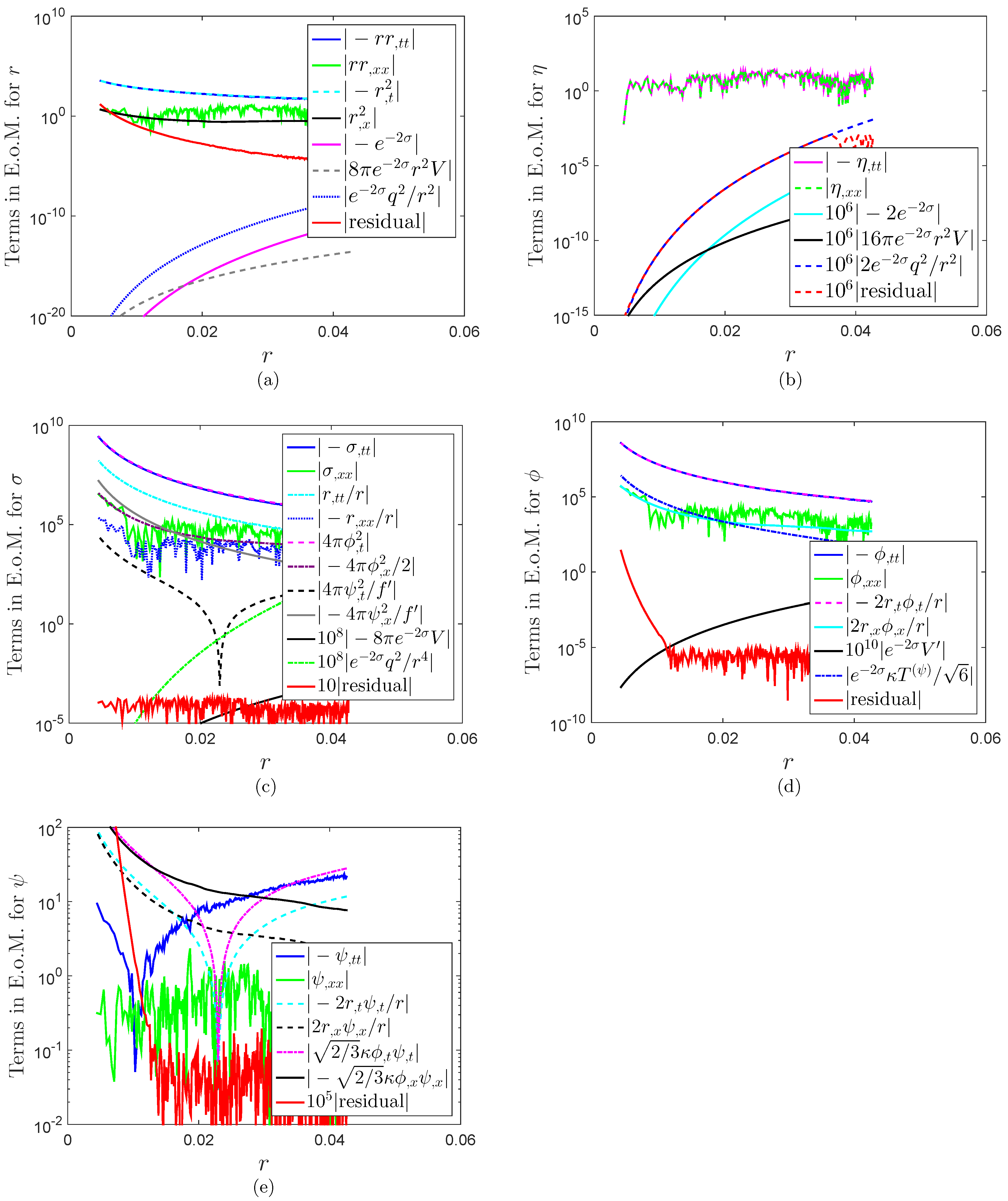

Figure 14.
Solutions along the slice near the spacelike, central singularity. (a) , , . , , . (b) , , . , , . (c) and (d): asymptotes to constant values as the central singularity is approached.
Figure 14.
Solutions along the slice near the spacelike, central singularity. (a) , , . , , . (b) , , . , , . (c) and (d): asymptotes to constant values as the central singularity is approached.
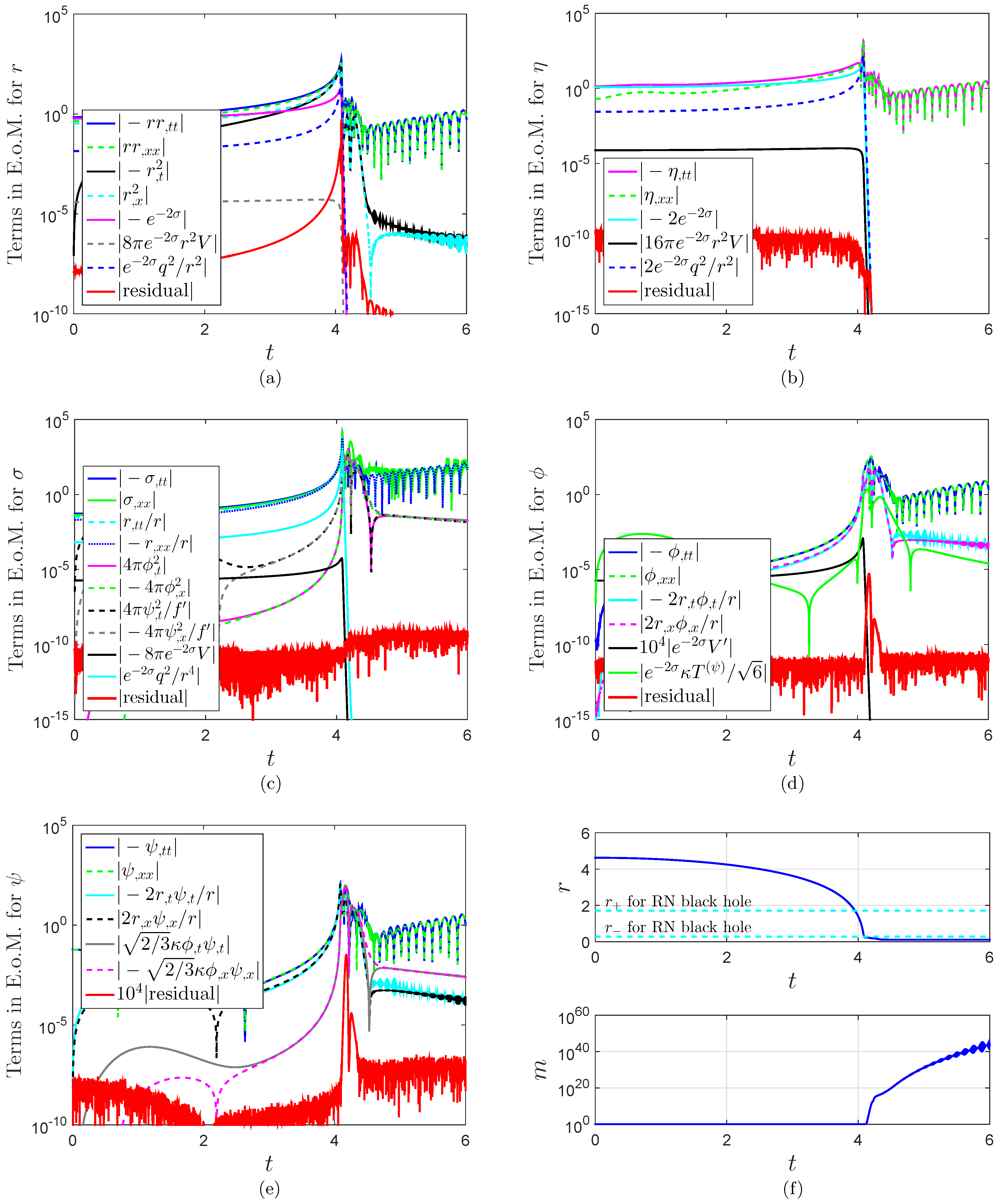
Take the slice as a sample slice, we plot the terms in the field equations for r, σ, ϕ, and ψ in Figure 15, and the evolutions of r, σ, ϕ, ψ, m, and in Figure 16. We investigate the dynamics in the vicinity of the central singularity via mesh refinement and plot the results in Figure 17.
The null scattering has two stages: early/slow and late/fast. As shown in Figure 15 and Figure 16, at the beginning of charge scattering, because of the repulsive force from the electric field, r, σ, ϕ, and ψ evolve slowly. As a result, the mass function m also grows slowly. We call this stage the early/slow stage. Later on, as the center is approached, gravity becomes very strong. Then these quantities evolve faster. We call this stage the late/fast stage.
As shown in Figure 15, when r is very small, the equations of motion for r (33), σ (35), and ϕ (36) can be rewritten as
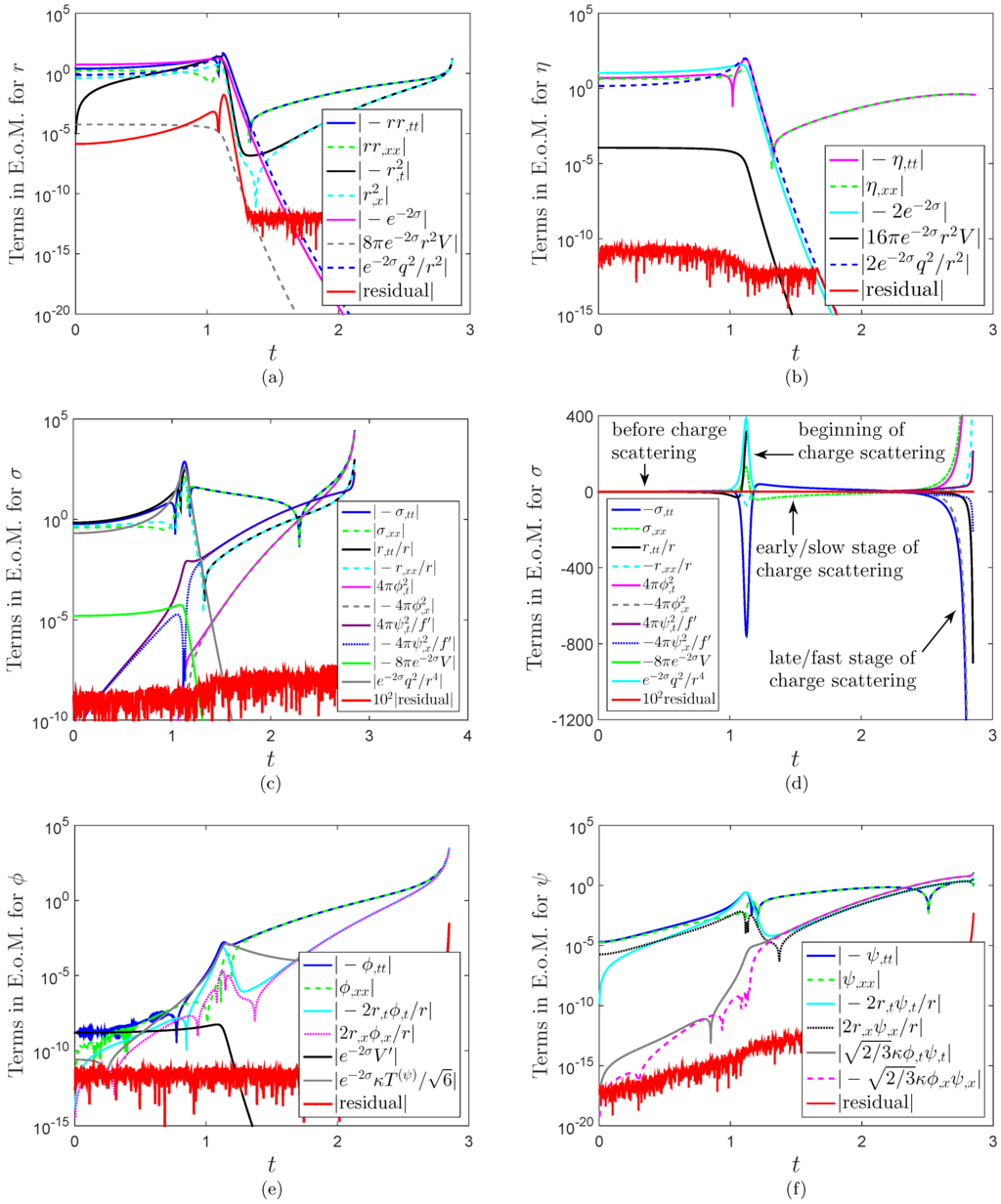
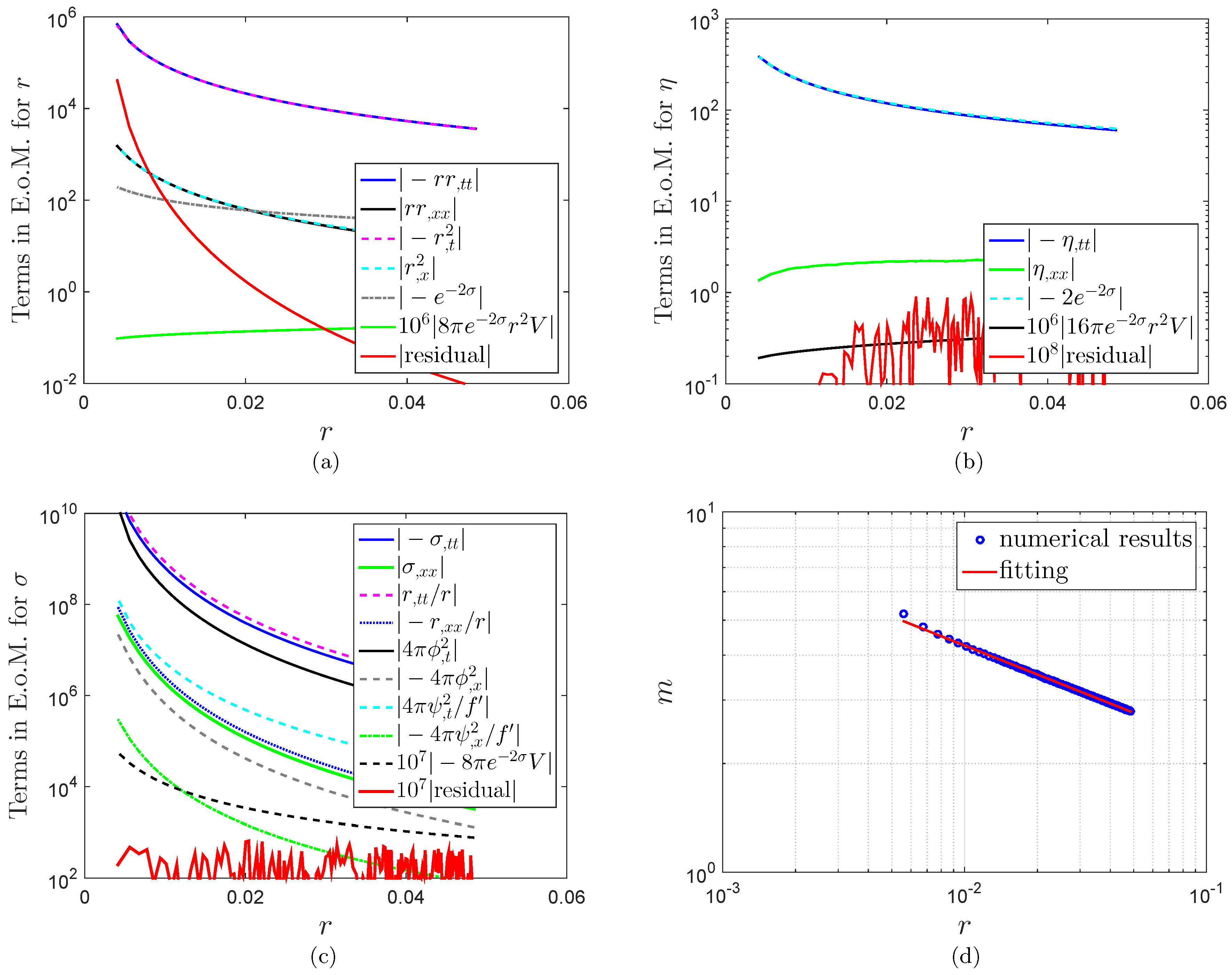
Figure 15.
(color online) Dynamics along the slice in null scattering. (a)–(f): dynamical equations for r, η, σ, ϕ, and ψ.
Figure 15.
(color online) Dynamics along the slice in null scattering. (a)–(f): dynamical equations for r, η, σ, ϕ, and ψ.

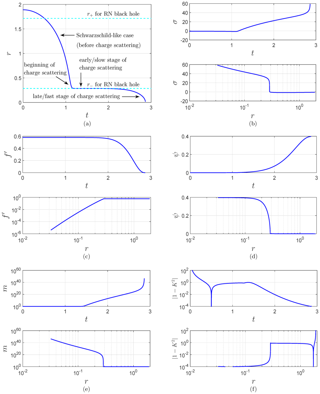
Figure 16.
Evolutions along the slice in null scattering. (a)–(f): evolutions for r, σ, f, ψ, m, and . At the early stage of mass inflation, , r varies slowly; while at the late stage, , r varies rapidly toward zero.
Figure 16.
Evolutions along the slice in null scattering. (a)–(f): evolutions for r, σ, f, ψ, m, and . At the early stage of mass inflation, , r varies slowly; while at the late stage, , r varies rapidly toward zero.
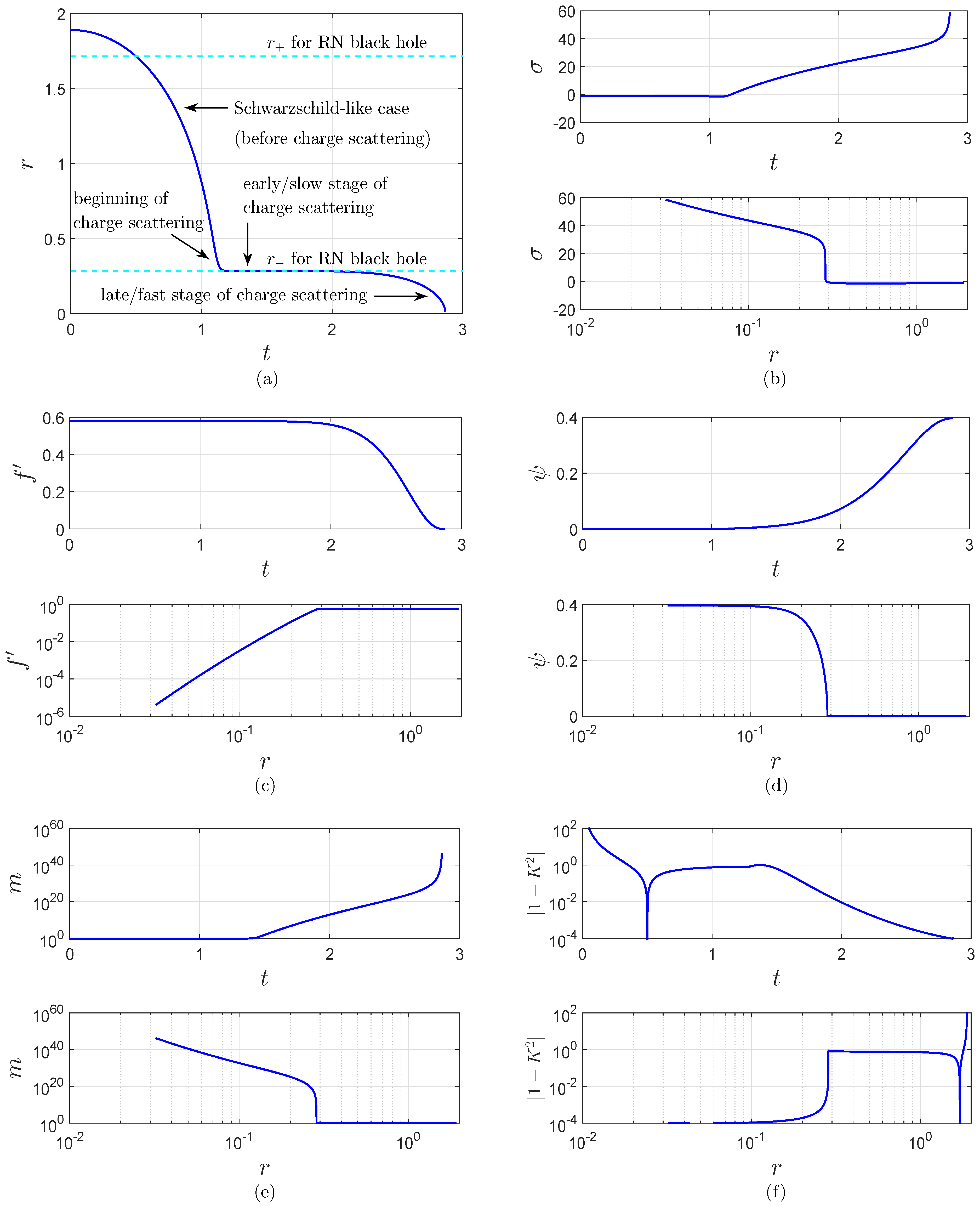
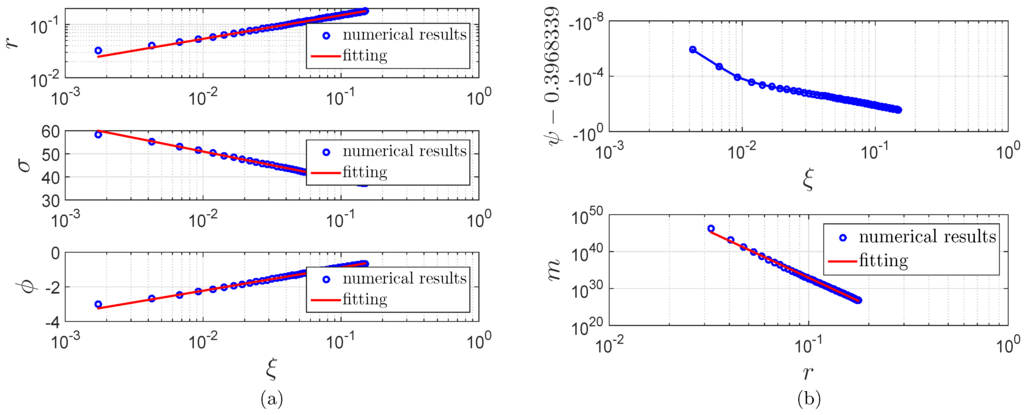
Figure 17.
Solutions near the null central singularity along the slice in null scattering. (a) , , . , , . , , . (b) ψ approaches a constant value . , , .
Figure 17.
Solutions near the null central singularity along the slice in null scattering. (a) , , . , , . , , . (b) ψ approaches a constant value . , , .

Since the above three equations have some similarities to the corresponding ones in spacelike scattering, it is natural to guess that the quantities r, σ, ψ, and m may have expressions similar to those in spacelike scattering. In fact, this guess is verified by the numerical results plotted in Figure 17. Then we have
As shown in Figure 16f, at the late stage, is around . Due to the similarity to spacelike scattering that we discussed in the last subsection, a comparison between numerical and analytical results for the fast stage of null scattering is skipped.
6.4. The Early/slow Stage of Null Scattering
As shown in Figure 15, at the early/slow stage of null scattering, the equations of motion for r (33), σ (35), ϕ (36), and ψ (37) are reduced as follows:
The above equations are like free scalar wave equations in flat spacetime. The derivatives of one variable (r, σ, ϕ, and ψ) are independent from the derivatives of another. Arbitrary functions of or can satisfy the above equations, and in principle, the initial conditions right after the collision between the scalar fields and the inner horizon will decide which function each variable can take. On the other hand, we find that, as shown in Figure 18, the constraint Equations (41) and (42) provide some useful information on the connections between some variables at the early stage of charge scattering:
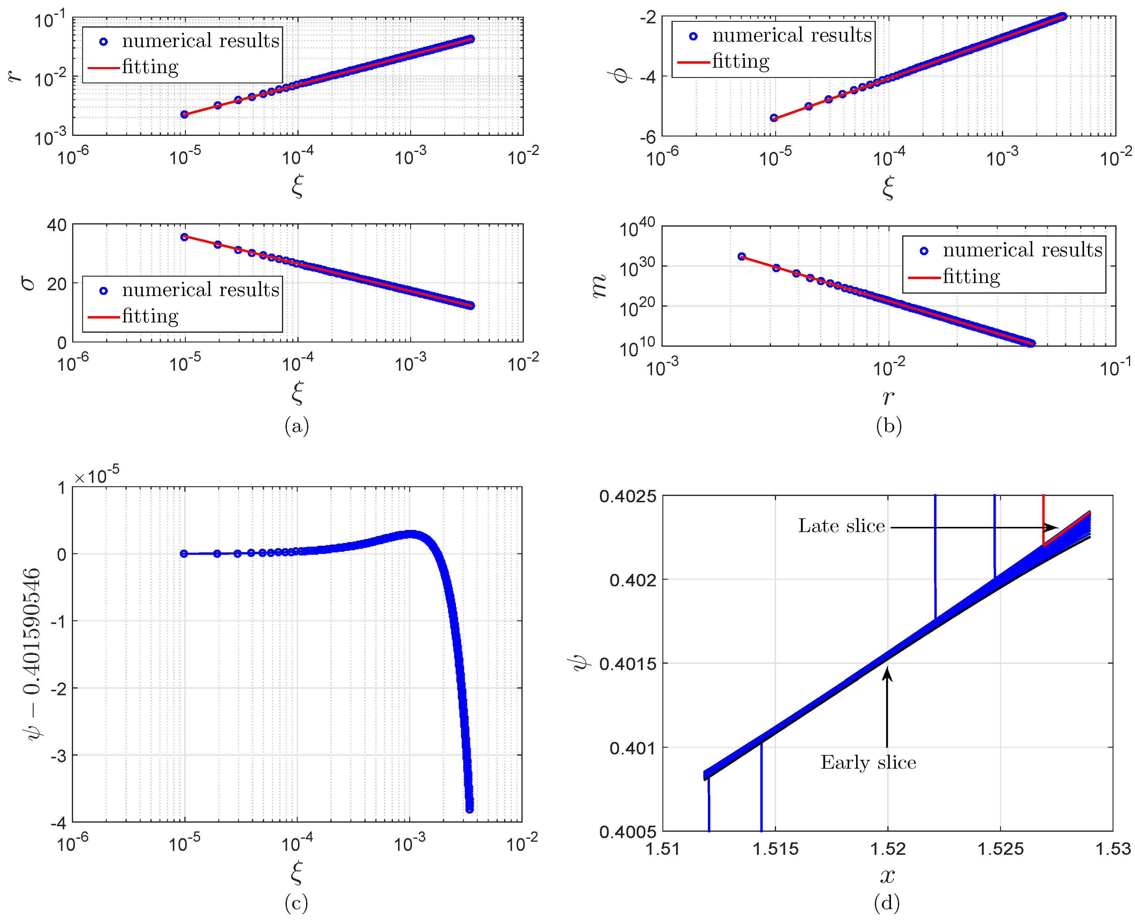
As shown in Figure 16, the quantities r, σ, , ψ, , and m change dramatically at the beginning of charge scattering where . Note that, near the central singularity, r, σ, and have approximate analytic expressions in terms of , where is the time coordinate of the singularity curve. So it is natural to guess that, at the early stage of charge scattering, the above quantities may also have approximate analytic expressions of , where is a certain time value related to the early stage of charge scattering. We plot the evolutions of these quantities at the early stage of charge scattering in Figure 18, from which one can see that r, , and σ may have the following approximate analytic expressions:
In fact, a logarithmic expression for σ is supported by its behavior near the inner horizon in the Reissner-Nordström black hole case. From Equations (28) and (47), one obtains that, as r approaches the inner horizon , in the case of , σ can be approximated by a logarithmic function of t. As shown in Figure 15c, describing the terms in the equation of motion for σ in charge scattering, at the very early stage () of the collision between the scalar fields and the inner horizon, compared to those from other terms, the contributions from the terms related to ϕ and ψ are tiny. Therefore, at this stage, the evolution of σ should not be much different from the corresponding one in the Reissner-Nordström geometry.
As shown in Figure 18c,d, ϕ and ψ can be well fitted by power law functions of ζ. Take ϕ as an example,
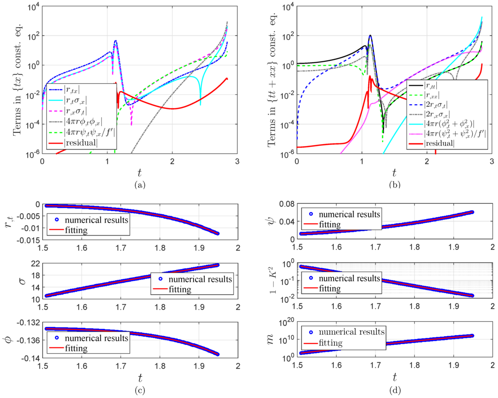
Figure 18.
(color online) Constraint equations and solutions along the slice at the early/slow stage of null scattering. (a) and (b): constraint Equations (41) and (42). (c) , , , , . , , , . , , , , . (d) , , , , . , , . , , , .
Figure 18.
(color online) Constraint equations and solutions along the slice at the early/slow stage of null scattering. (a) and (b): constraint Equations (41) and (42). (c) , , , , . , , , . , , , , . (d) , , , , . , , . , , , .

Currently we do not have derivations for this linear relation. The good thing is that, in the mass function, is a minor factor. Therefore, as verified in Figure 18d, the mass function can be reduced to
where a, b, λ, and are defined in Equations (103) and (104).
We list the fitting results below:
- (1)
- , , , , .
- (2)
- , , , .
- (3)
- , , , , .
- (4)
- , , , , .
- (5)
- , , .
- (6)
- , , , .
7. Weak Scalar Charge Scattering
In this section, we consider charge scattering with a weak scalar field. Parameter settings in this section are almost the same as those in the last section with the following exceptions:
- (1)
- Physical scalar field: , , , and .
- (2)
- Grid. Spatial range: . Grid spacings: .
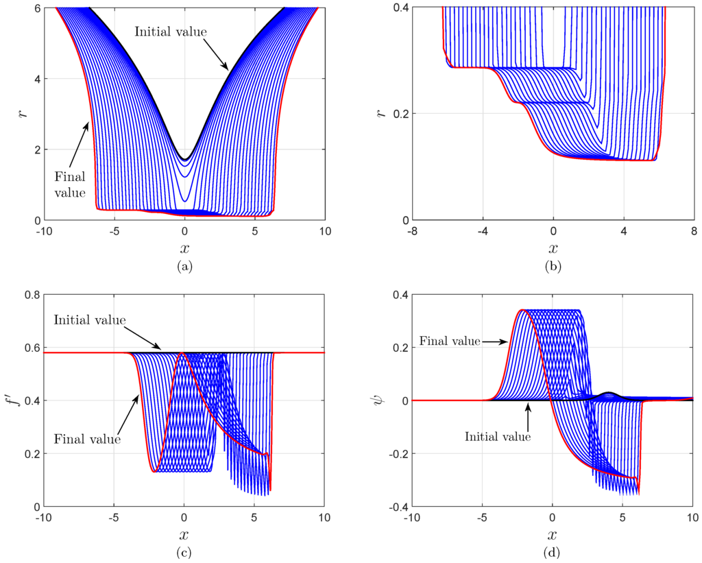
Figure 19.
Evolutions for charge scattering with a weak scalar field. (a)–(d): evolutions for r, , and ψ. The time interval between two consecutive slices is . The central singularity is not approached.
Figure 19.
Evolutions for charge scattering with a weak scalar field. (a)–(d): evolutions for r, , and ψ. The time interval between two consecutive slices is . The central singularity is not approached.

As discussed in the above section, in some spacetime regions where the scalar field is strong, the inner horizon can contract to zero volume, and the central singularity becomes spacelike. However, this does not always necessarily happen. After all, it takes energy for the inner horizon to contract. When the scalar field carries less energy, the inner horizon may only contract to a nonzero value. This is confirmed by our numerical results plotted in Figure 19. The evolution of σ is similar to that in strong scalar field case and is skipped. These results are in agreement with the mathematical proof in Reference [23] and the numerical work in Reference [34]. Since in this case the inner horizon is not totally destructed, one needs to reconsider whether the strong cosmic censorship conjecture is valid here. In addition, in Reference [74], it was argued that, when Hawking radiation is taken into account, this censorship may also be violated. Note that in Reference [75] the interior of a Schwarzschild black hole was also discussed with the backreaction from the Hawking radiation being taken into account.
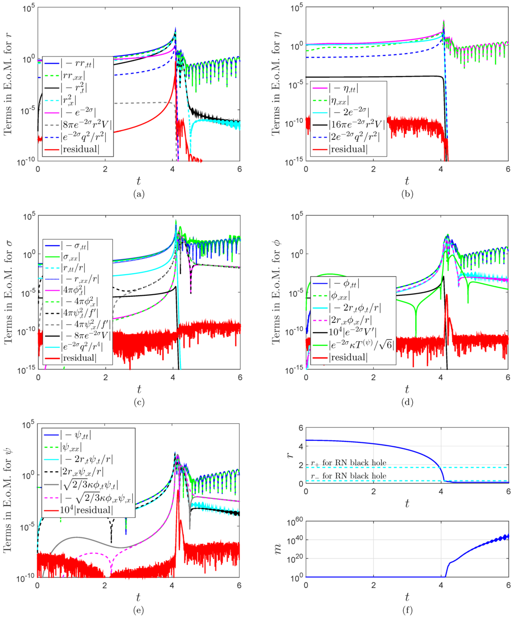
Figure 20.
(color online) Dynamics and evolutions on the slice in weak scattering. (a)–(e): dynamical equations for r, η, σ, ϕ, and ψ. (f) evolutions of r and m.
Figure 20.
(color online) Dynamics and evolutions on the slice in weak scattering. (a)–(e): dynamical equations for r, η, σ, ϕ, and ψ. (f) evolutions of r and m.
The dynamics for the quantities r, η, σ, ϕ, and ψ are plotted in Figure 20a–e, respectively. The numerical results show that, at the late stage, the field equations for such quantities become null, in the sense that the temporal and spatial derivatives are almost equal, i.e., . Moreover, the derivatives have oscillations. As shown in Figure 20f, the mass function keeps growing even as r approaches a constant value. Further details are skipped.
8. Dark Energy Singularity Problem in Charge Scattering
Up to this point, in the numerical simulations of charge scattering that we have implemented in this paper, the scalar degree of freedom asymptotes to zero as the center is approached. Note that, as discussed in Section 5, in neutral scattering in dark energy gravity, when the initial velocity or acceleration of is large enough, can go to 1 before the central singularity is approached. Consequently, the Ricci scalar R goes to infinity, and the simulation breaks down. Next we will show that such a problem also happens in charge scattering.
In the simulation, the values of the parameters are the same as those described at the beginning of Section 6, including grid spacings . However, the initial value for ϕ takes the following format: , with , , and . We plot the numerical results in Figure 21. As shown in Figure 21b, as the inner horizon is approached, goes to 1, and the Ricci scalar R becomes singular. The simulation breaks down.
Now we explore the causes of this singularity problem. As an example, in Figure 21d,e, we plot the terms in the dynamical equation for ϕ on the slice , and find that initially because of the contribution from , changes from to at late time. Near the inner horizon, there is
Then ϕ is accelerated by gravity. After the inner horizon is met, there is . Eventually, ϕ, , and R go to 0, 1, and , respectively. The simulation breaks down.
Similar to neutral scattering, the singularity problem can be avoided by adding an term to the Hu-Sawicki model,
The parameters take the same values as in the last subsection with the following exceptions:
- (1)
- Grid spacings: .
- (2)
- Physical scalar field ψ: , , , and .
- (3)
- Scalar degree of freedom ϕ: , with , , and .
- (4)
- model Equation (109): , , and .
The numerical results for charge scattering for this modified model are plotted in Figure 22. As shown in Figure 22b, for this model, can cross 1 without difficulty. The simulation can run smoothly.
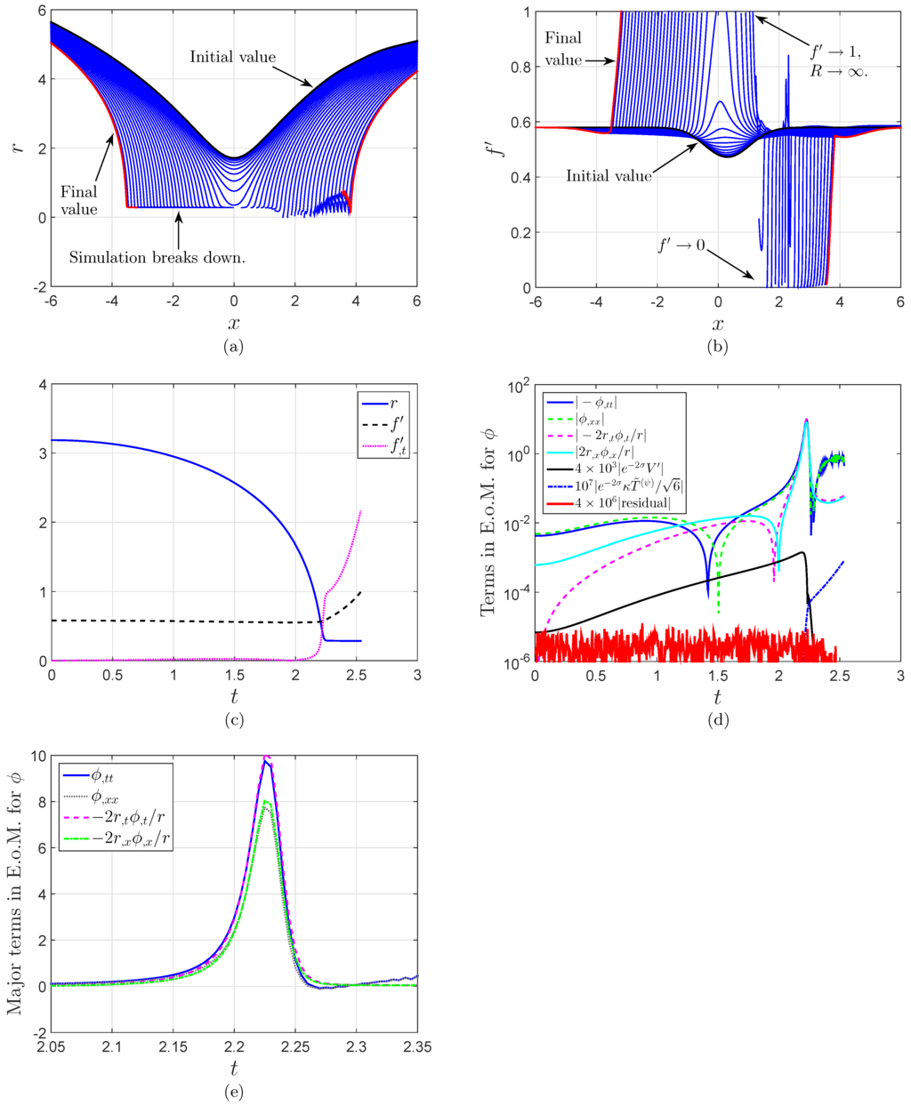
Figure 21.
(color online) A singularity problem in charge scattering for the Hu-Sawicki model Equation (30), . (a) and (b): evolutions of r and . The time interval between two consecutive slices is . (c) evolutions of r, , and on the the slice . (d) and (e): dynamical equation for ϕ on the slice . In (e), as the inner horizon is approached, . This equation describes a positive feedback, since is positive. As a result, when is positive, ϕ can be accelerated to zero rapidly. Correspondingly, goes to 1 as plotted in (b) and (c), and the Ricci scalar R becomes singular. Then the simulation breaks down as shown in (a).

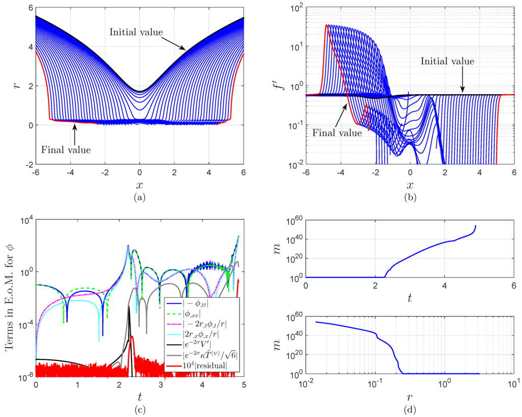
Figure 22.
(color online) Avoidance of the singularity problem in charge scattering for the combined model Equation (109), . (a) and (b): evolutions of r and . The time interval between two consecutive slices is . (c) dynamical equation for ϕ on the slice . (d) evolution of m on the slice .
Figure 22.
(color online) Avoidance of the singularity problem in charge scattering for the combined model Equation (109), . (a) and (b): evolutions of r and . The time interval between two consecutive slices is . (c) dynamical equation for ϕ on the slice . (d) evolution of m on the slice .

9. Summary
In this paper, we studied scalar collapses in flat, Schwarzschild, and Reissner-Nordström geometries in gravity numerically. Approximate analytic solutions for different types of collapses were partially obtained. One dark energy singularity problem was discussed. We summarize our work on computational and physical issues separately below.
9.1. Computational Issues
- (1)
- The Jordan frame vs the Einstein frame. The field equations for gravity in the Jordan frame are more complex than those in general relativity. Therefore, for ease of computation, we transform gravity from the Jordan frame into the Einstein frame, in which the formalism can be formally treated as Einstein gravity coupled to a scalar field.
- (2)
- vs. in double-null coordinates. In the studies of mass inflation, the format of the Kruskal-like coordinates, , is usually used. In the field equations, many terms are mixed derivatives of u and v, e.g., . In this paper, we used the format instead, , with and . In the line element, one coordinate is timelike, and the rest are spacelike. We are used to this setup. It is more convenient and more intuitive to use this set of coordinates. Moreover, for the choice, spatial and temporal derivatives are usually separated, e.g., .We set the initial conditions close to those in a Reissner-Nordström geometry. With this setup, it is convenient to test the code. Removing the terms related to the scalar fields, we can test our code by comparing the numerical results to the analytic ones in a Reissner-Nordström geometry. Moreover, by comparing numerical results for charge scattering to the dynamics in the Reissner-Nordström geometry, we can obtain intuitions as to how the scalar fields affect the geometry.
- (3)
- Cauchy horizon: infinite or local regions? As implied by Equation (28), the exact inner horizon is at the regions where and are infinite. However, r still can be very close to the inner horizon even when and take moderate values. Consequently, at regions where and take some moderate values, the scalar fields and the inner horizon still can have strong interactions, resulting in mass inflation.
9.2. Physical Issues
- (1)
- Scalar collapse in gravity vs scalar collapse in general relativity. In scalar collapse, the scalar degree of freedom plays a similar role as a physical scalar field in general relativity. Regarding the physical scalar field in the case, when is negative (positive), the physical scalar field is suppressed (magnified) by ϕ.
- (2)
- The inner horizon in a Reissner-Nordström black hole vs the central singularity in a Schwarzschild black hole. These two share some similarities.For Reissner-Nordström and Schwarzschild black holes, throughout the whole spacetime, the Misner-Sharp mass function is constant. When a scalar field impacts the inner horizon of a Reissner-Nordström black hole, the scalar field can modify the geometry in the vicinity of the inner horizon significantly, especially on . The inner horizon contracts and mass inflation takes place. In neutral scalar collapse toward a Schwarzschild black hole formation, the scalar field can also modify the geometry in the vicinity of the central singularity dramatically, especially on the metric component σ [20]. Then mass inflation also happens.The Belinskii, Khalatnikov, and Lifshitz (BKL) conjecture is an important result on dynamics in the vicinity of a spacelike singularity [76,77,78,79]. The first statement of this conjecture is that as the singularity is approached, the dynamical terms dominate the spatial terms in the field equations. In other words, the way gravity changes over time is more important than the variation of the gravitational field from one location to the next [79]. We would like to say that, to a large extent, later evolutions in a strong gravitational field largely erase away the initial information on the connections between neighboring points. As discussed in Reference [20] and also in this paper, in double-null coordinates, using the above argument, one can interpret the following behaviors displayed in numerical simulations: near the central singularity of a Schwarzschild black hole and also near the inner horizon of a Reissner-Nordström black hole, there areIn this paper, it was shown that Equation (110) can explain the causes of mass inflation, while Equation (111) can explain the dark energy singularity problem in collapse.The second and third statements of the BKL conjecture are that i) the metric terms will dominate the matter field terms, while the matter field may not be negligible if it is a scalar field; ii) the dynamics of the metric components and the matter fields is described by the Kasner solution. These two statements were confirmed in simulations of neutral scalar collapse in gravity in Reference [20] and in general relativity in Reference [41]. The second statement was also verified in charge scattering in this paper. However, the third statement on Kasner solution may not apply to the dynamics near the inner horizon in charge scattering.
- (3)
- Compact stars vs black holes in gravity. The internal structure of compact stars is usually in an equilibrium state and is static. In gravity, inside compact stars, the scalar degree of freedom, , can be coupled to the energy density of the stars and then is not very free to move. However, due to strong gravity, the internal structure of black holes is dynamical. and the matter fields are decoupled. As a result, is more free to move than in the compact stars case. It can keep increasing or decreasing until singularities are met.
- (4)
- Dark energy singularity problem: cosmology (or static compact objects) vs black hole physics. In dark energy gravity, the Ricci scalar R can be singular in both cosmology and black hole physics. We consider a homogeneous cosmological model. Using the flat Friedmann-Robertson-Walker metric,the equation of motion for iswhere H is the Hubble parameter. Due to the finiteness of the potential barrier, the force from a perturbation of may push to 1. Correspondingly, the Ricci scalar goes to singularity [72]. In the black hole case that we discussed in this paper, the equation of motion for has more complex structure Equation (36),As the central singularity of a Schwarzschild black hole or the inner horizon of a Reissner-Nordström black hole is approached, the above equation can be simplified as Equation (111), and gravity from the black hole, , can cause a similar singularity problem as in cosmology or static compact stars.
- (5)
- The combined model and the model: singular or non-singular? At the center of a Schwarzschild black hole and in the very early Universe, the tidal forces are singular, and general relativity fails. Taking into account quantum-gravitational effects, Starobinsky obtained an model, . This model has a non-singular de Sitter solution, which is unstable both to the past and to the future [42,43]. In Section 5, scalar collapse in a Schwarzschild geometry for the combined model (a combination of dark energy model and model) was explored. A new Schwarzschild black hole, including a new central singularity, can be formed. Moreover, under certain initial conditions, and R can be pushed to infinity as the central singularity is approached. In Reference [73], scalar collapse in flat geometry for the model was simulated. Similar results were obtained. Namely, the classical singularity problem, which is present in general relativity, remains in collapse in these models.
- (6)
- Inside vs. outside black holes: local vs global. Throughout the whole spacetime of stationary Schwarzschild and Reissner-Nordström black holes, the Misner-Sharp mass function is equal to the black hole mass. For a gravitational collapsing system, at asymptotic flat regions, the mass function describes the total mass of the dynamical system. However, in this system, near the central singularity of a Schwarzschild black hole or near the inner horizon of a Reissner-Nordström black hole, the dynamics is local. Then the mass function does not provide global information on the mass of the collapsing system.
In summary, in this paper, we studied scalar collapses in flat, Schwarzschild, and Reissner-Nordström geometries in gravity. For convenience and intuitiveness, in simulating scalar collapses in Schwarzschild and Reissner-Nordström geometries, Kruskal and Kruskal-like coordinates were used, respectively. Approximate analytic solutions for different types of collapses were partially obtained. Causes and avoidance of a dark energy singularity problem in collapse were discussed.
Acknowledgments
The authors would like to thank Andrei V. Frolov, José T. Gálvez Ghersi, Ken-ichi Nakao, and Dong-han Yeom for useful discussions. The authors also thank the referees for the helpful comments.
Author Contributions
All authors have contributed to this paper. All authors have read and approved the final version.
Conflicts of Interest
The authors declare on conflict of interest.
A. Equations of Motion for a Physical Scalar Field and in the Einstein Frame
In this appendix, based on the equations of motion for a massless physical scalar field ψ and the scalar degree of freedom in the Jordan frame for gravity, we derive the corresponding equations in the Einstein frame. In the transformation from the Jordan frame into the Einstein frame, we use and , where a tilde denotes that the quantity is in the Einstein frame.
For a scalar field ψ, the first covariant derivatives of ψ are equal in two frames, since they are both equal to the partial derivative [80]:
Then for the first contravariant derivative of ψ, there is
For , we have [81]
In the Jordan frame, for a massless scalar field ψ, there is
Combining Equations (117) and (118) yields the equation of motion for ψ in the Einstein frame Equation (22).
In the special case of , there is
Combining Equations (9), (10), (17), (24), and (119) gives the equation of motion for ϕ in the Einstein frame Equation (21).
B. Reissner-Nordström Metric in Kruskal-Like Coordinates
The Reissner-Nordström metric in Kruskal-like coordinates was obtained in Reference [52] (also see Reference [53]). For reference concern, we list the derivations here via analog to the Schwarzschild black hole case in the form of Reference [53].
We start from the Reissner-Nordström metric in the conventional form,
where
Considering the radial null curves along which , we have
The solution to the above equation can be expressed as
where
B.1. Patch I:
(i) of Patch I
As implied in Equation (125), the inner and outer horizons in the metric Equation (128) are pushed to infinity. To compact them into finite space, we define
Rewrite Equation (125) as
Using Equations (121), (127), (129), and (130), the line element Equation (128) can be converted into the following format
Note that we get used to coordinate systems in which one coordinate is timelike and the rest are spacelike. So defining
one can rewrite the metric Equation (131) as
Moreover, using Equations (125), (132), and (133), r and t can be expressed as
(ii) of Patch I
Define
Similar to the case of , one can obtain
B.2. Patch II:
(i) of Patch II
Define
In a similar routine as in Patch I, the metric for the spacetime of can be obtained as
with
(ii) of Patch II
Define
Then we have
C. Einstein Tensor and Energy-Momentum Tensor for a Massive Scalar Field
In this appendix, we give specific expressions for the Einstein tensor and the energy-momentum tensor for a massive scalar field. In double-null coordinates expressed by Equations (25) and (26), some components of the Einstein tensor can be expressed as follows:
For a massive scalar field with an energy-momentum tensor
there are
The equations obtained in this appendix can be used to derive the field equations discussed in Section 3.1.
References
- Burko, L.M.; Ori, A. (Eds.) Internal Structure of Black Holes and Spacetime Singularities; Institute of Physics Publishing: Bristol, UK, 1998.
- Brady, P.R. The Internal Structure of Black holes. Prog. Theor. Phys. Suppl. 1999, 136, 29–44. [Google Scholar] [CrossRef]
- Berger, B.K. Numerical Approaches to Spacetime Singularities. Living Rev. Relativ. 2002, 5, 1. [Google Scholar] [CrossRef]
- Joshi, P.S. Gravitational Collapse and Spacetime Singularities; Cambridge University Press: Cambridge, UK, 2007. [Google Scholar]
- Henneaux, M.; Persson, D.; Spindel, P. Spacelike Singularities and Hidden Symmetries of Gravity. Living Rev. Relativ. 2008, 11, 1. [Google Scholar] [CrossRef]
- Price, R.H. Nonspherical Perturbations of Relativistic Gravitational Collapse. I. Scalar and Gravitational Perturbations. Phys. Rev. D 1972, 5, 2419–2438. [Google Scholar] [CrossRef]
- Clifton, T.; Ferreira, P.G.; Padilla, A.; Skordis, C. Modified gravity and cosmology. Phys. Rep. 2012, 513, 1–189. [Google Scholar] [CrossRef]
- Sotiriou, T.P.; Faraoni, V. f(R) Theories Of Gravity. Rev. Mod. Phys. 2010, 82, 451–497. [Google Scholar] [CrossRef]
- Felice, A.D.; Tsujikawa, S. f(R) Theories. Living Rev. Relativ. 2010. [Google Scholar] [CrossRef]
- Nojiri, S.; Odintsov, S. D. Unified cosmic history in modified gravity: From F(R) theory to Lorentz non-invariant models. Phys. Rept. 2011, 505, 59–144. [Google Scholar] [CrossRef]
- Capozziello, S.; de Laurentis, M. Extended Theories of Gravity. Phys. Rept. 2011, 509, 167–321. [Google Scholar] [CrossRef]
- Cruz-Dombriz, A.; de la Dobado, A.; Maroto, A.L. Black Holes in f(R) theories. Phys. Rev. D 2009, 80, 124011. [Google Scholar] [CrossRef]
- Olmo, G.J.; Rubiera-Garcia, D. Palatini f(R) Black Holes in Nonlinear Electrodynamics. Phys. Rev. D 2011, 84, 124059. [Google Scholar] [CrossRef]
- Nojiri, S.; Odintsov, S.D. Anti-Evaporation of Schwarzschild-de Sitter Black Holes in F(R) gravity. Class. Quantum Gravity 2013, 30, 125003. [Google Scholar] [CrossRef]
- Sebastiani, L.; Momeni, D.; Myrzakulov, R.; Odintsov, S.D. The instabilities and (anti)-evaporation of Schwarzschild-de Sitter black holes in modified gravity. Phys. Rev. D 2013, 88, 104022. [Google Scholar] [CrossRef]
- Nojiri, S.; Odintsov, S.D. Instabilities and Anti-Evaporation of Reissner-Nordström Black Holes in modified F(R) gravity. Phys. Lett. B 2014, 735, 376–382. [Google Scholar] [CrossRef]
- Avelino, P.P.; Hamilton, A.J.S.; Herdeiro, C.A.R. Mass Inflation in Brans-Dicke gravity. Phys. Rev. D 2009, 79, 124045. [Google Scholar] [CrossRef]
- Borkowska, A.; Rogatko, M.; Moderski, R. Collapse of Charged Scalar Field in Dilaton Gravity. Phys. Rev. D 2011, 83, 084007. [Google Scholar] [CrossRef]
- Hwang, D.-I.; Lee, B.-H.; Yeom, D.-H. Mass inflation in f(R) gravity: A conjecture on the resolution of the mass inflation singularity. J. Cosmol. Astropart. Phys. 2011, 2011, 006. [Google Scholar] [CrossRef]
- Guo, J.-Q.; Wang, D.; Frolov, A.V. Spherical collapse in f(R) gravity and the Belinskii-Khalatnikov-Lifshitz conjecture. Phys. Rev. D 2014, 90, 024017. [Google Scholar] [CrossRef]
- Simpson, M.; Penrose, R. Internal instability in a Reissner-Nordström black hole. Int. J. Theor. Phys. 1973, 7, 183–197. [Google Scholar] [CrossRef]
- Dafermos, M. Stability and instability of the Cauchy horizon for the spherically symmetric Einstein-Maxwell-scalar field equations. Ann. Math. (N. Y.) 2003, 158, 875–928. [Google Scholar] [CrossRef]
- Dafermos, M. Black holes without spacelike singularities. Commun. Math. Phys. 2014, 332, 729–757. [Google Scholar] [CrossRef]
- Ringström, H. Origins and development of the Cauchy problem in general relativity. Class. Quantum Gravity 2015, 32, 124003. [Google Scholar] [CrossRef]
- Isenberg, J. On Strong Cosmic Censorship. 2015; arXiv:1505.06390[gr-qc]. [Google Scholar]
- Poisson, E.; Israel, W. Inner-horizon instability and mass inflation in black holes. Phys. Rev. Lett. 1989, 63, 1663–1666. [Google Scholar] [CrossRef] [PubMed]
- Poisson, E.; Israel, W. Internal structure of black holes. Phys. Rev. D 1990, 41, 1796–1809. [Google Scholar] [CrossRef]
- Barrabes, C.; Israel, W.; Poisson, E. Collision of light-like shells and mass inflation in rotating black holes. Class. Quantum Gravity 1990, 7, L273–L278. [Google Scholar] [CrossRef]
- Gnedin, N.Y.; Gnedina, M.L. Instability of the internal structure of a Reissner-Nordström black hole. Sov. Astron. 1992, 36, 296, (Astron. Zh. 1992, 69, 584–592.). [Google Scholar]
- Gnedin, M.L.; Gnedin, N.Y. Destruction of the Cauchy horizon in the Reissner-Nordstrom black hole. Class. Quantum Gravity 1993, 10, 1083–1102. [Google Scholar] [CrossRef]
- Brady, P.R.; Smith, J. Black hole singularities: A numerical approach. Phys. Rev. Lett. 1995, 75, 1256–1259. [Google Scholar] [CrossRef] [PubMed]
- Burko, L.M. Structure of the black hole’s Cauchy horizon singularity. Phys. Rev. Lett. 1997, 79, 4958–4961. [Google Scholar] [CrossRef]
- Burko, L.M.; Ori, A. Late-time evolution of nonlinear gravitational collapse. Phys. Rev. D 1997, 56, 7820–7832. [Google Scholar] [CrossRef]
- Hansen, J.; Khokhlov, A.; Novikov, I. Physics of the interior of a spherical, charged black hole with a scalar field. Phys. Rev. D 2005, 71, 064013. [Google Scholar] [CrossRef]
- Hod, S.; Piran, T. Mass Inflation in Dynamical Gravitational Collapse of a Charged Scalar Field. Phys. Rev. Lett. 1998, 81, 1554–1557. [Google Scholar] [CrossRef]
- Oren, Y.; Piran, T. Collapse of charged scalar fields. Phys. Rev. D 2003, 68, 044013. [Google Scholar] [CrossRef]
- Burko, L.M.; Ori, A. Analytic study of the null singularity inside spherical charged black holes. Phys. Rev. D 1998, 57, R7084–R7088. [Google Scholar] [CrossRef]
- Burko, L.M. Strength of the null singularity inside black holes. Phys. Rev. D 1999, 60, 104033. [Google Scholar] [CrossRef]
- Hu, W.; Sawicki, I. Models of f(R) Cosmic Acceleration that Evade Solar-System Tests. Phys. Rev. D 2007, 76, 064004. [Google Scholar] [CrossRef]
- Cai, R.G.; Cao, L.M.; Hu, Y.P.; Ohta, N. Generalized Misner-Sharp Energy in f(R) Gravity. Phys. Rev. D 2009, 80, 104016. [Google Scholar] [CrossRef]
- Guo, J.-Q.; Joshi, P.S. Interior dynamics of neutral and charged black holes. 2015; arXiv:1507.01806[gr-qc]. [Google Scholar]
- Starobinsky, A.A. A new type of isotropic cosmological models without singularity. Phys. Lett. B 1980, 91, 99–102. [Google Scholar] [CrossRef]
- Vilenkin, A. Classical and quantum cosmology of the Starobinsky inflationary model. Phys. Rev. D 1985, 32, 2511–2521. [Google Scholar] [CrossRef]
- Nojiri, S.; Odintsov, S.D. The future evolution and finite-time singularities in F(R)-gravity unifying the inflation and cosmic acceleration. Phys. Rev. D 2008, 78, 046006. [Google Scholar] [CrossRef]
- Bamba, K.; Nojiri, S.; Odintsov, S.D. Future of the universe in modified gravitational theories: Approaching to the finite-time future singularity. J. Cosmol. Astropart. Phys. 2008, 10, 045. [Google Scholar] [CrossRef]
- Capozziello, S.; de Laurentis, M.; Nojiri, S.; Odintsov, S.D. Classifying and avoiding singularities in the alternative gravity dark energy models. Phys. Rev. D 2009, 79, 124007. [Google Scholar] [CrossRef]
- Appleby, S.A.; Battye, R.A.; Starobinsky, A.A. Curing singularities in cosmological evolution of F(R) gravity. J. Cosmol. Astropart. Phys. 2010, 06, 005. [Google Scholar] [CrossRef]
- Elizalde, E.; Nojiri, S.; Odintsov, S.D.; Sebastiani, L.; Zerbini, S. Non-singular exponential gravity: A simple theory for early- and late-time accelerated expansion. Phys. Rev. D 2011, 83, 086006. [Google Scholar] [CrossRef]
- Bamba, K.; Nojiri, S.; Odintsov, S.D. Time-dependent matter instability and star singularity in F(R) gravity. Phys. Lett. B 2011, 698, 451–456. [Google Scholar] [CrossRef]
- Poisson, E. A Relativist’s Toolkit: The Mathematics of Black-Hole Mechanics; Cambridge University Press: Cambridge, UK, 2004. [Google Scholar]
- Frolov, A.V. Is It Really Naked? On Cosmic Censorship in String Theory. Phys. Rev. D 2004, 70, 104023. [Google Scholar] [CrossRef]
- Graves, J.C.; Brill, D.R. Oscillatory Character of Reissner-Nordström Metric for an Ideal Charged Wormhole. Phys. Rev. 1960, 120, 1507–1513. [Google Scholar] [CrossRef]
- Reall, H. Lecture Notes on Black Holes. Available online: http://www.damtp.cam.ac.uk/user/hsr1000/black_holes_lectures_2015.pdf (accessed on 29 August 2015).
- Nunez, A.; Solganik, S. The content of f(R) gravity. 2004; arXiv:hep-th/0403159. [Google Scholar]
- Dolgov, A.D.; Kawasaki, M. Can modified gravity explain accelerated cosmic expansion? Phys. Lett. B 2003, 573, 1–4. [Google Scholar] [CrossRef]
- Amendola, L.; Gannouji, R.; Polarski, D.; Tsujikawa, S. Conditions for the cosmological viability of f(R) dark energy models. Phys. Rev. D 2007, 75, 083504. [Google Scholar] [CrossRef]
- Guo, J.-Q.; Frolov, A.V. Cosmological dynamics in f(R) gravity. Phys. Rev. D 2013, 88, 124036. [Google Scholar] [CrossRef]
- Khoury, J.; Weltman, A. Chameleon Fields: Awaiting Surprises for Tests of Gravity in Space. Phys. Rev. Lett. 2004, 93, 171104. [Google Scholar] [CrossRef] [PubMed]
- Khoury, J.; Weltman, A. Chameleon Cosmology. Phys. Rev. D 2004, 69, 044026. [Google Scholar] [CrossRef]
- Chiba, T.; Smith, T.L.; Erickcek, A.L. Solar System constraints to general f(R) gravity. Phys. Rev. D 2007, 75, 124014. [Google Scholar] [CrossRef]
- Tamaki, T.; Tsujikawa, S. Revisiting chameleon gravity - thin-shells and no-shells with appropriate boundary conditions. Phys. Rev. D 2008, 78, 084028. [Google Scholar] [CrossRef]
- Tsujikawa, S.; Tamaki, T.; Tavakol, R. Chameleon scalar fields in relativistic gravitational backgrounds. J. Cosmol. Astropart. Phys. 2009, 05, 020. [Google Scholar] [CrossRef]
- Guo, J.-Q. Solar system tests of f(R) gravity. Int. J. Mod. Phys. D 2014, 23, 1450036. [Google Scholar] [CrossRef]
- Pretorius, F. Numerical Relativity Using a Generalized Harmonic Decomposition. Class. Quantum Gravity 2005, 22, 425–452. [Google Scholar] [CrossRef]
- Sorkin, E.; Piran, T. Effects of Pair Creation on Charged Gravitational Collapse. Phys. Rev. D 2001, 63, 084006. [Google Scholar] [CrossRef]
- Golod, S.; Piran, T. Choptuik’s Critical Phenomenon in Einstein-Gauss-Bonnet Gravity. Phys. Rev. D 2012, 85, 104015. [Google Scholar] [CrossRef]
- Misner, C.W.; Sharp, D.H. Relativistic Equations for Adiabatic, Spherically Symmetric Gravitational Collapse. Phys. Rev. 1964, 136, B571–B576. [Google Scholar] [CrossRef]
- Hayward, S.A. Gravitational energy in spherical symmetry. Phys. Rev. D 1996, 53, 1938–1949. [Google Scholar] [CrossRef]
- Baumgarte, T.W.; Shapiro, S.L. Numerical Relativity: Solving Einstein’s Equations on the Computer; Cambridge University Press: Cambridge, UK, 2010. [Google Scholar]
- Csizmadia, P.; Racz, I. Gravitational collapse and topology change in spherically symmetric dynamical systems. Class. Quantum Gravity 2010, 27, 015001. [Google Scholar] [CrossRef]
- Garfinkle, D. Choptuik scaling in null coordinates. Phys. Rev. D 1995, 51, 5558–5561. [Google Scholar] [CrossRef]
- Frolov, A.V. A Singularity Problem with f(R) Dark Energy. Phys. Rev. Lett. 2008, 101, 061103. [Google Scholar] [CrossRef] [PubMed]
- Guo, J.-Q.; Joshi, P.S. Spherical collapse for the Starobinsky R2 model. 2015; in preparation. [Google Scholar]
- Hong, S.E.; Hwang, D.-I.; Stewart, E.D.; Yeom, D.-H. The causal structure of dynamical charged black holes. Class. Quantum Gravity 2010, 27, 045014. [Google Scholar] [CrossRef]
- Kawai, H.; Yokokura, Y. Phenomenological Description of the Interior of the Schwarzschild Black Hole. Int. J. Mod. Phys. A 2015, 30, 1550091. [Google Scholar] [CrossRef]
- Belinskii, V.A.; Kalathnikov, I.M.; Lifshitz, E.M. Oscillatory Approach to a Singular Point in the Relativistic Cosmology. Adv. Phys. 1970, 19, 525–573. [Google Scholar] [CrossRef]
- Belinskii, V.A.; Khalatnikov, I.M. Effect of scalar and vector fields on the nature of the cosmological singularity. Zh. Eksp. Teor. Fiz. 1972, 63, 1121–1134. [Google Scholar]
- Belinskii, V.A. On the cosmological singularity. Int. J. Mod. Phys. D 2014, 23, 1430016. [Google Scholar] [CrossRef]
- BKL conjecture. Available online: http://www.einstein-online.info/dictionary/bkl-conjecture (accessed on 29 August 2015).
- Carroll, S. Spacetime and Geometry: An Introduction to General Relativity; Addison-Wesley: San Francisco, U.S.A., 2003. [Google Scholar]
- Landau, L.D.; Lifshitz, E.M. The Classical Theory of Fields; Pergamon Press: Oxford, UK, 1971; Volume 2. [Google Scholar]
© 2015 by the authors; licensee MDPI, Basel, Switzerland. This article is an open access article distributed under the terms and conditions of the Creative Commons Attribution license (http://creativecommons.org/licenses/by/4.0/).