Abstract
This article aims to resolve a particular production planning and workforce assignment problem. Many production lines may have different production capacities while producing the same product. Each production line is composed of three production stages, and each stage requires different periods of times and numbers of workers. Moreover, the workers will have different skill levels which can affect the number of workers required for production line. The number of workers required in each farm also depends on the amount of pigs that it is producing. Production planning must fulfill all the demands and can only make use of the workers available. A production plan aims to generate maximal profit for the company. A mathematical model has been developed to solve the proposed problem, when the size of problem increases, the model is unable to resolve large issues within a reasonable timeframe. A metaheuristic method called adaptive large-scale neighborhood search (ALNS) has been developed to solve the case study. Eight destroy and four repair operators (including ant colony optimization based destroy and repair methods) have been presented. Moreover, three formulas which are used to make decisions for acceptance of the newly generated solution have been proposed. The present study tested 16 data sets, including the case study. From the computational results of the small size of test instances, ALNS should be able to find optimal solutions for all the random data sets in much less computational time compared to commercial optimization software. For medium and larger test instance sizes, the findings of the heuristics were 0.48% to 0.92% away from the upper bound and generated within 480–620 h, in comparison to the 1 h required for the proposed method. The Ant Colony Optimization-based destroy and repair method found solutions that were 0.98 to 1.03% better than the original ALNS.
1. Introduction
Open innovation is a hot issue for firms that wish to stay up to date. Firm operating in an environment of open innovation will have better chances to track the changing of new world social movements. Product producing companies must always maintain their technological planning and develop new methods so that they can adjust their operations to minimize costs as far as possible. Good planning serves to reduce costs and increase profits for the firm, especially in the Thai agricultural industry. Thai agricultural firms are often not interested in highly productive technologies and effective planning methods, which reduces their profitability.
Agricultural products are one of Thailand’s main exports, particularly in terms of meat exports. Thailand annually (2018) produces 14.54 million tons of pig meat, a 7.2% increase from last year. The average annual growth rate of pig production is currently 3.2%, and is therefore very high. Increasing pig production in Thailand is due to higher sales prices motivating farmers to expand their farms or establish new farms, thereby dramatically increasing pig production. Buriram province has a large number of pig farms because of the favorable climate and the basic farming knowledge that is passed between family generations.
Research Motivation: Pornprasert Farm Co., Ltd. has been operating pig farms for more than 40 years. It is considered a large company and produces more than 1000 pigs monthly and it has 37 pig farms, each with different capacities. Pig production is divided into three stages: new born (ages 0 to 2 weeks); growing stage (ages 2 to 6 weeks); and mature (ages 6 to 8 weeks). The three pig production stages require different numbers of workers to care of them. There are a limited number of workers able to work on the farms, and each worker has a different level of experience. More experienced workers can be used to compensate a few unexperienced workers, but experienced workers demand higher daily wages. Decisions must be made regarding the design and size of each farm to be opened, and which workers have to be assigned to each farm to satisfy customer demands. Planning must consider the maximum profit that can be generated, product prices, and labor costs.
Contribution of the article: Srivarapongse and Pijitbanjong (2019) [1] presents a differential evolution algorithm to discover the solution of the special case of the assignment problem. The driver of the harvester has been assigned to the sugarcane harvest set. Then the harvest set has been assigned to the sugarcane field whereas the daily maximum profit is generated. Worker skills and experiences and machine capacity and type are considered in our algorithm. In the present article, the pig production stages (which require different numbers of workers) is added and the farms’ mature pig production schedules have also been added, while multiple periods have been considered. Moreover, the limited number of workers in each period is presented and the research considers how highly skilled workers may compensate unexperienced worker, something which is mentioned in previous study.
With regards to the proposed method, ant colony optimization (ACO) is combined with Adaptive Large Neighborhood Search (ALNS) to improve the effectiveness of the original ALSN. Finally, three new formulas, which are used to accept or reject the newly generated solution, have been proposed and presented.
2. Literature Review
This research is concerned with production planning where the farming production schedule has been decided and the worker assignments to assign the workers to work in the farms has been determined.
The problem can be divided into two groups: (1) assign workers to begin production of some amount of pigs in a particular period so that the farm will have enough pigs to supply customer demands; and (2) for each period, the available workers will be assigned to the operating farms. Determining what period each farm should begin production affects the number of pigs that can be produced in each period as well as the required number of workers and amount of resources. All of these factors affect the company’s costs and profits. The literature review has focused on two closely related keywords: assignment problem, and generalized assignment problem.
The worker assignment problem has been intensively studied. Al-Yakoob et al. [2] propose the teaching assistant assignment to school courses method. A weekly planning method for the teaching of some courses has been determined in order to minimize the working hours of the teaching assistant. This type of problem is sometimes called the ‘timetabling problem’ which is proven as the non-polynomial hard problem (NP-hard problem) [3,4,5].
In the present study, the workers have different skills levels and costs. Therefore, assigning different workers to different farms and periods will generate costs differences. Moreover, the workers must be constantly circulated due to the changing worker requirements for each production stage, further compounding the problems beyond timetabling issues. The next section of the literature review will focus on the assignment problem (AP).
There are variances to the assignment problem, such as quadratic assignment problems and generalized assignment problems. Srivarapongse and Pijitbanjong [1] recently proposed a methodology to resolve the generalized assignment problems (GAP). In that study, the proposed methodology was applied to the sugarcane harvesting system, and considered driver skill and experience, and the machine types and capacities.
The generalized assignment problem (GAP) is an extension version of the assignment problem in which multiple tasks are able to be assigned to one agent. The different assignments may consume a different volume of resources. Ross and Soland [6] first proposed GAP and proved that it was an NP-hard problem [7]. After that, it was proved to be NP-complete by Chu and Beasley et al. [8]. The exact methods are presented and tested with a generated data set that has no additional constraints.
GAP has been widely studied by many researchers who try to solve real-world applications, such as Osorio and Laguna [9], who solve the GAP where worker availability and job rotation is considered. The days worked are also considered by Alfares [10] and Elshafei [11]. Other extension of the GAP is to consider more than one assignment, this is called a multi-level GAP. Recently, finding the location and allocation of tasks have been considered while solving GAP [12].
From the review of the problem and the methodology, the proposed problem refers to a combination between assignment and scheduling problems. These problems aim to maximize profit generated from pig production for the whole planning horizon, as limited by the workers and customer demands. A new class of problem is therefore proposed in the present article.
The problem has the following attributes: (1) lead time is required in one assignment, therefore when the assignment has been done in certain period, it needs to keep the server free for some time; (2) during the production time, the resources required can change to serve the different stages of pig production; and (3) the assignment in the current period is used to serve demand in later periods due to the production time and each assignment generating different production rates according to farm capacities. The proposed problem combines the assignment and scheduling problems which is an NP-hard problem, as explained above.
A heuristics approach is therefore required to solve the problem. Well-known metaheuristics such as the variable neighborhood search [13,14], ant colony optimization [15], differential evolution algorithm (DE) [16,17] genetic algorithm (GA) [18], and the adaptive large neighborhood search [19].
The ant colony optimization (ACO) has been used in many research areas such as vehicle routing problem [20] and network problems [21,22]. ACO is a nature inspired heuristic, inspired by the ant behavior when searching for food. It is comprised of two main steps which are (1) construction of the initial solution using heuristics information; (2) update of the heuristic information. There are many ways to improve the efficiency of the ant colony optimization. The most effective choice that has often been used is the addition of strong local searches for the performance increase of the ACO [23]. An excellent review of the ACO was proposed by Blum et al. (2011) [24]. The ACO is one of the stochastic search heuristics. One of the most powerful stochastic searches found in the literature is the adaptive large neighborhood search (ALNS). This method will be used in our research since it is a fast and effective algorithm which is widely used to solve many combinatorial optimizations. Ropke and Pisinger [25] first proposed ALNS, which has four general steps: (1) construct the initial result; (2) pick the randomly selected destroy operator; (3) choose the randomly selected repair operator; and (4) accept or reject the new solution and the renew heuristic information. Steps (2) to (4) are then executed again once the heuristic’s information is updated [26].
Various researchers have applied the ALNS in many research areas, for example in the resource-constrained project scheduling problem [27], the selective and periodic inventory routing problem [14], and the rural postman problem with time windows [28].
ALNS not only has been used individually, with some researchers having used it as a tool to improve the efficiency of other heuristics, such as using ALNS in the shaking phase of the variable neighborhood search (VNS) [29,30] and as the diversification strategy of VNS [31]. Besides, ALNS is incorporated with other heuristics and is also used as a hybrid with the well-known methods such as the Tabu Search [32] and greedy randomized adaptive search procedure (GRASP) [33], which have been applied successfully to solve the order batching problem and the pickup and delivery problems with transshipment, respectively.
From the methodologies review on the solution approaches to solve the proposed problem, ALNS will be used in connection with the ant colony optimization. The ant colony optimization is used in the present study in combination with ALNS due to many researchers having proved that the ACO is good for path planning problems, scheduling problems, and assignment problems [34,35,36,37,38,39,40,41,42,43]. In the present study, the destroy and repair methods were used to determine and select a sequence of the farms which were assigned for pig production. Therefore, the ACO was applied in the destroy and repair operators for the ALNS efficiency improvement.
There are some articles in the literature about pig production farms. Nadal-Roig and Plà (2014) [44] present linear programming (LP) that was used to solve the multisite systems and to transfer the pigs from different stages (new born, growing and mature stage). In this research, the pigs in different stages need to feed in different farms. The objective in this research is to maximize the total gross margin, which was calculated from the income of sales of mature pigs and the production costs, which included feeding, veterinary expenses and transportation costs. This research did not include the worker detail such as the number of workers required, level of experience, and cost of labor, therefore in our proposed method these attributes have been added. Later on, Nadal-Roig [45] extended the previous work by formulating the mathematical model for the whole Pig Supply Chain (PSC). The new trend in research with regard to pig production is to improve the efficiency of the PSC by integrating the production and distribution process in order get the optimal production and distribution planning [46,47], and to improve the transferring method from farm to farm to reduce the transferring cost and effectiveness [48,49]. The techniques that have been widely used in pig production planning are linear programming (LP), dynamics programming (DP) and hierarchic Markov models (HMM), because these methods can add different constraints to the main model therefore the LP can adapt to the real world problem [50,51,52,53,54]. In our proposed model, the efficiency and experience level of the pigs have been added into the model in which other models previously proposed have not yet mentioned. Because pig production is a hard problem, the techniques that have been proposed can solve the problems that are small. The problem that has a great number of farms or workers it is not possible to solve to optimality using these exact methods. Therefore, we have developed adaptive large neighborhood search (ALNS) to solve the large size of test instances.
3. Definitions of the Problem and Mathematical Construction
3.1. Problem Definitions
From Figure 1, the demand for pigs in Periods 5, 6 and 7 is 400, 400, and 200 pigs, respectively. The pig farms’ capacities are as follows A (400), B (200), C (250), D (500), and E (300). The production lead time of the pigs is four periods (month). Therefore, to meet demand in period 5, production must be started in period 1. Farms B and D will be assigned to produce 200 and 200 pigs. The new born pigs are assigned to be grown in Farms B and D, and they will remain new born pigs for two periods. One worker is required to care for 100 new born pigs. Workers with an experience level of 0.6, 0.5, 1.7, and 1.5 have been selected to work in the first period. Farm B produces 200 pigs, and therefore workers 1 (0.6) and 3 (0.5) who have a total sum experience equal to 2.3 were selected, while workers 2 and 4 were selected to take care of farm D which has a demand of 200 (two workers are needed and the sum of workers’ experience is 2.0). Each pig production stage requires different numbers of workers, with 100 new born pigs requiring one worker, the growing stage needs 0.8 workers per 100 pigs, and the maturity stage needs 0.5 workers per 100 pigs. The duration of each stage of pig production is also different.
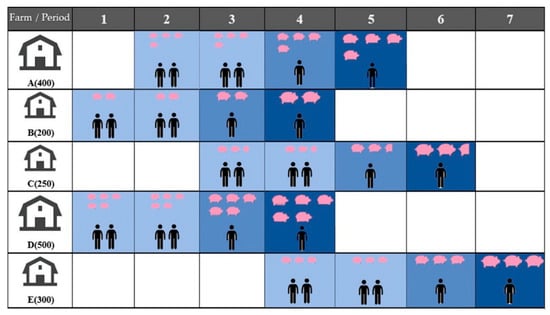
Figure 1.
Pig production plan.
3.2. Mathematical Construction
This section presents the mathematical model formulation used to compute the assignment problems in our case study.
Index
| i | illustrates the number of pig farms i = 1, 2, …, I |
| t | illustrates the time taken to feed pigs t = 1, 2, …, T |
| k | illustrates the workers which is used k = 1, 2, …, K |
Parameters
| Pi | The income from matured pigs of farm i (baht/pigs) |
| C | Cost of producing mature pigs (baht/pig) |
| Fi | Fixed cost of farm i (baht) |
| Number of new born pigs that can feed on the farm i | |
| Worker experience level k | |
| Daily worker wages k | |
| M | big-M coefficient |
| Dt | Demand for pigs in period t |
| L | Lead time to produce pigs |
| Duration of pigs in new born stage | |
| Duration of pigs in growing stage | |
| Duration of pigs in mature stage | |
| Minimum workers required for pigs in new born stage | |
| Minimum workers required for pigs in growing stage | |
| Minimum workers required for pigs in mature stage | |
| Size of farm i |
Decision Variables
| Yit | |
| Xit | |
| Oi | |
| Nkit | |
Objective function
Constraints
when
when to
when to
Objective function Z, which is shown in Formula (1), is purposed to obtain the highest profit, calculated by subtracting the profit generated by selling the mature pigs from the fixed opening cost of the farms and the labor costs. Constraint (2) determines that the farm can be opened at most one time during the planning horizon. Constraint (3) controls the number of pigs that can be produced only when the farms are in use. Constraint (4) shows that the farm cannot produce more pigs than its capacity. Constraint (5) determines that the total number of pigs produced by all the farms must fill the end-customer demands. Constraints (6) to (8) represent the controlled decision variable of all pig production stages. Constraints (9) to (11) requires that there must be enough workers to care for the pigs in all stages. Finally, Constraint (12) requires that each worker is assigned to at most one farm for each period.
The mathematical model shown above is coded in optimization software, and lingo v.11 has been used in our research. An example of the solution that was generated by Lingo v.11 is shown in Table 1.

Table 1.
Solution of the mathematical model generated by Lingo v.11.
An example of the number shown in Table 1, such as 3 (200), means at that period the farm has to produce 200 pigs and it needs three workers. When a farm starts to produce 200 at the new born stage it needs to execute other two stages which are the growing and mature stages. The new born, growing, and mature stages need three, two and one periods respectively. The number of periods in each stage is controlled by Formula (6)–(8). For each period needs to produce enough number of pigs to supply the demand at period t+L. From Table 1, farm B and D has to produce 200 and 200 pigs, respectively, due to the amount needed to fulfill the demand of Period 5. This requirement is controlled by Formula (5). In our planning, a particular farm can start the production only one time during the planning horizon and it is controlled by Formula (2) while the amount of production is controlled by Formulas (3) and (4), which should not exceed its capacity (Formula (3)). The number of workers used in each period is calculated from the new born stage. In this example, experiences of workers are assumed to be equal to the value of 1.00. Three, two and one workers are needed for 200 new born pigs, and the growing and mature stages of pig production.
4. The Proposed Methods
As addressed above, ALNS comprises four steps: (1) creating the initial solution; (2) choosing the destroy operator and performing the destroy operator; (3) picking the repair operator and performing the repair operator; and (4) renewing the parameters and the current solution. Steps (2) to (4) are iteratively simulated until the maximum number of iterations have been reached, upon which the algorithm is then ended. The ALNS steps will now be further explained.
4.1. Construct Initial Solution
The first solution is created from a string of real values.
Step 1: Generate two random vectors. The first vector has a dimension of 1*N where N is the number of farms and the second vector has a dimension of 1*W where W is the number of workers.
Step 2: Sort each vector according to the value in each vector position.
Step 3: For each period, assign the farms step-by-step (using vector 1) to operate according to the order given in Step 2. The assignment of the farm to be operated is determined from the demand of period t + L where t is current period and L is the lead time to produce mature pigs.
Step 4: Continue assigning farms to produce mature pigs until all customer demand has been satisfied.
Step 5: For each period, assign workers to the operated farm according to the order of workers in vector 2 and the number of workers required in each period based on the pig stages in that period.
Table 2 shows the random vector before and after being sorted. The value in the vector position is randomly generated. Table 3 shows the vector shown in Table 2 after being sorted. If customer demand in Periods 4 to 6 is 1000, 750, and 750, respectively, the capacity of Farms 1 to 8 will be 400, 500, 500, 400, 600, 620, 550, and 450, respectively. Each period has 12 workers to work. Each worker has daily wages of 300, 350, 500, 400, 450, 450, 400, 300, 450, 450, 500, and 350 baht, respectively. The daily wages are based on worker experience, which are 1.0, 1.3, 1.4, 1.4, 1.4, 1.35, 1.2, 1.45, 1.25, 1.45, 1.3, and 1.35, respectively. If Stages 1, 2, and 3 of pig production have two, one, and one workers required per 500 pigs, respectively and if a certain farm has 1000 new born pigs, it will need four workers for the first stage. If Workers 2, 3, and 4 are selected to work, it is sufficient due to their combined experience of 1.3, 1.4, and 1.4 (total 4.1). The production lead time of the pigs is divided into three periods. The new born pig stage lasts two periods, while the growing and mature stages last for one period each. Therefore, the results of using vectors #1 and #2 to schedule the farm and assign workers are shown in Table 4.
Table 2.
Vector values used to generate the initial solution.
Table 3.
The vectors in Table 1 after being sorted.
Table 4.
Result of the production plan and worker assignment.
From Table 4, in Period 1, Farms 1, 2, and 3 start production to have 1000 pigs delivered in Period 4. Four workers are needed to produce 1000 pigs in Stage 1. In Period 2, Farms 5 and 8 produce 750 pigs, and three more workers are needed to produce them. In total, Period 2 requires seven workers (including four workers for the Stage 1 production at Farms 1, 2, and 3). The initial solution procedure can be concluded in Algorithm 1.
| Algorithm 1. Procedure to construct the initial solution. |
| Input Number of farms (N), Number of workers (M), Number of planning period (T), Demand of pigs in each period (Dt) |
| Output: Farm production planning. |
| Begins: Generate vector that has dimension of 1*N and call it has value in vector. Generate vector that has dimension of 1*W and call it has value in vector. Sort each vector according to the value in each position of the vector obtained (list of farms i in position n) and (list of workers k in position w) |
| Set t=1; while t ≤ T Do set g=1; = Dt while ≥ 0 |
| Do open farm i according to calculate when Update slack; = Update g=g+1; |
| End do Update t=t+1; |
| End. do |
After scheduling the farm production in each period, the next step of the ALNS is to perform the destroy process, as follows.
4.2. Destroy Operators
The destroy operator has been gathered from previous studies in the literature. The researchers modified the proposed heuristics by integrating the ant colony optimization concept to the original methods to increase their efficiency. The four original and four modified destroy methods are presented as follows:
4.2.1. d-Random Removal Farm (d-RRF)
Step 1: Randomly select d (degree of removal).
Step 2: Randomly selected d farms to be removed from the initial solution given in Section 4.1.
4.2.2. d-Random Removal Worker (d-RRW)
Step 1: Randomly select d (degree of removal).
Step 2: Randomly d workers to be removed from the initial solution given in Section 4.1.
4.2.3. d-Worst Farm Removal (d-WFR)
Step 1: Randomly select d (degree of removal).
Step 2: Calculate WFRi where
When is the Fixed cost to open farm i and is size of farm i
Step 3: Sort the opened farms according to their
Step 4: Remove the first d farms in the order obtained from Step 3.
4.2.4. d-Worst Worker Removal (d-WWR)
Step 1: Randomly selected d (destruction degree).
Step 2: find the WWRi which can be calculated from Formula (14)
Where is daily wages of worker k and is experience level of worker k
Step 3: Sort the assigned workers according to their
Step 4: Remove the first d workers in the order obtained from Step 3.
4.2.5. d-Related Farms Removal (d-RFR):
Step 1: Randomly select the reference farm and name if as Id
Step 2: Randomly select d (degree of removal).
Step 3: Calculate the related index of all selected farms ()
Step 4: Sort the opened farms according to their
Step 5: Remove the first d farms in the order obtained from Step 3.
4.2.6. d-Relate Worker Removal (d-RWR)
Step 1: Randomly select d (degree of removal).
Step 2: Randomly select the reference workers and name it as Kd
Step 3: find the RWRi which is given by Formula (16)
Step 4: Sort assigned workers according to their
Step 5: Remove the first d workers in the order obtained from Step 4.
4.2.7. d-ACO—ALNS Farm Removal (d-AAFR)
Step 1: Calculate the probability to select the farms using the formula:
When is obtained using Formula (15), α and β are predefined parameters. is attractiveness of farm i in iteration t.
Step 2: Select d farms using to be removed.
Step 3: Remove the selected d farm from the solution.
4.2.8. d-ACO—ALNS Worker Removal (d-AAWR)
Step 1: Calculate the probability to select the unassigned workers using the formula:
When is obtained using Formula (16), α and β are predefined parameters. is attractiveness of worker k in iteration t.
Step 2: Select d workers using to be removed.
After the initial solution has been perturbed, the feasible solution must be formed again to obtain the solution. The repair operator is used to construct the feasible solution of the problem, which will be explained in the next section.
4.3. Repair Operator
4.3.1. d-Random Farm Insert Repair (d-RFIR)
Step 1: Randomly select the d-unassigned farms.
Step 2: Insert the selected unassigned farm to the incomplete solutions.
Step 3: Repeat Step 2 until all conditions of the farm scheduling have been satisfied.
4.3.2. d-Random Workers Insert Repair (d-RWIR)
Step 1: Randomly select the d-unassigned workers.
Step 2: Insert the selected unassigned workers to the incomplete solutions.
Step 3: Repeat Step 2 until all conditions of the workers assignment have been satisfied.
4.3.3. d-ACO—ALNS Farm Insertion (d-AAFR)
Step 1: Randomly select d farm using probability function (19).
Step 2: Calculate the total profit and update pheromone using Formula (20).
where illustrates the objective function of the global best solution.
4.3.4. d-ACO—ALNS Worker Insertion (d-AAWR)
Step 1: Randomly select d worker using probability function.
Step 2: Calculate the total profit and update pheromone.
where illustrates the objective function of the global best result and where B and Y are constant real numbers.
Some destroy method cannot be used with all repair methods. Table 5, shows the repair methods that can be used with the proposed destroy method.
Table 5.
The possible repair method which is usable for each destroy method.
4.4. Update Heuristics Information
Two pieces of information must be updated after each iteration of the destroy and repair method, including (1) the current and global best solution update, and (2) the destroy and repair weight.
4.4.1. The Best Solution Update
The current best solution is the solution which will continuously perform the destroy and repair method, while the global best solution is the best solution found from the previous simulation. In each iteration, when the destroy and repair operator has been carried out, the new result will be obtained and the solution that will be used in the next iteration is determined using Formulas (23)–(27).
while B is real number that has a value from 1 to 5 and T is a number calculated from the following formula:
is the current solution in iteration t, is the solution of obtain from the performance of the destroy and repair operator. t is current iteration, MaxIT = predefined maximum number of iterations and is a random number between 0 and 1. Formulas (23)–(27) are the best solutions updated formula. Formula (23) allows us to accept the solution that is not better than that of the current solution. The probability to accept the worse solution depends on the value of . Formula (24) employs the idea of the simulated annealing algorithm, in which the probability to accept the worse solution depends on the solution quality of the challenger solution while (26) the probability to accept the challenger solution depends only on the current iteration counter. Formulas (27) and (28) is the combination of (23)–(26).
The global best solution (S*) is updated using Formula (29). The global best objective will be updated only when the new global best is found.
4.4.2. Update Heuristics Information: The Destroy and Repair Method Weight Adjustment
The probability to select the destroy and repair operator to be employed in each iteration can be determined using the following Formula (30).
when is weigh of destroy/repair method at the current iteration t. The value of is in Table 6 where q is destroy/repair method q.
Table 6.
Value of to be used to update the information.
The proposed and discussed method is concluded in Algorithm 2.
| Algorithm 2. Procedure of the proposed algorithm |
| Input End customer demand, number customers, farm capacity, number of workers, the skill of the workers. |
| Output: Farm production planning. |
| Begins: Generated initial solution (Section 4.1). |
| While termination condition does not meet. |
| Do Select the destroy method and perform |
| Select the repair method. |
| Update heuristics information. |
| End do |
| End. |
5. Computational Framework and Result
This research has tested the proposed heuristic with three groups of test instances. Group 1: five small data sets which varied from between five and ten farms. Group 2: Group 1 contained five medium data sets in which there were between 50 and 100 farms. Group 3: five large data sets which numbered between 101 to 150 farms. The proposed heuristics have been compared with the optimal solution or upper bound obtained from optimization software (Lingo v.11). The upper bound is used instead of the optimal solution in case the optimal solution is not available within 620 h. The simulation has been performed five times and the best selected solution is revealed in Table 7.
Table 7.
Details of the test instances.
The proposed algorithms have been named as ALNS-1 to ALNS-8. Details of these algorithms are shown in Table 8.
Table 8.
Definition of the proposed heuristics.
The mathematical model was programed in Lingo v.11 and recorded the profit (baht) and computational time (seconds). The heuristics were tested five times. Each time the proposed algorithm found the optimal solution, the algorithm was terminated and the computational processing time finding the solution was recorded. Table 9 shows the computational results. This termination condition was executed only for a small data set.
Table 9.
Computational results of the test instances.
% diff Opt. can be calculated from Formula (31).
where Z(XU) is the time that Lingo v.11 took to find the best solution and Z(XD) is the time which the proposed algorithm takes to find the best solution.
Table 9 shows that the proposed algorithms used 61.3–64.7% of the computational time than the proposed heuristics when all the proposed algorithms were able to find the exact same optimal solution.
For medium and large test instance sizes, the comparison between made with the upper bound created by Lingo v.11 that was found in 480 h for medium size, and 620 h for the large test instance sizes. The computational time of the proposed heuristics was 60 min (this comes from the pretest run of the algorithm, the algorithm converts to maturity stage between 45–50 min). The computational results are revealed in Table 10.
Table 10.
Computational consequence of the medium and large data set and the case study.
% different from UB can be calculated from Formula (32).
where Z(XU) is the upper bound of profit generated by Lingo v.11 in 480 or 620 h, and Z(XD) = is the objective function of the proposed algorithm generated in 60 min.
From the computational results shown in Table 10, the proposed algorithms were very effective since they can find results that are only 0.48–0.92 away from the upper bound solution while using much less computational time (the terminated condition of the medium and large size test instances of the proposed method is just one hour in comparison to the 480 and 620 used by Lingo for the medium and large sizes, respectively.
A statistical test was undertaken to compare all the proposed heuristics, with the results displayed in Table 11.
Table 11.
Statistical test of the proposed heuristics.
Remark: The name of method has been discussed in Table 7.
From the statistical test in Table 11, the Wilcoxon sign rank test, the new worse solution acceptance formulas (ALNS-2 and ALNS03) were found to outperform the original formula (ALNS-1), but if comparing the two, the new proposed formula did not perform differently. The combination of the new and old formula (ANLS-4) outperforms all the other formulae, meaning that the heuristics information which is used in the worse solution formula should integrate both current iterations and the solution quality.
Other contribution of the proposed heuristics is that it adds the destroy and repair method from ant colony optimization (ACO), as explained in Section 4.2.7, Section 4.2.8, Section 4.3.3 and Section 4.3.4.
Table 12 shows the computational results if P1 is the defender algorithm, P2 is the challenger algorithm, and % diff is calculated using Formula (32).
Table 12.
Profit percentage difference between the defender and challenger algorithms.
From Table 12, the basic idea of ACO, as we have explained in Section 4.2 and Section 4.3, is adding to the original ALNS and it can be seen to have beneficial effects in terms of increasing the ANLS solution quality. This is because the ACO allows the selection of the removed and inserted tasks by systematically using data from the historical search. Table 13 shows the statistical test comparison.
Table 13.
p value of comparison the ALNS with ACO-without ACO.
Remark: The name of method has been discussed in Table 7.
Table 13 shows that all the proposed heuristics that contain the ACO behaviors (ALNS-5 to 8) were found to outperform the ALNS without the ACO.
The case study proposed in the present study has been executed and the production plan is shown in Table 14.
Table 14.
Case study production plan.
From Table 14, the production is the total number of pigs produced in that period We can conclude that the total profit is 32,910,945 baht and there were four farms that were not operating during the planning horizon.
6. Conclusions and Future Research
This paper has presented eight ALNS heuristics-based algorithms to solve production planning problems in pig farming. The production planning comprised of two stages, which were: (1) the starting period and the pig farm production, and (2) assigning workers with different skill levels to the farms to maximize the total profit. Once a farm begins pig production it must execute three different production stages, with each production stage requiring a different number of workers. Furthermore, the skill differences between the workers changed the number of workers required at each production stage.
We have created a mathematical model to represent the problem to solve this case study and 15 randomly generated data sets of the best solution or the upper bound generated by Lingo v.11 have been compared with the proposed method.
In the small dataset size test instances, the optimization software was able to optimally solve the problems. Meanwhile, the adaptive large-scale neighborhood search (ALNS) was developed to figure out the medium and large size dataset test instance problems. The researchers modified the traditional destroy and repair operators to be applicable to solve the proposed problem and have presented four different ant colony optimization based destroy and repair methods to raise the efficiency of the proposed method. Two new acceptances of the worse solution formulas are presented in our algorithm. The combined use of both new worse solution acceptance formula was also tested.
The computational result shows that ALNS-4 is the best proposed method since it outperforms all the other heuristics when finding the optimal solution, meaning that mixing the two new formulae and the original acceptance formula is the best combination. The original acceptance formula focuses on using information about the new solution quality compared with the current iteratively solution. Of the two new formulae, the first focuses on the current iteration counter, while the second new formula converts the traditional formula and adds the information of the current iteration counter to the formula as well. From the computational results, the best acceptance formula is found to be using the traditional and new proposed formulae. Therefore, the researchers can conclude that the number of iterations plays an important part in setting or designing of the worse-case acceptance probability.
The computational result shows that the destroy and repair method of the proposed ALNS has an important role in the finding of better solutions, as can be seen in Table 6 and Table 7. ACO therefore is beneficial for combining with the original ALNS. ACO is one out of the most effective algorithm, therefore it would be effective to use the ACO also in the selection of the destroy and repair method not only for selecting the removed or repaired strategies which is in used in this article.
The case study results show that the new proposed method is able to increase profits by 23.5% compared to company’s original production plan. For future research, the firm’s yearly plan can be under assessed with regards to the proposed method, the researchers suggest that other factors should be considered to cover all potential problems such as transport routing, road conditions, and forecasting the price of raw materials.
Author Contributions
N.P. gathers data, design the experiment, design the algorithm; R.P. codes the algorithm, K.S write the draft article, S.K. perform the experiment and test the algorithm, P.G.D inspect the final version of the article.
Funding
This research grants by Department of Industrial Engineering, Ubonratchathani University, Thailand.
Acknowledgments
Thank you very much for technical support from all Ph.d students in Metaheuristics Laboratory (MLO-lab) that providing the computer to executes the experiment.
Conflicts of Interest
There is no conflict of interest.
References
- Srivarapongse, T.; Pijitbanjong, P. Solving a special case of the generalized assignment problem using the modified differential evolution algorithms: A case study in sugarcane harvesting. J. Open Innov. Technol. Mark. Complex. 2019, 5, 5. [Google Scholar] [CrossRef]
- Al-Yakoob, S.; Sherali, H. A column generation mathematical model for a teaching assistant workload assignment problem. Informatica 2017, 28, 583–608. [Google Scholar] [CrossRef]
- De Werra, D.; Asratian, A.S.; Durand, S. Complexity of some special types of timetabling problems. J. Sched. 2002, 5, 171–183. [Google Scholar] [CrossRef]
- Eikelder, H.M.; Willemen, R.J. Some complexity aspects of secondary school timetabling problems. In Practice and Theory of Automated Timetabling III; Springer: Berlin/Heidelberg, Germany, 2001; Volume 2079, pp. 18–27. [Google Scholar]
- Even, S.; Itai, A.; Shamir, A. On the complexity of timetable and multi-commodity flow problems. Siam J. Sci. Comput. 1976, 4, 691–703. [Google Scholar] [CrossRef]
- Ross, G.T.; Soland, R.M. A branch and bound algorithm for the generalized Assignment problem. Math. Program 1975, 8, 91–103. [Google Scholar] [CrossRef]
- Fisher, M.L.; Jaikumar, R. A generalized assignment heuristic for vehicle routing. Networks 1981, 11, 109–124. [Google Scholar] [CrossRef]
- Chu, P.C.; Beasley, J.E. A genetic algorithm for the generalized assignment problem. Comput. Oper. Res. 1997, 24, 17–23. [Google Scholar] [CrossRef]
- Osorio, M.A.; Laguna, M. Logic cuts for multi-level generalized assignment problems. Eur. J. Oper. Res. 2003, 151, 238–246. [Google Scholar] [CrossRef]
- Alfares, H.K. Optimum work force scheduling under the (14,21) days-off timetable. Adv. Decis. Sci. 2002, 6, 191–199. [Google Scholar]
- Elshafei, M.; Alfares, H.K. A dynamic programming algorithm for days-off scheduling with sequence dependent labor costs. J. Sched. 2008, 11, 85–93. [Google Scholar] [CrossRef]
- Laguna, M.; Kelly, J.P.; Gonzalez Velarde, J.L.; Glover, F. Tabu search for the multilevel generalized assignment problem. Eur. J. Oper. Res. 1995, 82, 176–189. [Google Scholar] [CrossRef]
- Maenhout, B.; Vanhoucke, M. A perturbation metaheuristic for the integrated personnel shift and task re-scheduling problem. Eur. J. Oper. Res. 2018, 3, 806–823. [Google Scholar] [CrossRef]
- Aksen, D.; Kaya, O.; Salman, F.S.; Tüncel, Ö. An adaptive large neighborhood search algorithm for a selective and periodic inventory routing problem. Eur. J. Oper. Res. 2014, 239, 413–426. [Google Scholar] [CrossRef]
- Gutjahr, W.J.; Rauner, M.S. An ACO algorithm for a dynamic regional nurse scheduling problem in Austria. Comput. Oper. Res. 2007, 3, 66–642. [Google Scholar] [CrossRef]
- Storn, R.; Price, K. Differential evolution—A simple and efficient heuristic for global optimization over continuous spaces. J. Glob. Optim. 1997, 4, 341–359. [Google Scholar] [CrossRef]
- Şahin, C.; Kuvvetli, Y. Differential evolution based meta-heuristic algorithm for dynamic continuous berth allocation problem. Appl. Math. Model. 2016, 40, 10679–10688. [Google Scholar] [CrossRef]
- Holland, J.H. Adaptation in Natural and Artificial Systems; MIT Press: Cambridge, MA, USA, 1975. [Google Scholar]
- Shaw, P. Using constraint programming and local search methods to solve vehicle routing problems. Princ. Pract. Constraint Program. 1998, 1520, 417–431. [Google Scholar]
- Toklu, N.E.; Gambardella, L.M.; Montemanni, R. A multiple ant colony system for a vehicle routing problem with time windows and uncertain travel times. J. Traff. Logis. Eng. 2014, 2, 52–58. [Google Scholar] [CrossRef]
- D’Andreagiovanni, F.; Mett, F.; Nardin, A.; Pulaj, J. Integrating LP-guided variable fixing with MIP heuristics in the robust design of hybrid wired-wireless FTTx access networks. Appl. Soft Comput. 2017, 61, 1074–1087. [Google Scholar] [CrossRef]
- D’Andreagiovanni, F.; Nardin, A. Towards the fast and robust optimal design of wireless body area networks. Appl. Soft Comput. 2015, 37, 971–982. [Google Scholar] [CrossRef]
- Gambardella, L.M.; Montemanni, R.; Weyland, D. Coupling ant colony systems with strong local searches. Eur. J. Oper. Res. 2012, 220, 831–843. [Google Scholar] [CrossRef]
- Blum, C.; Puchinger, J.; Raidl, G.R.; Roli, A. Hybrid metaheuristics in combinatorial optimization: A survey. Appl. Soft Comput. 2011, 11, 4135–4151. [Google Scholar] [CrossRef]
- Ropke, S.; Pisinger, D. An adaptive large neighborhood search heuristic for the pickup and delivery problem with time windows. Transp. Sci. 2006, 4, 455–472. [Google Scholar] [CrossRef]
- Mancini, S. A real-life multi depot multi period vehicle routing problem with a heterogeneous fleet: Formulation and adaptive large neighborhood search based matheuristic. Transp. Res. Part. C Emerg. Technol. 2006, 70, 100–112. [Google Scholar] [CrossRef]
- Muller, L.F. An adaptive large neighborhood search algorithm for the multi-mode RCPSP. DTU Manag. Eng. 2011, 3, 25. [Google Scholar]
- Monroy-Licht, M.; Amaya, C.A.; Langevin, A. Adaptive large neighborhood search algorithm for the rural postman problem with time windows. Networks 2017, 1, 44–59. [Google Scholar] [CrossRef]
- Stenger, A.; Vigo, D.; Enz, S.; Schwind, M. An adaptive variable neighborhood search algorithm for a vehicle routing problem arising in small package shipping. Transp. Sci. 2013, 1, 64–80. [Google Scholar] [CrossRef]
- Li, J.; Pardalos, P.M.; Sun, H.; Pei, J.; Zhang, Y. Iterated local search embedded adaptive neighborhood selection approach for the multi-depot vehicle routing problem with simultaneous deliveries and pickups. Expert Syst. Appl. 2015, 7, 3551–3561. [Google Scholar] [CrossRef]
- Sze, J.F.; Salhi, S.; Wassan, N. A hybridisation of adaptive variable neighbourhood search and large neighbourhood search: Application to the vehicle routing problem. Expert Syst. Appl. 2016, 65, 383–397. [Google Scholar] [CrossRef]
- Žulj, I.; Kramer, S.; Schneider, M. A hybrid of adaptive large neighborhood search and tabu search for the order-batching problem. Eur. J. Oper. Res. 2018, 2, 653–664. [Google Scholar] [CrossRef]
- Qu, Y.; Bard, J.F. A GRASP with adaptive large neighborhood search for pickup and delivery problems with transshipment. Comput. Oper. Res. 2012, 10, 2439–2456. [Google Scholar] [CrossRef]
- Yang, H.; Qi, J.; Miao, Y.C.; Sun, H.X.; Li, J.H. A new robot navigation algorithm based on a double-layer ant algorithm and trajectory optimization. IEEE Trans. Ind. Electron. 2018. [Google Scholar] [CrossRef]
- Ma, Y.; Gong, Y.; Xiao, C.; Gao, Y.; Zhang, J. Path Planning for Autonomous Underwater Vehicles: An Ant Colony Algorithm Incorporating Alarm Pheromone. IEEE Trans. Veh. Technol. 2019, 68, 141–154. [Google Scholar] [CrossRef]
- Yang, J.; Xu, M.; Zhao, W.; Xu, B. A Multipath Routing Protocol Based on Clustering and Ant Colony Optimization for Wireless Sensor Networks. Sensors 2010, 10, 4521–4540. [Google Scholar] [CrossRef] [PubMed]
- Stutzle, T.; Hoos, H. Max-min ant system and local search for the travelling salesman problem. In Proceedings of the 1997 IEEE International Conference on Evolutionary Computation (ICEC ’97), Indianapolis, IN, USA, 13–16 April 1997; pp. 309–314. [Google Scholar]
- Lee, M.G.; Yu, K.M. Dynamic Path Planning Based on an Improved Ant Colony Optimization with Genetic Algorithm. In Proceedings of the 2018 IEEE Asia-Pacific Conference on Antennas and Propagation (APCAP 2018), Auckland, New Zealand, 5–8 August 2018. [Google Scholar]
- Zhou, Z.; Nie, Y.; Gao, M. Enhanced Ant Colony Optimization Algorithm for Global Path Planning of Mobile Robots. In Proceedings of the 2013 International Conference on Computational and Information Sciences (ICCIS 2013), Shiyan, China, 21–23 June 2013; pp. 698–701. [Google Scholar]
- Mao, L.; Liu, S.; Yu, J. An improved ant colony algorithm for mobile robot path planning. J. East. China Univ. Sci. Technol. 2006, 32, 997–1001. [Google Scholar]
- Zhao, M.; Dai, Y. Robot Three Dimensional Space Path-planning Applying the Improved Ant Colony Optimization. Telkomnika Indones. J. Electr. Eng. Comput. Sci. 2015, 14, 304–310. [Google Scholar] [CrossRef]
- Wang, L.; Kan, J.; Guo, J.; Wang, C. Improved Ant Colony Optimization for Ground Robot 3D Path Planning. In Proceedings of the 2018 International Conference on Network-based Distributed Computing and Knowledge Discovery (Cyberc 2018), Zhengzhou, China, 18–20 October 2018. [Google Scholar]
- Zhang, Y.; Niu, X. Simulation Research on Mobile Robot Path Planning Based on Ant Colony Optimization. Comput. Simul. 2011, 28, 231–234. [Google Scholar]
- Nadal-Roig, E.; Plà, L. Multiperiod planning tool for multisite pig production systems. J. Anim. Sci. 2014, 92, 4154–4160. [Google Scholar] [CrossRef]
- Nadal-Roig, E.; Plà-Aragonès, L.M.; Alonso-Ayuso, A. Production planning of supply chains in the pig industry. Comput. Electron. Agric. 2018. [Google Scholar] [CrossRef]
- Van der Vorst, J.G.; Da Silva, C.; Trienekens, J.H. Agro-Industrial Supply Chain Management: Concepts and Applications; FAO: Rome, Italy, 2007. [Google Scholar]
- Rodríguez-Sánchez, S.V.; Plà-Aragonés, L.M.; Albornoz, V.M. Modeling tactical planning decisions through a linear optimization model in sow farms. Livest. Sci. 2012, 143, 162–171. [Google Scholar] [CrossRef]
- Taylor, D.H. Strategic considerations in the development of lean agri-food supply chains: A case study of the UK pork sector. Supply Chain Manage. Int. J. 2006, 3, 271–280. [Google Scholar] [CrossRef]
- Perez, C.; Castro, R.D.; Simons, D.; Gimenez, G. Development of lean supply chains: A case study of the Catalan pork sector. Supply Chain Manag. Int. J. 2010, 15, 55–68. [Google Scholar] [CrossRef]
- Plà, L.M.; Sandars, D.L.; Higgins, A.J. A perspective on operational research prospects for agriculture. J. Oper. Res. Soc. 2014, 65, 1078–1089. [Google Scholar] [CrossRef]
- Plà, L.M. Review of mathematical models for sow herd management. Livest. Sci. 2007, 106, 107–119. [Google Scholar] [CrossRef]
- Rodríguez, S.V.; Plà, L.M.; Faulin, J. New opportunities in operations research to improve pork supply chain efficiency. Ann. Oper. Res. 2014, 219, 5–23. [Google Scholar] [CrossRef]
- Plà, L.M.; Faulín, J.; Rodríguez, S.V. A linear programming formulation of a semi-Markov model to design pig facilities. J. Oper. Res. Soc. 2009, 60, 619–625. [Google Scholar] [CrossRef]
- Huirne, R.B.M.; Dijkhuizen, A.A.; van Beek, P.; Hendriks, T.H.B. Stochastic dynamic programming to support sow replacement decisions. Eur. J. Oper Res. 1993, 67, 161–171. [Google Scholar] [CrossRef]
© 2019 by the authors. Licensee MDPI, Basel, Switzerland. This article is an open access article distributed under the terms and conditions of the Creative Commons Attribution (CC BY) license (http://creativecommons.org/licenses/by/4.0/).