Article

Economic Loss and Financial Risk Assessment of Ecological Environment Caused by Environmental Pollution under Big Data

School of Economics and Management, Harbin University, Harbin 150086, China
*
Author to whom correspondence should be addressed.
Sustainability 2023, 15(4), 3834; https://doi.org/10.3390/su15043834
Submission received: 13 November 2022 / Revised: 28 December 2022 / Accepted: 10 January 2023 / Published: 20 February 2023

Abstract

:
With the proposal of the sustainable scientific development concept, the ecological environment problem has been paid more and more attention, and the economic loss and financial risk assessment work caused by environmental pollution is even more urgent. On the one hand, financial growth is an important reason for the decline of environmental quality; on the other hand, the change of environmental quality and the increase in pollution discharge also have counterforces to financial growth. Through big data technology, this paper established the basic steps of economic loss cost and risk assessment and provided quantifiable index information for the realization of ecological environment big data early warning. An improved analytic hierarchy process (AHP) is proposed in this paper. By checking the consistency of the judgment matrix in combination with the actual situation, it is possible to accurately analyze the degree of environmental protection for sustained economic growth, and to objectively understand the degree of financial risk. The experimental results of this paper showed that the evaluation accuracy of the improved AHP was higher. Before the improved method was used, most of the high-risk factor weights and rankings were still in the high-risk range. The results of the consistency verification of risk criteria and risk factors showed that the consistency test of each level was less than 0.1. The risk factors are classified into the high-risk factor group (50%). The impact of the air pollution category had increased from fifth place in the fuzzy AHP to the first place in the AHP risk ranking, and the risk of water pollution category dropped from the 19th medium risk in the fuzzy AHP to the 12th medium risk in the AHP. It can be seen that the weights and rankings evaluated by the fuzzy analytic hierarchy process were more in line with the actual market conditions.

1. Introduction

Today’s age is the information age; in the age of data, data is the symbol of wealth. With the rapid development of information technology, the emergence of Internet Plus, the Internet of Things and cloud computing, big data technology emerges at a historic moment. The pollution of the ecological environment would bring bad benefits to society and the economy and would have an adverse impact on people’s lives. It would seriously endanger social welfare and hinder economic development. Therefore, evaluating and investigating the economic losses caused by environmental pollution and evaluating financial risks are an indispensable part of the coordinated development of the environment and the economy, which is the basis for scientific decision-making and sustainable development. It can not only understand the severity of environmental pollution, but also be combined with the financial accounting system to effectively participate in and influence government decision-making and environmental-related policy processes. The innovation of big data in management is mainly reflected in the fact that technical methods and computing tools can provide important support for information collection, real-time monitoring process, and early warning and decision-making of financial risks for economic losses caused by environmental pollution. However, there are many factors affecting regional ecological environment early warnings, and some indicators are difficult to obtain. This paper used the analytic hierarchy process to evaluate and predict the loss control and risk.
With more and more attention paid to environmental pollution, various economic evaluations of environmental pollution are also expanding. In addition, due to the lack of cost-benefit analysis of environmental pollution investment and the lack of necessary and reasonable guidance on environmental protection investment, unnecessary economic losses have been caused, which has also resulted in very limited economic loss accounting and risk assessment. Moreover, the accounting of economic losses and financial risk assessment caused by environmental pollution is a complex work involving multiple disciplines. As far as various studies on the ecological environment are concerned, economic loss accounting and financial risk assessment are only one of the important aspects. The innovation of this paper is relying on big data technology to use the analytic hierarchy process to assist decision-making and establish an evaluation system framework and conduct evaluation method research. In addition, according to the characteristics and life cycles of different types of financial risks, a scientific and comprehensive evaluation index system was constructed.

2. Related Work

Because different departments, different systems and different databases have different methods of data accounting and semantic understanding, it is difficult to integrate environmental data. Environmental pollution is one of the important problems facing the world today. The economic losses brought about by environmental pollution are getting bigger and bigger, which would threaten the survival of human beings all the time. Fan S showed that local regions need to develop economics according to the carrying capacity of the ecological environment [1]. Tang D’s research showed that the assessment of the ecological environment system is very complex, and an integrated system method is needed [2]. Yang Z pointed out that while meeting the needs of human economic growth, it is also necessary to rationally plan the ecological environment to achieve sustainable economic development [3]. Zhao D’s research found that the ecological environment has been directly related to the financial risks of local financial institutions and the enthusiasm for supporting local economic development [4]. Limbong R P stated that the study of economic loss and risk assessment should include the identification of risks, the understanding of needs or consideration of risks, the analysis of risk impacts or assessment of risks, and the responsibility for certain risks [5]. With the seriousness of environmental pollution problems, countries around the world have paid more attention to ecological environmental protection, and the research direction driven by ecological environmental problems has become a research hotspot and focus. Various disciplines also have a deeper understanding of ecological environment monitoring and economic loss early warning.
Ecological and environmental problems often have complex formation processes and many driving factors, which are difficult to solve. In recent years, the rapid development of big data technology has provided a powerful analysis method for the in-depth analysis of the economic loss and financial risk assessment of the massive ecological environment. Zhao F pointed out that big data technology has massive data resources and the ability to detect and process data [6]. Chen Y’s research found that the establishment of big data architecture needs to be designed from four key levels: information data, infrastructure equipment, technical applications, and services [7]. Zheng Q pointed out that satellite remote sensing provides continuous spatiotemporal information of terrestrial ecosystems. The carbon dynamics of terrestrial ecosystems can be adequately quantified using terrestrial ecosystem models [8]. Mo T showed that the international value at risk model would select the value at risk (VAR) model to estimate the risk by measuring the degree of economic loss, and he used the improved genetic algorithm to quickly obtain the VAR value of the international financial risk [9]. Wu C pointed out that based on the analysis of the complex characteristics of knowledge transfer in the big data environment, the validity of the model can be verified through some simulation experiments [10]. Que W used Fe3O4/GO/DCTA supported 1, 2-diaminocyclohexatetraacetic acid composite (Fe3O4/GO/DCTA) as adsorbent to remove Cu(II). The effects of six organic acid ligands (formate, acetate, benzoate, oxalate, tartrate and glycolate) on the adsorption process were studied in mono-ligand and multi-ligand systems. The results show that the adsorption process is affected [11]. Therefore, the application of big data to the early warning of environmental pollution can alleviate the development contradiction between the economy and the ecological environment caused by pollution, and achieve ecological environment assessment and risk early warning, which is of practical significance for ecological environmental protection and sustainable development.

3. Evaluation Method of Ecological Environment Based on Big Data Technology

3.1. Application of AHP

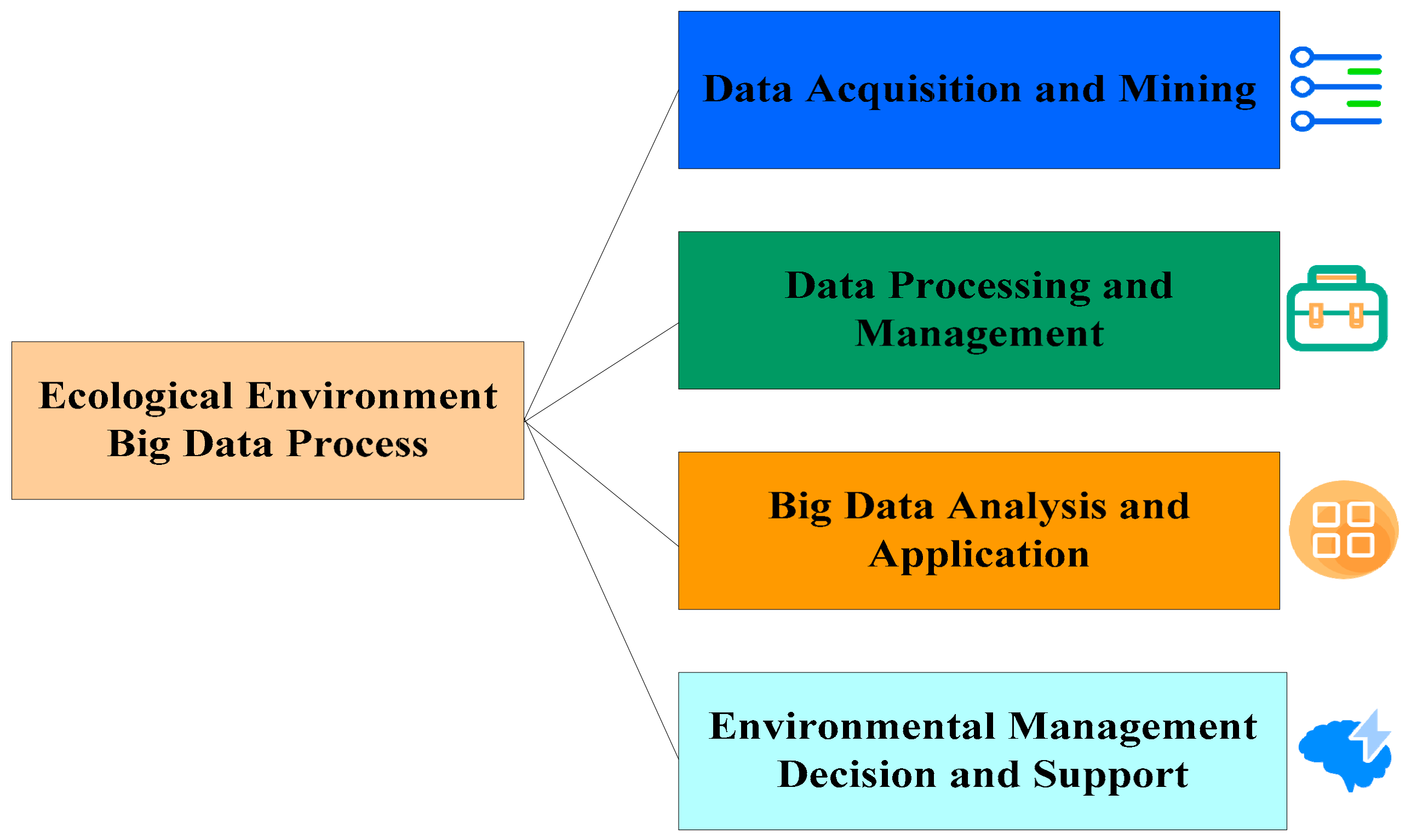
3.1.1. The Application Level of Ecological Environment Big Data

With the development of the Internet and the information industry, big data has become the focus of attention. In the field of ecological environment, due to the complexity of the ecological environment and the difficulty of supervision, it is difficult to deal with big data only by relying on the existing human and material resources [12,13]. The in-depth research and practice of big data has important practical significance for improving the level of environmental protection management and promoting decision support. Data collection is mainly to obtain multi-source heterogeneous spatiotemporal big data with complex sources, complex types, and wide data coverage [14,15]. Single-site data and continuous spatial distribution data provide the possibility for continuous time change monitoring of ecological environment big data [16]. The application level of ecological environment big data is shown in Figure 1.
It is important to monitor the environmental quality status and the trend of the change of environmental problems, find out the status of environmental pollution sources and the risks existing in the environment, and make risk predictions. The application of big data technology in environmental protection is conducive to the transformation of monitoring methods in the face of severe ecological environment conditions and environmental problems and is conducive to the formation of an integrated monitoring system combining point and surface, dynamic and dynamic, and sky and earth. It can be seen from Figure 1 that the four types of ecological environment big data application levels are: data information mining, data information processing, big data application, and environmental support management. The mining of data information includes monitoring, sensor data, Internet data, and sample surveys; the processing of data information includes data cleaning, fusion, management system, and data sharing; the data applications include system models, carrying capacity, machine learning, and cloud computing; the supporting management of the environment includes development strategies, goals, systems, and norms [17,18,19]. The main steps of environmental pollution assessment and analysis for economic loss and financial risk are shown in Figure 2.

3.1.2. Problems with AHP

The key to AHP is to construct a pairwise comparison matrix. The comparison between those who have a greater relationship between pairwise comparisons has the characteristics of simplicity and accuracy [20]. For example, comparing the pros and cons of things A, B, C, and D, if a pairwise comparison is made, the relationship between A and B, B and C can be quickly and accurately judged, so that the relationship between the four can be accurately judged through the pairwise comparison [21]. Therefore, the pairwise comparison between indicators is a key feature in the application of AHP.
The biggest problem faced by AHP in the application process is the consistency of the pairwise comparison matrix. Through pairwise comparison, a clear multiple relationship between any two indicators can be well established, but at the same time, it would also bring disadvantages to the pairwise comparison matrix. On the one hand, since the comparison results between the two indicators are always multiples of natural numbers, such as 1–9 (or the reciprocal of the corresponding natural numbers), the results obtained in this way are prone to human errors and reduce the accuracy. For example, x 12 = 4 / 5 , when judging, only a closer value can be selected from the two values of 1 or 1/2 that are relatively close, which would cause an error. On the other hand, since this multiple relationship is generated between pairs of indicators, when there are multiple indicators that need to be compared in pairs, the comparison results are likely to cause large deviations. This is due to the difference in the judge’s cognition of objective things, so that the obtained judgment results cannot make the pairwise comparison matrix have good consistency. For example, x 13 = 1 , and x 32 = 2 , then for a pairwise comparison matrix with complete consistency, there should be x 13 x 32 = x 12 = 2 , while the actual expert judgment may be assigned a value of x 12 = 1 / 2 . Therefore, it can be seen that the multiple relationship of the scale is also makes it easy to bring problems to the application of AHP. To perform data mining, there must be goals, then you define the appropriate key factors or hierarchical goals, and then perform data mining. This will shorten your digging time and increase your efficiency. In data mining, it is very important to build a cube, and the cube itself is a multi-layer structure. Thus, from these aspects, analytic hierarchy process and data mining can be used together.

3.1.3. Construction of Pairwise Comparison Judgment Matrix in AHP

In view of the multiple environmental accidents, the application of FAHP combined with AHP technology is more targeted and accurate for the decision-making of environmental accident emergency response plans. In the process of the original assignment of each element of the pairwise comparison judgment matrix, errors would occur, thus affecting the consistency of the pairwise comparison judgment matrix. However, each element value has a different influence on the consistency of the pairwise comparison judgment matrix, and the value with larger error tends to have a greater impact on the pairwise comparison judgment matrix [22]. The search process is as follows, and a fifth-order matrix is built first:
x 11 x 12 x 15 x 21 x 25 x 51 x 52 x 55
The pairwise comparison judgment matrix is:
x 11 = x 22 = x 33 = x 44 = x 55 = 1 x 12 = 1 / x 21 x 13 = 1 / x 31 x 45 = 1 / x 54
It can be seen from Formula (2) that as long as the upper half of the pairwise comparison judgment matrix satisfies complete consistency, the entire paired comparison judgment matrix satisfies complete consistency. Therefore, the full consistency adjustment of the upper half of the matrix can be achieved.
Through Formula (3):
x a q x q b = x a b
it can be seen that x 12 x 23 = x 13 , x 12 = x 13 / x 23 , and then it can be deduced: x 12 = x 14 / x 24 . From this, a vector of values of x 12 can be constructed:
x 12 = x 12 x 13 ¯ x 23 x 14 ¯ x 24 x 15 ¯ x 25
The vector values are then compared by averaging each value or by direct observation. A value or two values with a large difference are found, that is, a value that has a large impact on the complete consistency of the matrix [23]. If the value of x 14 / x 24 is an outlier, x 14 and x 24 are modified. At the same time, the value vectors of x 14 and x 24 are referenced accordingly, so that the value of x 14 / x 24 is the average or close to the average value of the remaining values of the x 12 -valued vector. The values of the x 12 -valued vector are then averaged to obtain a value of x 12 .
After the membership relationship is determined, different levels of judgment matrices can be constructed according to the criteria of the previous level [24]. The judgment matrix is formed as:
D = D a b m × m
m is the number of elements, and matrix D is called the positive and negative judgment matrix. If the matrix D has complete consistency, then there are:
D a q × D q b = D a b
Based on completing the established AHP structure model and constructing the comparative judgment matrix, the process of calculating the index weights by the AHP method before optimization can be understood first.
The premise of this process is the need to calculate the consistency index:
D A = ( α max m ) / m 1
then the value of the average random consistency index is shown in Table 1.
It can be known from Table 1 that when the random consistency ratio is D P = D A / P A < 0.1 , the results of the hierarchical single ordering have satisfactory consistency. If the index of layer H for single ordering is D A b , and the corresponding average random consistency index is D P b , then the total ordering ratio of layer H is:
P A = b = 1 m x b D A b b = 1 m x b D P b
It is compared with the calculation process before optimization, the process of calculating the weight of each index by the AHP after estimation has the characteristics of fast calculation process. In addition, the optimized AHP considers the key elements that affect the consistency of the judgment matrix when adjusting the judgment matrix, which makes the calculation result of the weight more scientific.

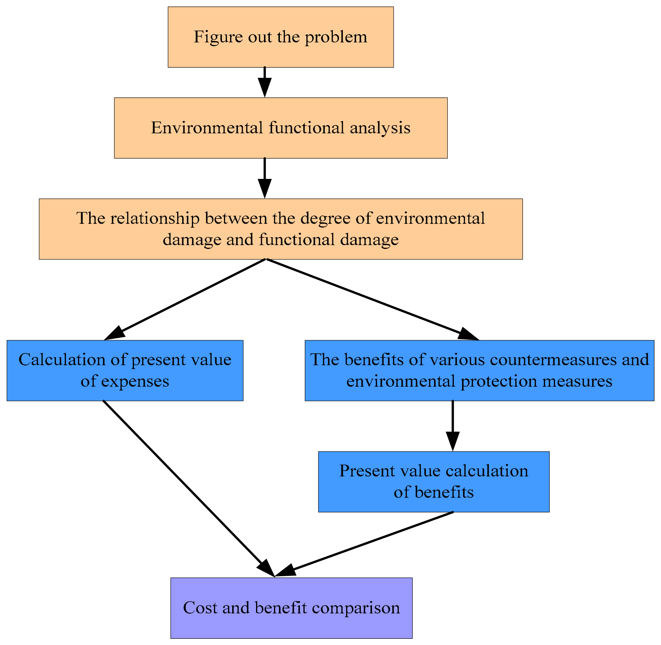
3.2. Evaluation of Environmental Pollution on Economic Loss and Financial Risk

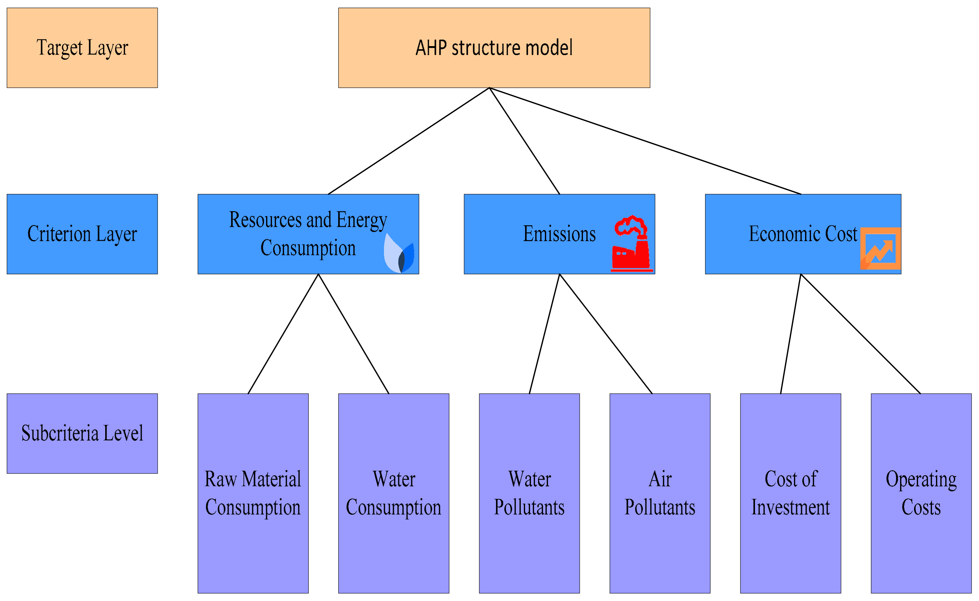
3.2.1. Establishment of Environmental Pollution Assessment Index System and Hierarchical Structure Model

AHP is used to evaluate the economic loss and financial risk of environmental pollution. It establishes an evaluation index system according to the characteristics to be evaluated and analyzes the hierarchical relationship between the established index systems; an AHP structure model is established, and an evaluation table is formulated based on the established index system and AHP structure model to evaluate and judge the importance relationship between each index in each index system. The comprehensive evaluation and judgment results construct a pairwise comparison judgment matrix. The weight of each indicator is calculated through the adjusted pairwise comparison judgment matrix, and the risk is assessed using the determined weight of each indicator and the data in actual operation of the technology. Figure 3 shows the specific steps of using AHP to evaluate the economic loss and financial risk of environmental pollution.
It can be seen from Figure 3 that the index hierarchy model is established by analyzing the steps in the index system. An example of an AHP structure model for environmental pollution economic loss and financial risk assessment is shown in Figure 4.

3.2.2. Construction of Comparative Judgment Matrix

A pairwise comparison matrix is constructed, and the element values in the matrix represent the pairwise comparison between the indicators of environmental pollution and economic loss. If the pollutant treatment in a certain area is taken as an example, the comparative judgment of the simulation is shown in Table 2.
According to Table 2, the comparison judgment matrix A can be constructed as:
X = x 11 x 12 x 13 x 21 x 22 x 23 x 31 x 32 x 33 = 2 5 4 1 4 2 4 1 3 1 5 2
Element x 12 = 5 in matrix X represents that the indicator of pollutant discharge is obviously important relative to the indicator of economic cost; element x 13 = 4 represents that the indicator of pollutant discharge is slightly more important than the indicator of financial risk; element x 23 = 4 represents that the indicator of economic cost is more important than the indicator of financial risk.

3.2.3. Risk Assessment Method

The weight of the index is determined by the entropy weight method. A positive indicator is an indicator that the warning value increases with the increase in the indicator value, and a negative indicator is an indicator that the warning value decreases when the indicator value increases:
Q x y = Q x y Q y min Q y max Q y min
Q x y = Q y max Q x y Q y max Q y min
Among them, Q x y represents the indicator value of the y -th indicator in the x -th phase, and Q y min represents the minimum value of the y -th indicator. Q y max represents the maximum value of the y -th index, and Q x y represents the standardized index value of the y -th index in the x -th phase. After the data standardization is completed, the weight of each index in each phase is determined, and the weight changes with the change of the time series:
R x y = Q x y x = 1 n Q x y
Among them, R x y represents the weight of the index value of the y -th index in the x -th phase in all phases, and Q x y represents the standardized index value:
e y = 1 ln n x = 1 n R x y ln R x y
g y = 1 e y
M y = g y y = 1 m g y
Among them, n is the length of the time series, and e y is the entropy value of the y -th index. g y represents the difference index of the y -th indicator, and M y represents the weight value of the y -th indicator.
The risk value is obtained according to the index weight and the standardized value of the index:
V x y = M y × Q x y
V x = y = 1 m V x y
Among them, V x y represents the risk value of the index value of the y -th index in the x -th phase, and V x represents the risk value in the x -th phase.

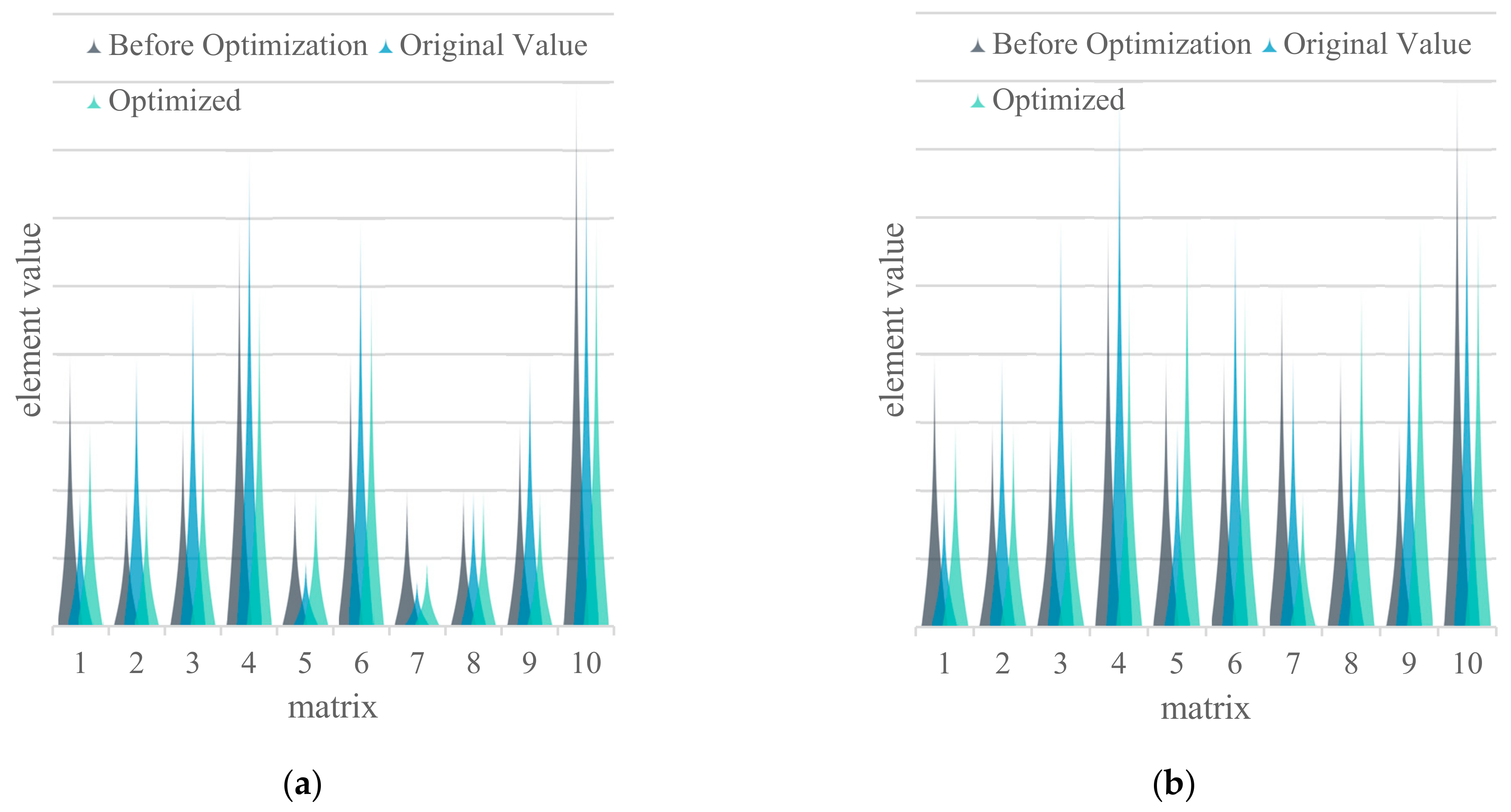
3.3. Comparison of Weight Calculation Results before and after the Improvement of AHP

The analytic hierarchy structure model of the comparison judgment matrix before optimization and the construction steps of the comparison judgment matrix are the same as the steps after optimization, so it is only necessary to calculate the following steps: α max = 3.0038 , and E = ( 0.648129 , 0.229517 , 0.122123 ) . The weights of the three indicators H 1 , H 2 , and H 3 in the judgment matrix are checked for consistency, and these are:
D A = α max m m 1 = 3.0038 3 3 1 = 0.0019
When m = 3 , the consistency index P A = 0.59 . The consistency ratio can be calculated as:
D P = D A P A = 0.0019 0.59 = 0.0032 < 0.1
then it can be seen that the judgment matrix X H has satisfactory consistency.
When m = 5 , the consistency index P A = 1.13 . The consistency ratio can be calculated as:
D P = D A P A = 0.0050 1.13 = 0.0044 < 0.1
then it can be seen that the judgment matrix H 1 D has satisfactory consistency.
The calculation process of the optimized AHP is relatively simple. A new matrix can be derived from the calculated weight values. The weight values of each index of the judgment matrix calculated by the AHP before and after optimization are compared with the original value of judgment, and the comparison results are shown in Figure 5.
It can be seen from Figure 5a that the values of each element of the judgment matrix X H calculated by the optimized AHP are relatively consistent with the original values judged by experts. It can be seen from Figure 5b that the values of each element of the judgment matrix X H and judgment matrix H 1 D calculated by the AHP before optimization are generally different from the original values judged by experts. That is to say, the element values calculated by the AHP before optimization deviate from the original judgment value, so that the judgment matrix has been adjusted to a certain extent as a whole. In the optimized AHP, except for the values of individual key elements that are adjusted, other calculated values are well consistent with the original judgment values.

4. Determination Experiment of Evaluating Financial Risk Index Weight Based on AHP

4.1. Checking of Consistency of Judgment Matrix

In the level defined by AHP, the specific scale quantification of the relative importance of each element compared with all other elements is shown in Table 3.
The consistency of the matrix is checked through the specific quantification in Table 3, and the logic of the previous pairwise matrices is judged. If there is a logical error, the matrix needs to be rebuilt. When the values of DA and DP are both less than 0.1, it is judged that the consistency of the pairwise matrices meets the requirements. The numerical look-up table of PA is shown in Table 4.
Figure 6 shows a summary of the calculation results of the eigenvectors and eigenvalues of each judgment matrix based on the consistency index in Table 4.
It can be seen from Figure 6a that the judgment matrix X H financial risk evaluation system α max = 4.1387 ; therefore, DA = 0 . 0411 , and DP = 0 . 051 ; the consistency test is passed. It can be seen from Figure 6b that the judgment matrix H 1 D financial risk evaluation system α max = 3.1495 ; therefore, DA = 0 . 0215 , and DP = 0 . 0357 ; the consistency test is passed. It can be seen from Figure 6c that the judgment matrix H 2 D financial risk evaluation system α max = 3.0395 ; therefore, DA = 0 . 0098 , and DP = 0 . 0266 . Finally, the comprehensive ranking of each index is calculated, and the weight coefficient of the financial risk evaluation index is summarized, as shown in Figure 7.
According to Figure 7, it is not difficult to see that for the ecological environment, the financial risk point of environmental pollution affecting economic capacity is the most important while from the perspective of primary indicators. From the perspective of secondary indicators, the comprehensive weight is as high as 22.63%. This indicator is a measure of economic loss, reflecting the consideration of economic costs. When there are financial risk points that affect economic efficiency, they should be paid attention to. In addition, when these evaluation indicators are in a bad state, the economic situation caused by the ecological environment would tend to deteriorate, and financial risks are more likely to occur.

4.2. Comparison of the Improved AHP Analysis Results

AHP analysis is to use a systematic structure to layer complex factors, and to analyze and evaluate the results step by step. When using AHP analysis, decision makers are only required to express the relative weights of two factors with a simple quantitative scale. For complex or difficult-to-define situations, it is difficult to express in a quantitative way. It is difficult for experts to directly give the corresponding numerical values when answering the questionnaire, and to analyze the weight of each risk factor. The difference between the results of fuzzy AHP and traditional AHP is compared, the weights and rankings of all risk factors are deduced by AHP, and then compared with the results of fuzzy AHP.
Since the previous risk criteria and risk factor consistency verification results show that the consistency test of each level is less than 0.1, the weight and ranking of each risk factor after the level is concatenated is obtained; the risk factors are classified into high-risk factor group (50%), moderate-risk factor group (30%) and low-risk factor group (30%), and then compared with the data of fuzzy analytic hierarchy process, respectively. The specific data results are shown in Figure 8.
It can be seen from Figure 8a that the weights and rankings of most high-risk factors have changed, but they are still in the high-risk range. The impact of air pollution category has been raised from the fifth place of risk in the fuzzy analytic hierarchy process to the first place of risk in the analytic hierarchy process, and this risk is usually ignored. It can be seen from Figure 8b that there is a gap between the risk intensity caused by water pollution in the AHP results and the actual situation. The risk of the water pollution category dropped from the 19th medium risk in the fuzzy analytic hierarchy process to the 12th medium risk in the analytic hierarchy process, which is far from the actual implementation experience. It can be known from Figure 8c that due to economic growth in recent years, the cost control for environmental pollution fluctuates greatly. When estimating risk costs, great attention is paid to the impact of environmental protection investments on project finances. Therefore, the weights and rankings evaluated by the fuzzy analytic hierarchy process are more in line with the actual market conditions.

4.3. Strategy Optimization for Economic Losses Caused by Environmental Pollution

4.3.1. Adjusting the Industrial Structure to Ensure the Reduction of Total Pollutant Discharge

Efforts should be made to adjust the industrial structure of the industry. It is necessary to completely change the coal-dominated energy structure and actively create conditions for the development and utilization of natural gas. It is also necessary to establish ecological agriculture and ecological breeding, so as to scientifically and rationally use pesticides, chemical fertilizers, and strengthen biological control.

4.3.2. Focusing on Controlling Water Pollution

First, a good job in the treatment of wastewater from key pollution sources should be performed. Then, the construction of urban environmental infrastructure should be strengthened, and the construction of sewage treatment plants should be accelerated. Thirdly, the new large and medium-sized projects should be strictly examined and approved, especially the environmental protection review and the “three simultaneous” system, and the generation of pollution sources should be strictly controlled. Finally, the technology of wastewater recycling and comprehensive utilization of waste should be promoted to reduce the total amount of wastewater discharge and the stockpile of solid waste in the city, thereby reducing the total amount of pollutant discharge.

4.3.3. Strengthening Environmental Science and Technology Research and Fostering the Development of the Environmental Protection Industry

It is necessary to seize the opportunity of deepening the reform of the scientific and technological system and establish an environmental science and technology innovation system. Then, it is necessary to focus on technical research on major environmental problems in combination with local actual conditions, such as water, air, solid waste and noise pollution prevention and control technology, ecological restoration technology, environmental bioengineering technology and monitoring technology. It is needed to improve the management system of the environmental protection industry and regulate the market of the environmental protection industry. It is also necessary to mobilize the enthusiasm of social participation. The world’s environmental protection technologies should be actively introduced, digested, and absorbed to promote the harmonious development of the ecological environment and the economy. The key is to accelerate the complete set, serialization, and standardization of environmental protection products, so that the environmental protection industry would become a growth point of the national economy. We will strengthen the publicity and popularization of knowledge related to the application of big data on environmental pollution prevention and control and raise the public’s awareness of responsibility. In view of the public’s poor understanding of environmental big data, the government and environmental protection departments should do a good job in publicity and education, actively publicize the significance and application methods of environmental big data to the public and improve the public’s understanding of environmental big data.

5. Conclusions

With the application of big data technology in all walks of life playing an important role, the government’s protection of the ecological environment can better highlight its social value and economic benefits. Therefore, it has important theoretical and practical significance to apply the methods and technologies of big data to ecological environment governance. In order to better control the economic loss caused by environmental pollution, this paper analyzed the environmental pollution assessment index system and hierarchical structure model in detail and proposed the analytic hierarchy process to analyze the economic loss and predict the risk assessment. In order to verify the risk factors of AHP, a simulation comparison experiment was carried out in the experiment. Through experiments, it was found that the fuzzy analytic hierarchy process not only has a higher accuracy rate, but also is more in line with the actual market situation. Due to the complexity, difficulty and exploratory nature of the research on economic loss assessment of environmental pollution, it is still a new attempt to assess the economic loss of regional environmental pollution. Under the current international conditions, big data technology should be used to establish an environmental value assessment index system, so that the assessment of environmental pollution and economic losses in various regions can be carried out as soon as possible in practice. Of course, in-depth research should be conducted in the follow-up, and a unified environmental pollution loss assessment method should be established according to the specific conditions of the region.

Author Contributions

Both L.W. and Y.S. designed and performed the experiment and prepared this manuscript. All authors have read and agreed to the published version of the manuscript.

Funding

The author(s) received no financial support for the research, authorship, and/or publication of this article.

Institutional Review Board Statement

Not applicable.

Informed Consent Statement

Not applicable.

Data Availability Statement

The data that support the findings of this study are available from the corresponding author upon reasonable request.

Conflicts of Interest

The authors declare no conflict of interest.

References

  1. Fan, S.; Xu, Y.Y. A Study on the Impact of Tourism Resources Development on Ecological Environment. Rev. Fac. Ing. 2017, 32, 375–384. [Google Scholar]
  2. Tang, D.; Liu, X.; Zou, X. An improved method for integrated ecosystem health assessments based on the structure and function of coastal ecosystems: A case study of the Jiangsu coastal area, China. Ecol. Indic. 2018, 84, 82–95. [Google Scholar] [CrossRef]
  3. Yang, Z. The EEWRS-based regional ecological environment water resource allocation model. J. Mine Vent. Soc. S. Afr. 2020, 73, 212–216. [Google Scholar]
  4. Zhao, D. Choice of Environmental and Economic Path for Building a Supply Chain Financial Cloud Ecosystem under the Background of “Internet +”. Wirel. Commun. Mob. Comput. 2021, 2021, 5597244. [Google Scholar] [CrossRef]
  5. Limbong, R.P.; Syah, T.; Anindita, R.; Moelyono. Risk Management for Start-Up Company: A Case Study of Healthy Kitchen Restaurant and Catering. Russ. J. Agric. Soc.-Econ. Sci. 2019, 86, 267–272. [Google Scholar] [CrossRef]
  6. Zhao, F.; Zhang, L.Y.; Zhao, M.M.; Shao, R.; Xu, M. Architecture and technical exploration of big data platform for ecological environment. Chin. J. Ecol. 2017, 36, 824–832. [Google Scholar]
  7. Chen, Y.; Chi, Y. Harnessing Structures in Big Data via Guaranteed Low-Rank Matrix Estimation. IEEE Signal Process. Mag. 2018, 35, 14–31. [Google Scholar] [CrossRef]
  8. Zheng, Q. Discussion on the Application of Geographic Information System in Urban Ecological Environment Management under the Background of Big Data. Open Access Libr. J. 2020, 7, 1–7. [Google Scholar] [CrossRef]
  9. Mo, T. Design of international financial risk estimation model based on improved genetic algorithm. J. Intell. Fuzzy Syst. 2021, 737, 189936. [Google Scholar] [CrossRef]
  10. Wu, C.; Zapevalova, E.; Chen, Y.; Li, F. Time Optimization of Multiple Knowledge Transfers in the Big Data Environment. Comput. Mater. Contin. 2018, 54, 269–285. [Google Scholar]
  11. Que, W.; Zhang, Y.; Liu, S.; Yang, C. The spatial effect of fiscal decentralization and factor market segmentation on environmental pollution. J. Clean. Prod. 2018, 184, 402–413. [Google Scholar] [CrossRef]
  12. Nasir, M.; Al-Masri, A.N. Multi-source Heterogeneous Ecological Big Data Adaptive Fusion Method Based on Symmetric Encryption. Fusion Pract. Appl. 2021, 5, 8–20. [Google Scholar] [CrossRef]
  13. Hsieh, Y.; Lo, Y. Understanding Customer Motivation to Share Information in Social Commerce. J. Organ. End User Comput. 2021, 33, 1–26. [Google Scholar] [CrossRef]
  14. Bttger, T.; Cuadrado, F.; Tyson, G.; Castro, I.; Uhlig, S. Open Connect Everywhere: A Glimpse at the Internet Ecosystem through the Lens of the Netflix CDN. Acm Sigcomm Comput. Commun. Rev. 2018, 48, 28–34. [Google Scholar] [CrossRef]
  15. Nie, S.; Wang, A.; Yuan, Y. Comparison of clinicopathological parameters, prognosis, micro-ecological environment and metabolic function of Gastric Cancer with or without Fusobacterium sp. Infection. J. Cancer 2021, 12, 1023–1032. [Google Scholar] [CrossRef]
  16. Lee, J.H.; Park, J.S.; Choi, S. Environmental influence in the forested area toward human health: Incorporating the ecological environment into art psychotherapy. J. Mt. Sci. 2020, 17, 992–1000. [Google Scholar] [CrossRef]
  17. Chen, C.; Chen, C.W.K. Performance Assessment on Campus Ecological Environment. J. Environ. Prot. Ecol. 2020, 21, 893–900. [Google Scholar]
  18. Liu, Q.; Sun, S.; Rong, B.; Kadoch, M. Intelligent Reflective Surface Based 6G Communications for Sustainable Energy Infrastructure. IEEE Wirel. Commun. Mag. 2021, 28, 49–55. [Google Scholar] [CrossRef]
  19. Rajendran, S.; Khalaf, O.I.; Alotaibi, Y.; Alghamdi, S. MapReduce-based big data classification model using feature subset selection and hyperparameter tuned deep belief network. Sci. Rep. 2021, 11, 24138. [Google Scholar] [CrossRef]
  20. Silva, F. Fiscal Deficits, Bank Credit Risk, and Loan Loss Provisions. J. Financ. Quant. Anal. 2021, 56, 1537–1589. [Google Scholar] [CrossRef]
  21. St-Hilaire, W.A.; Boisselier, P. Evaluating profitability strategies and the determinants of the risk performance of sectoral and banking institutions. J. Econ. Adm. Sci. 2018, 34, 174–186. [Google Scholar] [CrossRef]
  22. Dyk, J.V.; Lange, J.; Vuuren, G.V. The impact of systemic loss given default on economic capital. Int. Bus. Econ. Res. J. 2017, 16, 87–100. [Google Scholar]
  23. Lukuyu, J.M.; Blanchard, R.E.; Rowley, P.N. A risk-adjusted techno-economic analysis for renewable-based milk cooling in remote dairy farming communities in East Africa. Renew. Energy 2018, 130, 700–713. [Google Scholar] [CrossRef] [Green Version]
  24. Lim, S.-M. A Study on University Student’s Recognition of Physical Education by IPA. Korean J. Phys. Educ. 2017, 56, 125–138. [Google Scholar] [CrossRef]
Figure 1. The application level of ecological environment big data.
Sustainability 15 03834 g001
Figure 2. Basic steps of environmental pollution for economic cost and risk assessment.
Sustainability 15 03834 g002
Figure 3. The steps of environmental pollution economic loss and financial risk assessment.
Sustainability 15 03834 g003
Figure 4. Hierarchical structure of indicators of AHP structure model.
Sustainability 15 03834 g004
Figure 5. Comparison of the calculated value of each element of judgment matrix X H and judgment matrix H 1 D with the original value. (a) Judgment matrix X H ; (b) judgment matrix.
Sustainability 15 03834 g005
Figure 6. Weight calculation results of judgment matrix X H , judgment matrix H 1 D and judgment matrix H 2 D . (a) Calculation result of judgment matrix X H ; (b) calculation result of judgment matrix H 1 D ; (c) calculation result of judgment matrix H 2 D .
Sustainability 15 03834 g006
Figure 7. Weight coefficients of financial risk evaluation indicators.
Sustainability 15 03834 g007
Figure 8. Comparison of high, medium, and low risk intensity of AHP analysis results. (a) High-risk factor; (b) medium-risk factor; (c) low-risk factor.
Sustainability 15 03834 g008
Table 1. Average stochastic consistency metrics.
M123456
PA00.130.550.891.131.36
Table 2. Financial risk assessment table of pollutants in a certain region.
First-Level Index Evaluation Table
EmissionsEconomic CostFinancial Risk
Emissions254
Economic Cost1/424
Financial Risk1/31/52
Table 3. 1–10 scaling metrics table.
DefinitionImportance
The A factor is as important as the B factor2
The A factor is slightly more important than the B factor4
The A factor is considerably more important than the B factor6
The A factor is significantly more important than the B factor8
The A factor is absolutely more important than the B factor10
The degree of importance is in the middle of the above cases1, 3, 5, 7, 9
Table 4. Average random consistency index PA value table.
Order345678910
PA0.490.861.231.421.531.571.591.64
Disclaimer/Publisher’s Note: The statements, opinions and data contained in all publications are solely those of the individual author(s) and contributor(s) and not of MDPI and/or the editor(s). MDPI and/or the editor(s) disclaim responsibility for any injury to people or property resulting from any ideas, methods, instructions or products referred to in the content.

