
Spatiotemporal Patterns of Evapotranspiration in Central Asia from 2000 to 2020


Abstract
1. Introduction
2. Data and Methods
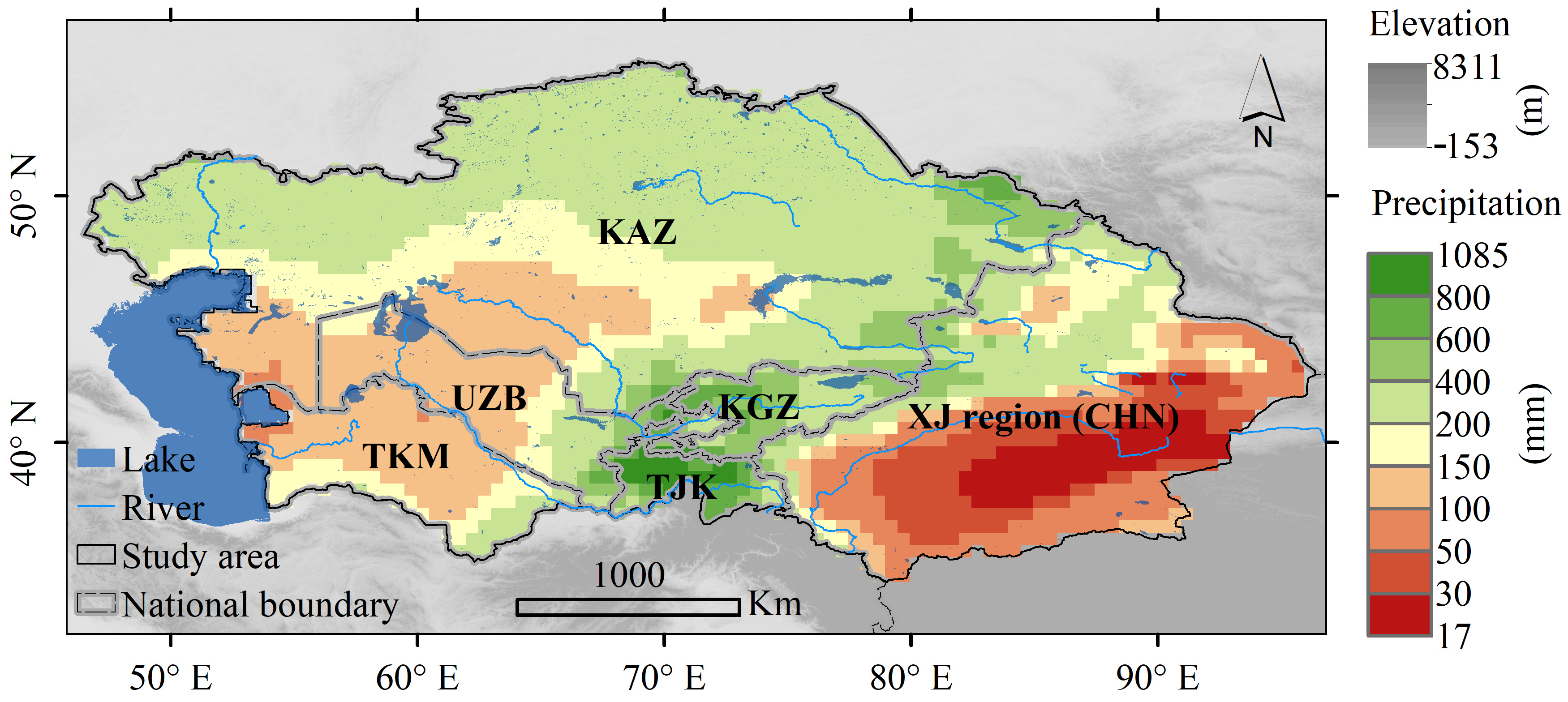
2.1. Study Area
2.2. Data Sources
2.3. Methods
2.3.1. Algorithm of ET and PET
2.3.2. Attribution of ET Changes
2.3.3. Trend Analysis
3. Results
3.1. Changing Trend of ET and PET
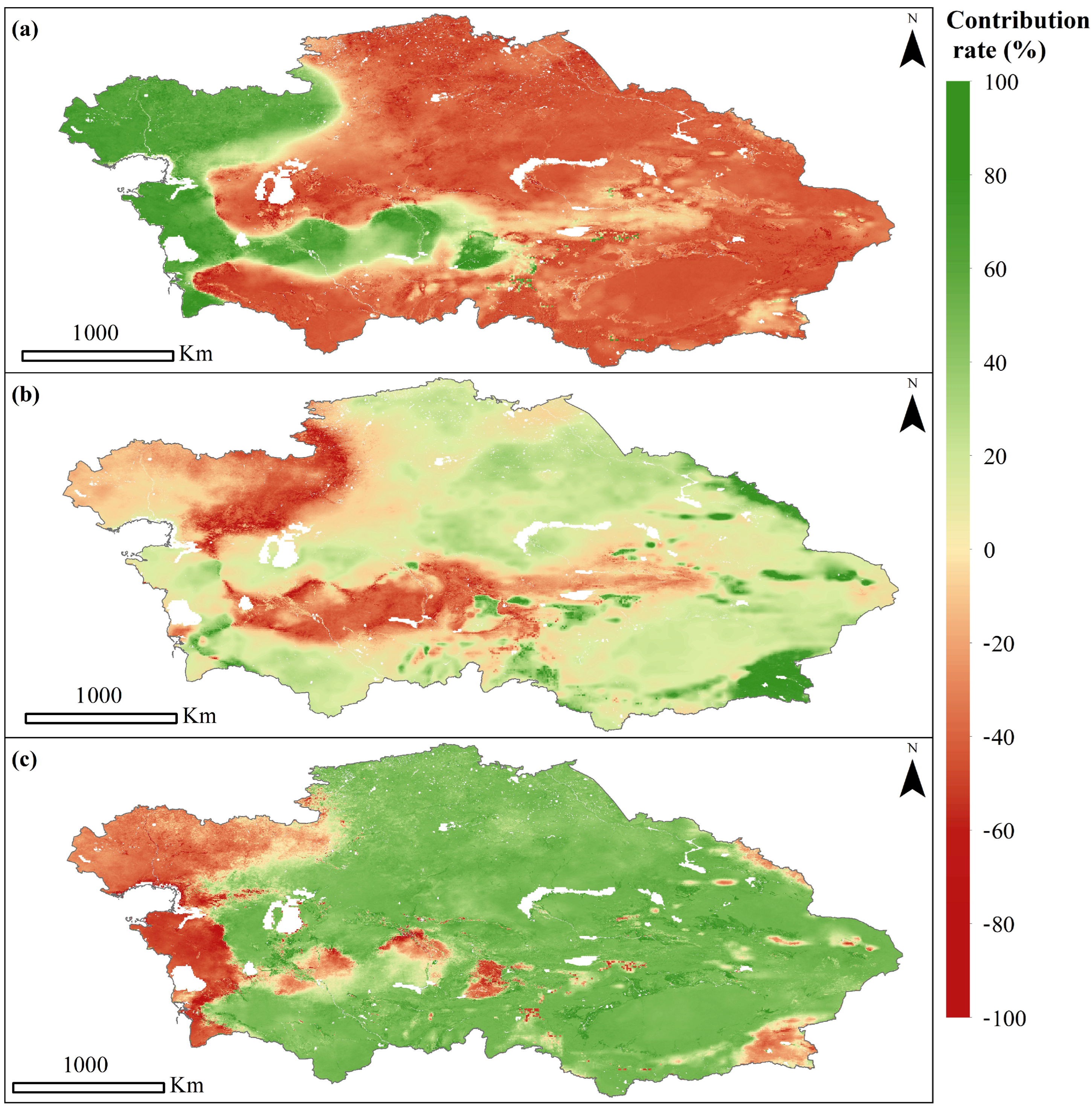
3.2. Attribution of ET Trend
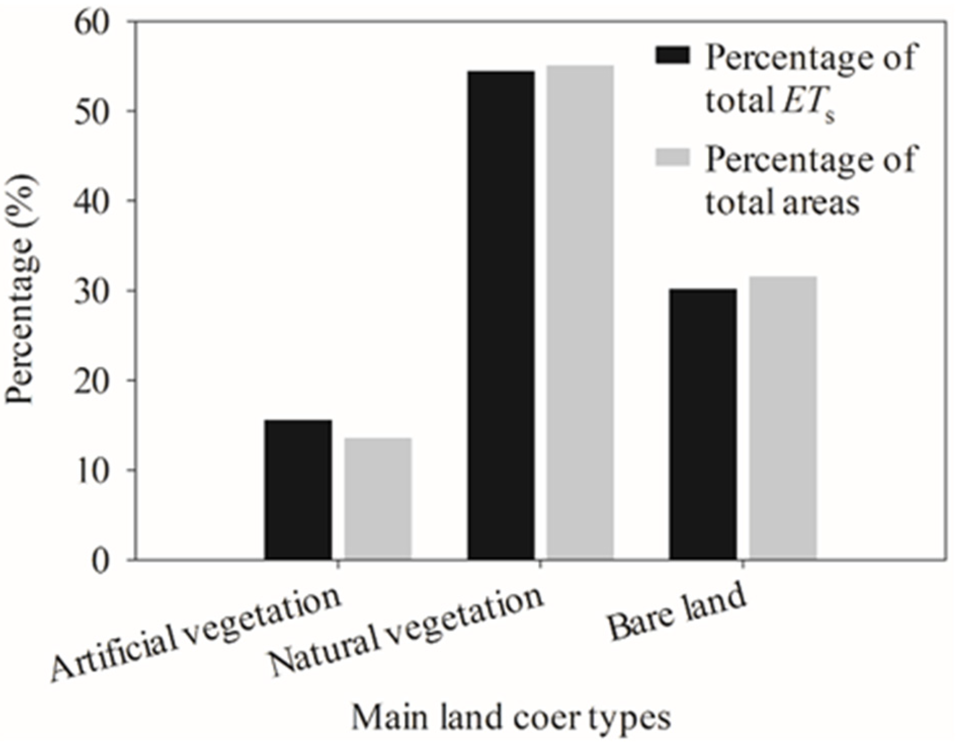
3.3. Contribution of Soil Evaporation and Transpiration to ET Change
4. Discussion
4.1. Driving Forces of ET Variation in Arid Region
4.2. Effects of PET on ET
4.3. Effects of Soil Evaporation and Mitigation Measures
5. Conclusions
Author Contributions
Funding
Data Availability Statement
Acknowledgments
Conflicts of Interest
Appendix A
- ET estimation and validation

| Parameter | Description | Equation |
|---|---|---|
| ET | Evapotranspiration | |
| ETc | Vegetation transpiration | |
| ETs | Soil evaporation | |
| ETi | Vegetation interception evaporation | |
| ETws | Wet soil surface evaporation | |
| fv | Fraction of green vegetation in the scene | |
| fT | Plant temperature constraint | |
| fsm | Soil moisture constraint | |
| fwet | Relative surface wetness | |
| Lu | Upward long wave radiation | |
| Ld | Downward long wave radiation | |
| εa | Atmospheric emissivity | |
| Rn | Net radiation | |
| Rnc | Net radiation to the vegetation | |
| Rns | Net radiation to the soil |

- Contribution rate of human activities and climate factors to NDVI
References
- Liu, B.; Henderson, M.; Zhang, Y.; Ming, X. Spatiotemporal change in China’s climatic growing season: 1955–2000. Clim. Chang. 2010, 99, 93–118. [Google Scholar] [CrossRef]
- Hajimirzajan, A.; Vahdat, M.; Sadegheih, A.; Shadkam, E.; Bilali, H.E. An integrated strategic framework for large-scale crop planning: Sustainable climate-smart crop planning and agri-food supply chain management. Sustain. Prod. Consum. 2020, 26, 709–732. [Google Scholar] [CrossRef]
- Peng, Y. Possible Underlying Mechanisms of Severe Decadal Droughts in Arid Central Asia During the Last 530 Years: Results From the Last Millennium Climate Reanalysis Project Version 2.0. J. Geophys. Res. Atmos. 2021, 126, e2020JD033409. [Google Scholar] [CrossRef]
- Khaydar, D.; Chen, X.; Huang, Y.; Ilkhom, M.; Liu, T.; Friday, O.; Farkhod, A.; Khusen, G.; Gulkaiyr, O. Investigation of crop evapotranspiration and irrigation water requirement in the lower Amu Darya River Basin, Central Asia. J. Arid. Land 2021, 13, 17. [Google Scholar] [CrossRef]
- Li, T.; Xia, J.; Zhang, L.; She, D.; Wang, G.; Cheng, L. An improved complementary relationship for estimating evapotranspiration attributed to climate change and revegetation in the Loess Plateau, China. J. Hydrol. 2021, 592, 125516. [Google Scholar] [CrossRef]
- Yang, L.; Feng, Q.; Zhu, M.; Wang, L.; Alizadeh, M.R.; Adamowski, J.F.; Wen, X.; Yin, Z. Variation in actual evapotranspiration and its ties to climate change and vegetation dynamics in northwest China. J. Hydrol. 2022, 607, 127533. [Google Scholar] [CrossRef]
- Banerjee, S.; Biswas, B. Assessing Climate Change Impact on Future Reference Evapotranspiration Pattern of West Bengal, India. Agric. Sci. 2020, 11, 793–802. [Google Scholar] [CrossRef]
- Zhu, G.F.; Zhang, K.; Li, X.; Liu, S.M.; Ding, Z.Y.; Ma, J.Z.; Huang, C.L.; Han, T.; He, J.H. Evaluating the complementary relationship for estimating evapotranspiration using the multi-site data across north China. Agric. For. Meteorol. 2016, 230–231, 33–44. [Google Scholar] [CrossRef]
- Sánchez, J.M.; López-Urrea, R.; Valentín, F.; Caselles, V.; Galve, J.M. Lysimeter assessment of the Simplified Two-Source Energy Balance model and eddy covariance system to estimate vineyard evapotranspiration. Agric. For. Meteorol. 2019, 274, 172–183. [Google Scholar] [CrossRef]
- Luan, P.V.; Eugenio, F.C.; Filgueiras, R.; Cunha, F.; Mantovani, E.C. Mapping within-field variability of soybean evapotranspiration and crop coefficient using the Earth Engine Evaporation Flux (EEFlux) application. PLoS ONE 2020, 15, e0235620. [Google Scholar]
- Marin, F.R.; Angelocci, L.R.; Nassif, D.; Vianna, M.S.; Carvalho, K.S. Revisiting the crop coefficient-reference evapotranspiration procedure for improving irrigation management. Theor. Appl. Climatol. 2019, 138, 1785–1793. [Google Scholar] [CrossRef]
- Paciolla, N.; Corbari, C.; Hu, G.; Zheng, C.; Mancini, M. Evapotranspiration estimates from an energy-water-balance model calibrated on satellite land surface temperature over the Heihe basin. J. Arid. Environ. 2021, 188, 104466. [Google Scholar] [CrossRef]
- Denager, T.; Looms, M.C.; Sonnenborg, T.O.; Jensen, K.H. Comparison of evapotranspiration estimates using the water balance and the eddy covariance methods. Vadose Zone J. 2020, 19. [Google Scholar] [CrossRef]
- Elkatoury, A.; Alazba, A.A.; Mossad, A. Estimating Evapotranspiration Using Coupled Remote Sensing and Three SEB Models in an Arid Region. Environ. Process. 2020, 7, 109–133. [Google Scholar] [CrossRef]
- Senkondo, W.; Munishi, S.E.; Tumbo, M.; Nobert, J.; Lyon, S.W. Comparing Remotely-Sensed Surface Energy Balance Evapotranspiration Estimates in Heterogeneous and Data-Limited Regions: A Case Study of Tanzania’s Kilombero Valley. Remote Sens. 2019, 11, 1289. [Google Scholar] [CrossRef]
- Yao, Y.J.; Liang, S.L.; Zhou, G.Y.; Li, Y.L. MODIS-driven estimation of terrestrial latent heat flux in China based on a modified Priestley–Taylor algorithm. Agric. For. Meteorol. 2013, 171–172, 187–202. [Google Scholar] [CrossRef]
- Brutsaert, W. A generalized complementary principle with physical constraints for land-surface evaporation. Water Resour. Res. 2016, 51, 8087–8093. [Google Scholar] [CrossRef]
- Feng, S.; Liu, J.; Zhang, Q.; Zhang, Y.; Sun, P. A global quantitation of factors affecting evapotranspiration variability. J. Hydrol. 2020, 584, 124688. [Google Scholar] [CrossRef]
- Ning, T.; Li, Z.; Feng, Q.; Qin, Y. Attribution of growing season evapotranspiration variability considering snowmelt and vegetation changes in the arid alpine basins. Hydrol. Earth Syst. Sci. 2021, 25, 3455–3469. [Google Scholar] [CrossRef]
- Hu, S.; Mo, X. Attribution of Long-Term Evapotranspiration Trends in the Mekong River Basin with a Remote Sensing-Based Process Model. Remote Sens. 2021, 13, 303. [Google Scholar] [CrossRef]
- Hu, Z.; Zhang, C.; Hu, Q.; Tian, H. Temperature Changes in Central Asia from 1979 to 2011 Based on Multiple Datasets. J. Clim. 2014, 27, 1143–1167. [Google Scholar] [CrossRef]
- Zhu, X.; Wei, Z.; Dong, W.; Ji, Z.; Chen, D. Dynamical downscaling simulation and projection for mean and extreme temperature and precipitation over central Asia. Clim. Dyn. 2020, 54, 3279–3306. [Google Scholar] [CrossRef]
- Hao, X.; Chen, Y.; Xu, C.; Li, W. Impacts of Climate Change and Human Activities on the Surface Runoff in the Tarim River Basin over the Last Fifty Years. Water Resour. Manag. 2008, 22, 1159–1171. [Google Scholar] [CrossRef]
- Su, Y.; Li, X.; Feng, M.; Nian, Y.; Huang, L.; Xie, T.; Zhang, K.; Chen, F.; Huang, W.; Chen, J. High agricultural water consumption led to the continued shrinkage of the Aral Sea during 1992–2015. Sci. Total Environ. 2021, 777, 145993. [Google Scholar] [CrossRef] [PubMed]
- Deliry, S.I.; Avdan, Z.Y.; Do, N.T.; Avdan, U. Assessment of human-induced environmental disaster in the Aral Sea using Landsat satellite images. Environ. Earth Sci. 2020, 79, 471. [Google Scholar] [CrossRef]
- Chen, F.-H.; Chen, J.-H.; Holmes, J.; Boomer, I.; Austin, P.; Gates, J.B.; Wang, N.-L.; Brooks, S.J.; Zhang, J.-W. Moisture changes over the last millennium in arid central Asia: A review, synthesis and comparison with monsoon region. Quat. Sci. Rev. 2010, 29, 1055–1068. [Google Scholar] [CrossRef]
- Li, Z.; Chen, Y.; Fang, G.; Li, Y. Multivariate assessment and attribution of droughts in Central Asia. Sci. Rep. 2017, 7, 1316. [Google Scholar] [CrossRef]
- Chen, H.; Liu, H.; Chen, X.; Qiao, Y. Analysis on impacts of hydro-climatic changes and human activities on available water changes in Central Asia. Sci. Total Environ. 2020, 737, 139779. [Google Scholar] [CrossRef]
- Zeng, Z.; Piao, S.; Li, L.Z.X.; Zhou, L.; Ciais, P.; Wang, T.; Li, Y.; Lian, X.; Wood, E.F.; Friedlingstein, P.; et al. Climate mitigation from vegetation biophysical feedbacks during the past three decades. Nat. Clim. Change 2017, 7, 432–436. [Google Scholar] [CrossRef]
- Hao, X.; Zhang, S.; Li, W.; Duan, W.; Fang, G.; Ying, Z.; Guo, B. The Uncertainty of Penman-Monteith Method and the Energy Balance Closure Problem. J. Geophys. Res. Atmos. 2018, 123, 7433–7443. [Google Scholar] [CrossRef]
- Allen, R.G. Crop Evapotranspiration-Guidelines for computing crop water requirements. FAO Irrig. Drain. Pap. (FAO) 1998, 56, D05109. [Google Scholar]
- Ullah, S.; You, Q.; Ullah, W.; Ali, A. Observed changes in precipitation in China-Pakistan economic corridor during 1980–2016. Atmos. Res. 2018, 210, 1–14. [Google Scholar] [CrossRef]
- Arrieta-Castro, M.; Donado-Rodríguez, A.; Acua, G.J.; Canales, F.A.; Kamierczak, B. Analysis of Streamflow Variability and Trends in the Meta River, Colombia. Water 2020, 12, 1451. [Google Scholar] [CrossRef]
- Zhang, D.; Liu, X.; Zhang, L.; Zhang, Q.; Gan, R.; Li, X. Attribution of Evapotranspiration Changes in Humid Regions of China from 1982 to 2016. J. Geophys. Res. Atmos. 2020, 125, 1451. [Google Scholar] [CrossRef]
- Li, Z.; Chen, Y.; Yang, J.; Wang, Y. Potential evapotranspiration and its attribution over the past 50years in the arid region of Northwest China. Hydrol. Process. 2014, 28, 1025–1031. [Google Scholar] [CrossRef]
- Vadeboncoeur, M.A.; Green, M.B.; Heidi, A.; Campbell, J.L.; Beth, A.M.; Boyer, E.W.; Burns, D.A.; Fernandez, I.J.; Mitchell, M.J.; Shanley, J.B. Systematic variation in evapotranspiration trends and drivers across the Northeastern United States. Hydrol. Process. 2018, 32, 3547–3560. [Google Scholar] [CrossRef]
- Hu, D.; Xu, M.; Kang, S.; Wu, H. Impacts of climate change and human activities on runoff changes in the Ob River Basin of the Arctic region from 1980 to 2017. Theor. Appl. Climatol. 2022, 148, 1663–1674. [Google Scholar] [CrossRef]
- Wang, Y.; Gu, X.; Yang, G.; Yao, J.; Liao, N. Impacts of climate change and human activities on water resources in the Ebinur Lake Basin, Northwest China. J. Arid. Land 2021, 13, 18. [Google Scholar] [CrossRef]
- Zhou, H.; Chen, Y.; Hao, X.; Zhao, Y.; Fang, G.; Yang, Y. Tree rings: A key ecological indicator for reconstruction of groundwater depth in the lower Tarim River, Northwest China. Ecohydrology 2019, 12, e2142. [Google Scholar] [CrossRef]
- Hao, X.; Li, W. Impacts of ecological water conveyance on groundwater dynamics and vegetation recovery in the lower reaches of the Tarim River in northwest China. Environ. Monit. Assess. 2014, 186, 7605. [Google Scholar] [CrossRef]
- Chen, H.; Zhang, W.; Shalamzari, M.J. Remote detection of human-induced evapotranspiration in a regional system experiencing increased anthropogenic demands and extreme climatic variability. Int. J. Remote Sens. 2019, 40, 1887–1908. [Google Scholar] [CrossRef]
- Zou, M.; Niu, J.; Kang, S.; Li, X.; Lu, H. The contribution of human agricultural activities to increasing evapotranspiration is significantly greater than climate change effect over Heihe agricultural region. Sci. Rep. 2017, 7, 8805. [Google Scholar] [CrossRef]
- Wu, Y. Impacts of Human Activities on the Variations in Terrestrial Water Storage of the Aral Sea Basin. Remote Sens. 2021, 13. [Google Scholar]
- Yang, P.; Xia, J.; Zhan, C.; Chen, X.; Qiao, Y.; Chen, J. Separating the impacts of climate change and human activities on actual evapotranspiration in Aksu River Basin ecosystems, Northwest China. Nord. Hydrol. 2018, 49, 1740–1752. [Google Scholar] [CrossRef]
- Li, W.; Huang, F.; Shi, F.; Wei, X.; Zamanian, K.; Zhao, X. Human and climatic drivers of land and water use from 1997 to 2019 in Tarim River basin, China. Int. Soil Water Conserv. Res. 2021, 9, 532–543. [Google Scholar] [CrossRef]
- Zhao, Y.; Xue, J.; Wu, N.; Hill, R.L. An Artificial Oasis in a Deadly Desert: Practices and Enlightenments. Water 2022, 14, 2237. [Google Scholar] [CrossRef]
- Du, Q.; Zhang, M.; Wang, S.; Che, C.; Rong, M.; Ma, Z. Changes in air temperature over China in response to the recent global warming hiatus. J. Geogr. Sci. 2019, 29, 21. [Google Scholar] [CrossRef]
- Dong, Q.; Wang, W.; Shao, Q.; Xing, W.; Ding, Y.; Fu, J. The response of reference evapotranspiration to climate change in Xinjiang, China: Historical changes, driving forces, and future projections. Int. J. Climatol. 2020, 40, 235–254. [Google Scholar] [CrossRef]
- Fisher, J.B.; Tu, K.P.; Baldocchi, D.D. Global estimates of the land–atmosphere water flux based on monthly AVHRR and ISLSCP-II data, validated at 16 FLUXNET sites. Remote Sens. Environ. 2008, 112, 901–919. [Google Scholar] [CrossRef]
- Cao, M.; Wang, W.; Xing, W.; Wei, J.; Chen, X.; Li, J.; Shao, Q. Multiple sources of uncertainties in satellite retrieval of terrestrial actual evapotranspiration. J. Hydrol. 2021, 601, 126642. [Google Scholar] [CrossRef]
- Mu, Q.; Zhao, M.; Running, S.W. Improvements to a MODIS global terrestrial evapotranspiration algorithm. Remote Sens. Environ. 2011, 115, 1781–1800. [Google Scholar] [CrossRef]
- Zhang, Y.; Leuning, R.; Hutley, L.B.; Beringer, J.; McHugh, I.; Walker, J.P. Using long-term water balances to parameterize surface conductances and calculate evaporation at 0.05 spatial resolution. Water Resour. Res. 2010, 46, 5. [Google Scholar] [CrossRef]
- Zhang, Y. PML_V2 Global Evapotranspiration and Gross Primary Production (2002.07–2019.08). National Tibetan Plateau/Third Pole Environment Data Center. 2020. Available online: https://data.tpdc.ac.cn/en/data/48c16a8d-d307-4973-abab-972e9449627c/ (accessed on 26 October 2022).
- Zhang, Y.; Kong, D.; Gan, R.; Chiew, F.H.; McVicar, T.R.; Zhang, Q.; Yang, Y. Coupled estimation of 500 m and 8-day resolution global evapotranspiration and gross primary production in 2002–2017. Remote Sens. Environ. 2019, 222, 165–182. [Google Scholar] [CrossRef]


Disclaimer/Publisher’s Note: The statements, opinions and data contained in all publications are solely those of the individual author(s) and contributor(s) and not of MDPI and/or the editor(s). MDPI and/or the editor(s) disclaim responsibility for any injury to people or property resulting from any ideas, methods, instructions or products referred to in the content. |
© 2023 by the authors. Licensee MDPI, Basel, Switzerland. This article is an open access article distributed under the terms and conditions of the Creative Commons Attribution (CC BY) license (https://creativecommons.org/licenses/by/4.0/).
Share and Cite
Hao, X.; Fan, X.; Zhao, Z.; Zhang, J. Spatiotemporal Patterns of Evapotranspiration in Central Asia from 2000 to 2020. Remote Sens. 2023, 15, 1150. https://doi.org/10.3390/rs15041150
Hao X, Fan X, Zhao Z, Zhang J. Spatiotemporal Patterns of Evapotranspiration in Central Asia from 2000 to 2020. Remote Sensing. 2023; 15(4):1150. https://doi.org/10.3390/rs15041150
Chicago/Turabian StyleHao, Xingming, Xue Fan, Zhuoyi Zhao, and Jingjing Zhang. 2023. "Spatiotemporal Patterns of Evapotranspiration in Central Asia from 2000 to 2020" Remote Sensing 15, no. 4: 1150. https://doi.org/10.3390/rs15041150
APA StyleHao, X., Fan, X., Zhao, Z., & Zhang, J. (2023). Spatiotemporal Patterns of Evapotranspiration in Central Asia from 2000 to 2020. Remote Sensing, 15(4), 1150. https://doi.org/10.3390/rs15041150