FASSD: A Feature Fusion and Spatial Attention-Based Single Shot Detector for Small Object Detection

Abstract

Deep learning methods have significantly improved object detection performance, but small object detection remains an extremely difficult and challenging task in computer vision. We propose a feature fusion and spatial attention-based single shot detector (FASSD) for small object detection. We fuse high-level semantic information into shallow layers to generate discriminative feature representations for small objects. To adaptively enhance the expression of small object areas and suppress the feature response of background regions, the spatial attention block learns a self-attention mask to enhance the original feature maps. We also establish a small object dataset (LAKE-BOAT) of a scene with a boat on a lake and tested our algorithm to evaluate its performance. The results show that our FASSD achieves 79.3% mAP (mean average precision) on the PASCAL VOC2007 test with input 300 × 300, which outperforms the original single shot multibox detector (SSD) by 1.6 points, as well as most improved algorithms based on SSD. The corresponding detection speed was 45.3 FPS (frame per second) on the VOC2007 test using a single NVIDIA TITAN RTX GPU. The test results of a simplified FASSD on the LAKE-BOAT dataset indicate that our model achieved an improvement of 3.5% mAP on the baseline network while maintaining a real-time detection speed (64.4 FPS).

1. Introduction

In standard datasets, large and medium objects usually occupy a larger proportion than small objects. Nevertheless, small objects may carry crucial information, and thus, small object detection has great application potential. In medical image analysis, it contributes to finding mild illness before a disease intensifies. In traffic management, it improves the monitoring accuracy of video monitoring systems for traffic flow, providing assistance for vehicle management. In automatic driving, the preliminary detection of distant vehicles, signal lights, and signs is helpful in expanding the perception range of the visual system and preparing responses in advance. The importance of small object detection is clearly highlighted in the field of remote sensing image analysis, which is inherently associated with long-distance imaging.

With the powerful ability of convolutional neural networks (ConvNets) in feature extraction, deep learning methods have been integrated with mainstream methods of object detection for rapid results. In 2012, AlexNet [1] won the ImageNet Large Scale Visual Recognition Competition, and achieved more outstanding classification results than traditional algorithms, which promoted the rapid development of deep learning technology. The feature extraction method using ConvNets soon surpassed the traditional extraction scheme based on hand-designed features (such as SIFT [2] and HOG [3]). Although existing object detectors based on deep learning exhibit good performance for large and medium objects, the actual application scenario is often more complicated. Small object detection remains one of the most difficult and challenging tasks in computer vision. When small objects or those at large distances from the imaging device are captured, the number of small objects dramatically increases. Compared with large objects, small objects, which occupy less space and possess weaker textures, are prone to background interference and drowning in noise. Therefore, they cannot retain enough features after multiple convolutions and pooling, due to which detectors fail to detect them.

The object detection task includes two subtasks: localization and classification, which depend on detailed information and semantic information, respectively. However, the classic bottom-up ConvNets are unable to learn a group of feature maps possessing both high semantics and high resolution. For object detection tasks, features in deeper layers contain rich semantic information, but poor location information. In contrast, features in shallower layers contain rich location information, but poor semantic information. The single shot multibox detector (SSD) [4] creatively introduces multi-scale features to detect objects of different sizes, as shown in Figure 1b. In multi-scale detection algorithms, we can obtain sufficient detail and semantic information in high-level feature maps for large objects. However, it is difficult to achieve good performance from a single layer for small object detection. In small object detection, on the one hand, a larger receptive field is required for richer semantic information and context information. On the other hand, high-resolution feature maps are required for more detailed information. The smaller the size of the object, the more obvious the contradiction between the two requirements.

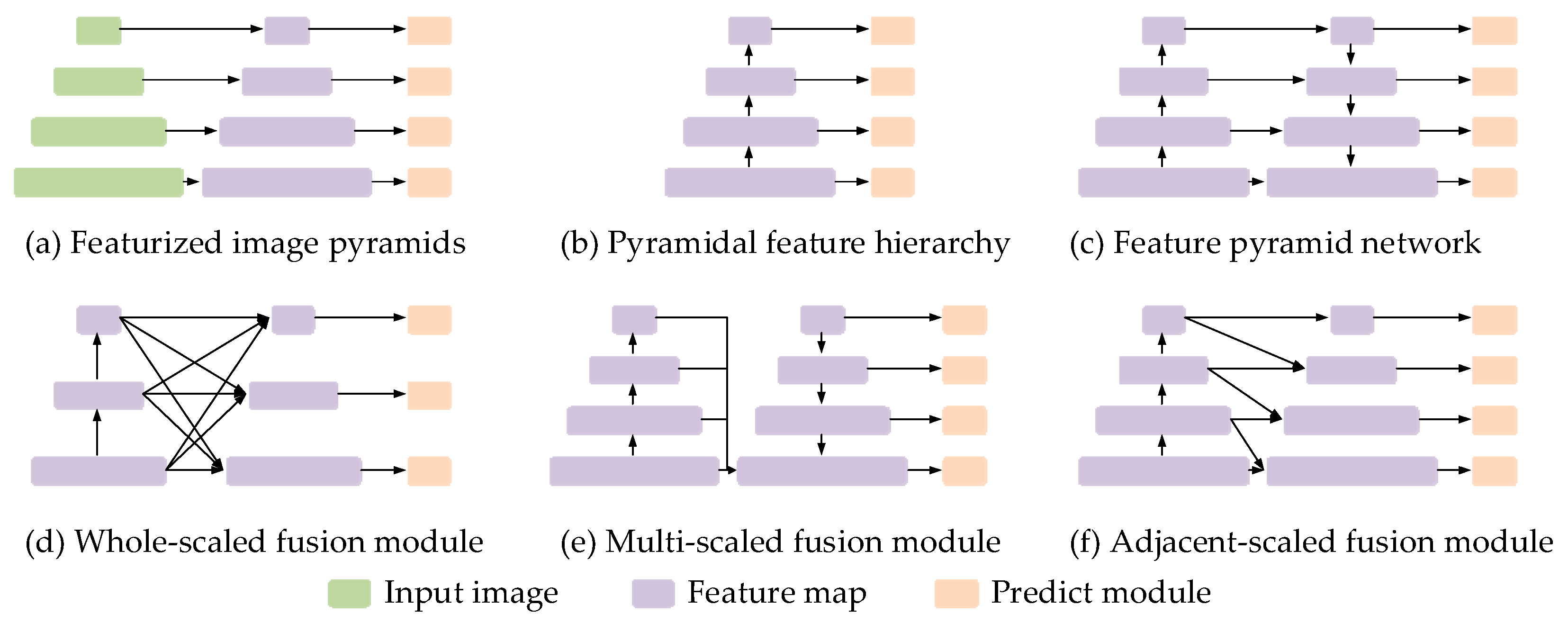
To alleviate this contradiction, multi-scale feature fusion methods have been explored. Existing research show that richer feature representations can be obtained by fusing features at different scales. As shown in Figure 1c–f, there are some typical feature fusion methods which have been proposed to obtain more discriminative representation on the base feature hierarchy. In addition to the feature fusion methods, the attention mechanism is also advantageous in feature selection and enhancement. By learning differentiated weights, important channels or areas of interest can be locally enhanced, which is beneficial for capturing features of small samples.

In this paper, we introduce two novel and effective blocks to enhance the original SSD, and propose a feature fusion and spatial attention-based single shot detector for small object detection, named FASSD. The main contributions of our works are summarized as follows:

(1) We propose a lightweight spatial attention block, which consists of continuous convolution, batch normalization, and activation function layers. It can learn an attention mask to enhance areas of interest and can be easily inserted into the network. Residual connection is adopted to prevent serious information loss after the attention mechanism.

(2) We present an effective feature fusion block that applies transposed convolution to upsample feature maps, and concatenation is adopted to fuse features. To adjust the number of channels, we utilize group convolution layers with 1 × 1 kernels.

(3) Applying the above two blocks, we design an improved framework based on SSD. Our FASSD achieves better performance on benchmark datasets of PASCAL VOC2007 than many improved frameworks based on SSD.

(4) We establish a Lake-Boat dataset for small object detection and prove the effectiveness of our algorithm. Our algorithm can detect surface objects with high accuracy and speed. This proves the high application potential of our work on water surface detection systems.

2. Related Work

Feature fusion methods and attention mechanisms have been widely applied in computer vision tasks for feature enhancement. In this section, we introduce related work from three aspects. We first summarize the application of feature fusion methods based on SSD. Then, we introduce recent developments in the attention mechanism. Finally, we present some common methods for small object detection.

2.1. Feature Fusion Methods Based on SSD

SSD is a multi-scale single shot detector that—inspired by the idea of image pyramids— creates feature pyramids for multi-scale object detection. After the backbone network, a fully convolutional network is added to extract a feature pyramid. However, SSD utilizes multi-layer features to perform detection independently, and effective information between different levels is not fully reused. In addition, the largest feature maps of 38 × 38 applied for small object detection do not contain sufficient semantic information, which limits the detection performance for small objects. Feature fusion is a common means of alleviating the contradiction between invariance and equivariance feature representations in a detection task [9]. Feature fusion methods can take charge of favorable information from different layers, such that location and semantic information can be integrated into one group of feature maps, while also importing contextual information at the same time. Therefore, the application of feature fusion methods to some algorithms has been proposed to enhance the feature extraction process.

2.1.1. Using a Feature Pyramid Network to Enhance Feature Extraction

In feature pyramid networks (FPNs) [6], as shown in Figure 1c, a top-down feature fusion architecture is designed with lateral connections. In this manner, a network of feature pyramids with high-level semantics at all scales is developed. By top-down enrichment, semantic gaps between different level feature maps can be narrowed observably, especially in deep ResNets. The same architecture is adopted by deconvolutional single shot detector (DSSD) [5], single shot refinement neural network (RefineDet) [10], and multi-level feature pyramid network based single shot detector (M2Det) [11]. DSSD uses deconvolution to upsample high-level features, and a skip connection is applied to transfer the corresponding low-level detail information to the layer after deconvolution. RefineDet inherits the advantages of the one-stage and two-stage detection strategies. The anchor refinement module filters out some negative anchors and roughly adjusts the object location. The object detection module then regresses the refined anchors further. RefineDet alleviates the imbalance problem of one-stage detectors. After fusing multi-scale features, M2Det designs a multilevel feature pyramid network (MLFPN) to construct more effective feature pyramids. Equivalent scale feature maps in MLFPN are integrated as hierarchical features.

2.1.2. Multi-Scale Feature Fusion

The feature fusion single shot multibox detector (FSSD) [12] uses multi-scale fusion feature maps to extract the feature pyramid. To induce multiple levels of feature information in the generated feature pyramid, FSSD first fuses multi-scale features, and then generates the feature pyramid from the fused feature maps. In this manner, multi-level location and semantic information is introduced into the generated feature pyramid. The rainbow single shot detector (RSSD) [8] proposes a connection method called rainbow concatenation, which realizes two-way information flow between low-level and high-level features. Interestingly, when performing unidirectional flow fusion, the detection performance deteriorates, and the detection speed decreases owing to the increase in computational complexity. The multi-scale deconvolutional single shot detector (MDSSD) [13] realizes the fusion of large-span feature maps; high-level features are fused with low-level features after multiple deconvolutions and convolutions, which improves the detection of small objects.

2.1.3. Enhanced Modules

To effectively combine fusion features, it is necessary to extract features by further convolution. CFENet [14] proposed a comprehensive feature enhancement (CFE) module to enhance features. The module is designed to enhance the shallow features for detecting small objects, which is actually motivated by the Inception module. The sizes of both the input and output feature maps of CFE are the same, such that they can be inserted wherever required. Receptive field block [15] aggregates multiple receptive fields (RFs) of various sizes and eccentricities. Different sizes of kernels and dilated convolution layers are assembled to provide various RFs with different eccentricities.

2.1.4. Dense Connection

Pre-training on ImageNet and then transferring the pre-trained models as network initialization parameters is widely adopted in the field of object detection. However, it is inappropriate in some cases, such as medical images, multispectral images, and synthetic aperture radar (SAR) images. Moreover, pre-training limits the flexible adjustment of the network structure. The deeply supervised object detector (DSOD) [16] uses DenseNet as the backbone network and uses dense connections to improve the structure of the prediction layers. These approaches realize a network model without pre-training.

The above feature fusion methods are beneficial for obtaining more discriminative feature representations, but the application scenarios are different. FPNs recover semantic information from the top layer, but information in the top layer is very limited. Generally speaking, FPNs can work better with ResNet. However, it brings an increase in calculation and decreases detection speed at the same time. The researcher needs to weigh according to the reality. In multi-scale feature fusion methods, directly fusing random layers will not work. The difficulty lies in the selection of fusion feature maps and fusion methods. Enhanced modules can be easily embedded into the network and enhance the feature extraction process, but where we put it and how many should we put needs to be verified through experiments. Dense connection retains all levels of feature maps, which is very beneficial for feature fusion. However, problems such as excessive GPU memory usage severely limit its application.

2.2. Attention Mechanism

The attention mechanism re-weights the original feature maps by modeling the dependencies between channels or pixels to filter or enhance the channels or areas of interest, which can effectively improve the quality of features and may benefit small object detection.

Channel attention focuses on the relationship between channels. The squeeze and excitation network (SENet) [17] uses the global pooling information of each channel to learn the relationship between channels, and uses compression and expansion methods to model channel relationships, thereby increasing the weight of important channels. Dynamic filter networks (DFN) [18] import information from the high stage to help learn the channel weight of the low stage.

Spatial attention focuses on the interrelationships of different areas. Residual Attention Network presents residual attention to learn a soft mask. The response of the background information can be better suppressed after the mask. Adaptively spatial feature fusion (ASFF) [7] utilizes spatial attention to optimize the feature fusion process. Non-local neural networks [19] capture long-range dependencies, which perform well in capturing contextual information.

In addition to independent use, the integration of channels and spatial attention has been attempted in many works. Global context network (GCNet) [20] combines a simplified non-local (NL) block and an SE module. The convolutional block attention module (CBAM) [21] learns channel and spatial attention weights from AvgPool and MaxPool values, and the two attention mechanisms are executed serially. Dual attention networks (DANet) [22] fuse dual attention results by element-wise sum to capture rich contextual dependencies for the scene segmentation task. Spatial and channel-wise attention in convolutional networks (SCA-CNN) [23] combine channel-wise attention and spatial attention on multi-layer feature maps to perform image captioning.

In the last three years, the attention mechanism has been widely used in computer vision to help improve the accuracy. But it is rarely applied to the related research of real-time detectors. Because the features of small objects are more sensitive to spatial dimension, the performance of spatial attention is stronger than channel attention. Therefore, our work only involves spatial attention.

2.3. Small Object Detection

2.3.1. Data Augmentation: Increasing the Number of Small Objects

Deep learning is driven by big data. In existing basic datasets, the rotation, cropping, or scaling of original images to increase the number of training samples has become a routine operation for improving the generalization ability and robustness of models. To solve the problem of the limited amount of small object samples in existing detection data sets, Kisantal et al. [24] adopted two methods: (1) oversampling and (2) pasting multiple segmentations of small objects into the original images. Such methods directly increase the proportion of small instances. It is simple but robust, and plays a role in balancing the number of positive and negative samples. However, the process is complicated and computationally demanding.

2.3.2. Detection in High-Resolution Maps

High resolution is beneficial for maintaining more spatial detail, which is significantly important for small object detection. However, with increasing hierarchy in ConvNets, the detailed information of small objects gradually diminishes. Some researchers utilize upsampling and super-resolution to obtain high-resolution maps. Chen et al. [25] added a separate context branch after the last convolution layer. The proposal regions were enlarged by 1.5 times before being sent to the prediction layer. Hu et al. [26] trained a multi-scale detector. When detecting small objects, the output feature maps from the last layer were first amplified through two times of interpolation. Li et al. [27] utilized a pre-trained perceptual GAN (generative adversarial network) to generate super-resolution feature representations of small objects. Perceptual GAN can improve the feature details of small objects to be comparable to those of large objects. Krishna et al. [28] took advantage of the convolutional–deconvolutional network introduced in the literature [29] for super-resolution expression of proposals. However, enlarging an image requires additional computing and storage resources, and super-resolution reconstruction networks often require separate training. Such training is not harmonious with the overall training process and decreases the detection speed.

2.3.3. Increasing the Number of Matching Anchors for Small Objects

To balance the number of large, medium, and small objects, on one hand, we can directly increase the number of small objects, such as with the data augmentation methods mentioned previously. On the other hand, increasing the number of matching anchors for small objects may be suitable. Setting smaller and denser anchors is a simple method. The single shot scale-invariant face detector (S3FD) [30] uses the equal-proportion interval principle to ensure that objects of different sizes can match the same number of anchors. At the same time, by setting a looser matching strategy for small objects (such as setting a lower IoU threshold for small objects), the number of matching anchors for small objects can also be increased [31].

3. Methods

In this section, we first describe the principle of the proposed FASSD and the two enhancement blocks: feature fusion block (FFB) and spatial attention block (SAB). Then, we discuss our training strategies. Finally, we introduce a new boat dataset for small object detection.

3.1. FASSD Architecture

Considering the difference in the distributions of object sizes in Visual Object Classes (VOC) and LAKE-BOAT, we applied different scale settings for the two datasets. Figure 2 and Figure 3 present the architecture of our FASSD and simplified FASSD with 300 × 300 input. VGG16 [32] is adopted as backbone network. Similar to DeepLab-LargeFOV [33], we convert fully connected layers (fc6 and fc7) to convolutional layers (conv6 and conv7). Fc8 layer and all dropout layers are removed. 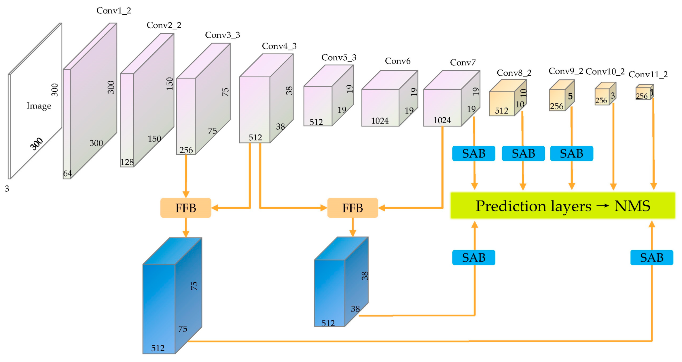Following the strategy in SSD [4], we add four convolutional layers to extract feature hierarchy. As shown in Figure 2, conv1 to conv7 are VGG16 layers, conv8 to conv11 are SSD layers.

3.1.1. FASSD Architecture

When performing multi-scale object detection, feature maps of different scales are responsible for responding to objects with corresponding scales, and the responses of small objects often occur in shallow layers. Considering the lack of semantic information in the shallow layers, we chose to import semantic information from adjacent scales up to the current layer, rather than recovering semantic information from the top layer. The feature maps at the top level are capable of extracting global semantics, but it is difficult to retain the local semantic information of small object areas. Multiple upsamplings may introduce noise, which will deteriorate the performance of small object detection.

To enhance the performance of small object detection, we added an extra scale of 75 × 75 compared with SSD. The feature maps of conv4_3 and conv7 were upsampled and concatenated with conv3_3 and conv4_3, respectively. The fused feature was integrated and extracted through further convolution in the feature fusion block. To ensure the versatility of FFB and reduce the design burden, the same FFBs were maintained except for the number of input channels and parameters of deconvolution layers. Spatial positions of interest were enhanced by inserting five spatial attention blocks into the network. Considering the lack of spatial information in the top two layers, they were not taken into consideration.

In the design of prediction layers, seven prediction layers were added to make prediction on seven-scale feature maps. For feature maps of size w × h with p channels, we applied 3 × 3 × p kernels to perform prediction at each of the w × h locations. Each prediction layer contained two convolutional layers which were applied to predict scores and location offsets respectively. The output channels were set to a × c and a × 4 where “a” represented the number of anchors about each cell of feature maps, “c” represented the number of object classes and “4” represented the number of location parameters. After prediction, NMS (non-maximum suppression) was applied to filter out redundant boxes during inference, targeting a final value of only 200 detections.

3.1.2. Simplified FASSD Version for Small Object Detection

Multi-scale detection is robust to scale variance. However, when the scale and size of the objects are similar, the great advantage of multi-scale detection is lost. Moreover, when small objects occupy a larger proportion of the dataset, the scale imbalance may prevent the training of high-level prediction layers, resulting in more false positives. To adopt the object characteristics of LAKE-BOAT, we directly removed high-level convolution layers after conv7, and only three scales were retained for prediction. Such an operation also reduces the inference time. The architecture of a simplified FASSD for small object detection is shown in Figure 3.

3.2. Feature Fusion Block

Two feature fusion blocks were used in our framework. Figure 4a shows their architectures. The dimension of all the feature maps was first reduced to 256 for computation optimization. To fit the special shape of feature maps from two layers, a deconvolution (transposed convolution) layer was added for upsampling. The kernel size was 3 × 3 or 2 × 2 with stride 2. We integrated the features through concatenation and further convolution. Every convolution or deconvolution layer was followed by ReLu layers. Batch normalization layers were extensively used to prevent feature divergence.

To optimize the computation, we applied four 1 × 1 convolution layers for dimensionality adjustment. We utilized two 1 × 1 convolution layers to reduce the channels of input feature maps to 256 each before concatenation. Before and after further convolution, a 1 × 1 convolution layer was used to reduce or restore the channels. Specifically, all 1 × 1 convolutional layers adopt the form of group convolution, which is inspired by ResNext [34]. All the parameters of the groups were set to 32. In ordinary convolution, each output channel is connected to all input channels. Group convolution divides the input and output channels into multiple groups, and each group follows the ordinary convolution operation, but there is no information interaction between groups. Therefore, group convolution is more conducive to retain the differences between channels.

3.3. Spatial Attention Block

Small objects merely occupy a small area. We attempted to design a lightweight block to enhance the possible regions of small objects while suppressing the background response at the same time. To this end, we designed a spatial attention block consisting of continuous convolution, batch normalization, and activation function layers. To prevent serious information loss after attention, we utilized leaky ReLu instead of ReLu and also adopted the residual connection. SAB can learn an attention mask to enhance the area of interest. Element-wise products were applied to fuse the mask with each channel of the feature maps. Our structure is completely differentiable, and the parameters can be updated well in back-propagation.

We designed two versions of the spatial attention block, as shown in Figure 4. One possesses only a single branch, as shown in Figure 4b, and only 1 × 1 convolution is utilized for channel integration. It performs computations only at a certain position between different channels, without changing the receptive fields of the previous feature maps. The other possesses two branches, as shown in Figure 4c. We introduced dilated convolution to improve the contextual information awareness of our attention blocks.

Assuming that the original feature maps are x, the new feature maps after attention are y and express the attention operation of each branch as function F. Thus, the attention mechanism can be expressed as follows (taking the version with two branches as an example):

$$\begin{gathered} \alpha =F_{\alpha }(x) \\ \beta =F_{\beta }(x) \\ y=(\alpha +\beta +1)x=(\alpha +\beta )x+x \end{gathered}$$

(1)

$\alpha$ and $\beta$ represent the attention mask learned by two of the branches.

3.4. LAKE-BOAT Dataset for Small Object Detection

Small object detection has a greater demand for context information. To evaluate our framework more accurately, we constructed a LAKE-BOAT dataset under a typical lake scene. The lake scene we constructed has obvious background information on the water surface, which can effectively test the capability of the detection model for extracting context information.

The LAKE-BOAT dataset contained 350 images, in which 250 images were taken for training and the remaining 100 images were taken for testing. The original image size was 960 × 540 pixels. To increase the number of small instances, we performed a sample offline data augmentation by zooming out the original images. We first reduced the original width and height by half and then spliced it to four segments to restore the original resolution, as shown in Figure 5. Label files were used to perform the corresponding conversion. The orange bounding boxes illustrate annotation results.

We analyzed the size attribute of objects’ ground truth box after resizing the image to 300 × 300, and the results are shown in

Table 1. Size attribute of objects in LAKE-BOAT.

	Train Set	Aug Set	Training Set	Test Set
Images	250	250	500	100
Objects	954	3816	4770	625
Extra-small objects	465	3084	3549	426
Small objects	314	580	894	134
Medium objects	138	132	270	48
Large objects	32	20	52	13
Extra-large objects	5	0	5	4
Proportion of extra-small and small objects	81.7%	96.0%	93.1%	89.6%

. Small objects and extra-small objects accounted for an extremely large proportion. Extra-small objects, small objects, medium objects, large objects, and extra-large objects correspond to levels 1 to 5, respectively. The area corresponding to level x is calculated according to Formula (2), and the corresponding size in the 300 × 300 images and 75 × 75 feature maps are shown in

Table 2. Correspondence size in 300 × 300 images and 75 × 75 feature maps of objects.

Level	Attribute	75 × 75 maps	300 × 300 Images
1	Extra-small	0–32	0–122
2	Small	32–62	122–242
3	Medium	62–122	242–482
4	Large	122–242	482–962
5	Extra-large	242–	962–

.

$$\{\begin{array}{l}x=1 0<\mathrm{s}\le {(12\times 2^{x-1})}^2\\ x=2,3,4 (12\times 2^{x-2}{)}^2<\mathrm{s}\le (12\times 2^{x-1}{)}^2\\ x=5 \mathrm{s}>(12\times 2^{x-2}{)}^2\end{array}$$

(2)

3.5. Training

3.5.1. Data Augmentation

We adopted the same online strategies for SSD. In addition, we applied a simple offline augmentation method (Section 3.4) to train our model on the LAKE-BOAT dataset. In this manner, we obtained a new dataset with four-times-smaller objects. The original dataset and the augmented version were combined for further training.

3.5.2. Transfer Learning

Transfer learning can effectively improve the robustness of the model and speed up convergence. For the VOC task, we used the pre-trained VGG16 [32] on the ILSVRC CLS-LOC dataset as initial weights. When training on the LAKE-BOAT dataset, we transferred the corresponding parameters from well-trained FASSD on VOC, except for the prediction layers. After transferring the weights, we first trained the prediction layer separately and then fine-tuned the network.

3.5.3. Anchor Setting

For the VOC task, the same setting strategy as the corresponding SSD level was adopted for the last six prediction layers. The scale of conv4_3 was 0.2, and the scale of the top layer was 0.9. As for the extra level, we set a smaller scale of 0.1. For conv7, conv8_2, conv9_2, six anchors were set for ratios $\left\{1, 2, 3, \frac{1}{2}, \frac{1}{3}\right\}$ in each cell of the feature maps. The other convolutions included four anchors in ratios $\left\{1, 2, \frac{1}{2}\right\}$. For the LAKE-BOAT task, the anchor setting of the remaining three scales applied the same strategy.

3.5.4. Loss Function

Following in SSD’s footsteps, we utilized Smooth L1 loss and Softmax loss to measure the localization loss and confidence loss respectively. The model loss is a sum of localization loss and confidence loss.

Our training strategies follow the baseline network. Some common points are not mentioned. Interested readers can refer to the original paper [4] for more details.

4. Experiments

For our experiments, the Pytorch-version SSD provided by [35] was selected as the baseline. We evaluated our FASSD on PASCAL VOC and LAKE-BOAT. PASCAL VOC is one of the most common benchmark datasets in object detection. It provides labeled images and evaluation toolbox of precision for researchers. The PASCAL VOC dataset contains 20 types of objects, including person, cat, bus, bottle, etc. VOC2007 annotated 9963 images and 24,640 objects in which 4952 images and 12,032 objects are taking for test; the trainval set of VOC2012 annotated 11,530 images and 27,450 objects. We adopt the common index mAP (mean average precision) and FPS (frame per second) to evaluate the detection accuracy and speed. The mAP is calculated by the official devkit provided by PASCAL VOC.

4.1. Ablation Study of VOC

To compare the contribution of each improvement measure, we performed our experiments on VOC with an input size of 300 × 300. All models were trained on the union of the 2007 and 2012 trainval (VOC07 + 12) and tested on the VOC2007 test set. The results are shown in

Table 3. Results of the ablation study on PASCAL VOC2007.

Method	75 × 75	Attention		Fusion	Anchors	mAP	FPS
		v1	v2
SSD300	✘	✘	✘	✘	8732	77.7	69.7
FASSD300	✘	✔	✘	✘	8732	78.1	67.8
FASSD300	✘	✘	✔	✘	8732	78.0	58.4
FASSD300	✘	✘	✔	✔	8732	78.2	47.8
FASSD300	✔	✘	✘	✔	31,232	78.2	54.2
FASSD300	✔	✔	✘	✔	31,232	78.9	52.4
FASSD300	✔	✘	✔	✔	31,232	79.3	45.3

. All the results were tested by ourselves using a signal TITAN RTX GPU, an Intel I9-10900X@3.70GHz, and cuda 10.1, pytorch 1.0.0. We used 500 images from the VOC2007 test and resized them to 300 × 300 before the speed test. A value of 75 × 75 indicates whether to add the extra scale feature maps of 75 × 75 for detection.

4.1.1. Extra Scale of 75 × 75

The extra scale with small anchors is important for detecting small objects. In Table 3, we compare the versions of models that apply attention v2 and feature fusion (row 4), and extra scale and attention v2 and feature fusion (row 7). The results indicate that an extra scale can increase the mAP by 1.1%. However, utilizing the extra scale and feature fusion method (row 5) only increases the mAP by 0.5%, which indicates that it works best when applying the three methods simultaneously.

4.1.2. Feature Fusion

In Table 3, we compare the versions of models that apply attention v2 (row 3) and attention v2 and feature fusion (row 4). The results indicate that feature fusion methods can increase the mAP by 0.2%, while the increase in computation decreases the detection speed by 18%. The results also indicate that simple fusion does not necessarily bring considerable performance improvements. The choice of fusion feature maps is crucial.

4.1.3. Two Versions of SAB

We performed two groups of contrast to compare the performance of SAB v1 and SAB v2. By directly adding four SABs before the head of SSD, the two versions of SAB both achieved an improvement of 0.4% and 0.3% mAP. However, the performance of SAB v2 was lower than that of SAB v1. On the contrary, mAP slightly decreased. The result in the second row of Table 3 shows that SAB v1 is a lightweight plug-and-play block. With the extra scale of 75 × 75 and application of feature fusion, SAB v2 achieved a better grade than SAB v1 at about 0.4% mAP. The results indicate that dilated convolution is more suitable for capturing detailed information, especially in large-scale feature maps.

4.1.4. Group Convolution

A 1 × 1 convolution layer is often used as a bottleneck layer for dimensionality reduction. As in our attempt in the attention block, a 1 × 1 convolution layer can also integrate features from multiple channels but it is not beneficial for further fusion and extraction. After 1 × 1 convolution, the difference between channels decreased, which further deteriorated the learning process. Therefore, we replaced the general convolution layers with the group convolution layers in the FFB. This operation increased the mAP from 78.7% to 79.3%.

4.2. Results on PASCAL VOC2007

We trained our FASSD on the union of the VOC2007 trainval and VOC2012 trainval, and tested it on VOC2007. Following the SSD, we set the batch size to 32 with the input 300 × 300 and trained FASSD for 120,000 iterations. The learning rate was set to 10⁻³ for the first 80,000 iterations, and then adjusted to 10⁻⁴ and 10⁻⁵ for the next and last 20,000 iterations, respectively. The SGD optimizer with a momentum of 0.9 and a weight decay of 0.0005 was adopted. The initialization parameters of the backbone were derived from a well pre-trained VGG16 on ImageNet, and Xavier initialization was applied to the remaining layers.

The results of the PASCAL VOC2007 test are shown in

Table 4. Results on PASCAL VOC2007 test.

Method	Backbone	mAP	Aero	Bike	Bird	Boat	Bottle	Bus	Car	Cat	Chair	Cow	Table	Dog	Horse	mBike	Person	Plant	Sheep	Sofa	Train	TV
Faster [36]	VGG	73.2	76.5	79.0	70.9	65.5	52.1	83.1	84.7	86.4	52.0	81.9	65.7	84.8	84.6	77.5	76.7	38.8	73.6	73.9	83.0	72.6
Faster [37]	Residual-101	76.4	79.8	80.7	76.2	68.3	55.9	85.1	85.3	89.8	56.7	87.8	69.4	88.3	88.9	80.9	78.4	41.7	78.6	79.8	85.3	72.0
CSSD300 [38]	VGG	78.1	82.2	85.4	76.5	69.8	51.1	86.4	86.4	88.0	61.6	82.7	76.4	86.5	87.9	85.7	78.8	54.2	76.9	77.6	88.9	78.2
DSSD321 [5]	Residual-101	78.6	81.9	84.9	80.5	68.4	53.9	85.6	86.2	88.9	61.1	83.5	78.7	86.7	88.7	86.7	79.7	51.7	78.0	80.9	87.2	79.4
MDSSD300 [13]	VGG	78.6	86.5	87.6	78.9	70.6	55.0	86.9	87.0	88.1	58.5	84.8	73.4	84.8	89.2	88.1	78.0	52.3	78.6	74.5	86.8	80.7
SSD300* [4]	VGG	77.5	79.5	83.9	76.0	69.6	50.5	87.0	85.7	88.1	60.3	81.5	77.0	86.1	87.5	84.0	79.4	52.3	77.9	79.5	87.6	76.8
SSD512* [4]	VGG	79.5	84.8	85.1	81.5	73.0	57.8	87.8	88.3	87.4	63.5	85.4	73.2	86.2	86.7	83.9	82.5	55.6	81.7	79.0	86.6	80.0
SSD300	VGG	77.7	82.5	83.5	75.9	70.8	49.5	85.4	86.4	88.7	61.2	82.0	78.9	85.3	86.8	84.7	79.3	54.0	75.3	79.1	86.8	78.3
FASSD300	VGG	79.3	86.2	84.8	77.1	75.8	54.1	85.7	87.5	89.1	61.7	85.4	77.2	86.6	88.7	86.4	79.9	54.4	79.5	80.4	88.4	76.2

SSD300 is the Pytorch version, which was trained and tested by ourselves. SSD300* and SSD512* are updated Caffe versions of the new expansion data augmentation trick.

. By utilizing powerful data augmentation methods, the Pytorch-version SSD trained by ourselves beyond the latest Caffe version by 0.2 points, proposed by the authors after the paper publication. Our FASSD achieved 79.3% mAP with an input of 300 × 300, outperforming the baseline by 1.6 points with a similar performance to that of SSD512*. FASSD also outperformed CSSD, DSSD, DSOD, MDSSD, RSSD, and FSSD with similar input sizes.

4.3. Inference Speed on PASCAL VOC2007 Test

Table 5. Comparison of speed and accuracy on the PASCAL VOC2007 test.

Method	Backbone	mAP	FPS	# Proposals	GPU	Input Size
Faster [36]	VGG	73.2	7	6000	Titan X	~1000 × 600
Faster [37]	Residual-101	76.4	2.4	300	K40	~1000 × 600
CSSD300 [38]	VGG	78.1	40.8	-	Titan X	300 × 300
DSSD321 [5]	Residual-101	78.6	9.5	17,080	Titan X	321 × 321
DSOD [16]	DS/64-192-48-1	77.7	17.4	-	Titan X	300 × 300
FSSD300 [12]	VGG	78.8	65.8	8732	1080Ti	300 × 300
MDSSD300 [13]	VGG	78.6	38.5	31,232	1080Ti	300 × 300
RSSD300 [8]	VGG	78.5	35	8732	Titan X	300 × 300
SSD300* [4]	VGG	77.5	46	8732	Titan X	300 × 300
SSD512* [4]	VGG	79.5	19	24,564	Titan X	512 × 512
SSD300	VGG	77.7	69.7	8732	TITAN RTX	300 × 300
FASSD300	VGG	79.3	45.3	31,232	TITAN RTX	300 × 300

shows the inference speed of Faster R-CNN and some networks based on SSD. Our FASSD can run at 45.3 FPS with an input size of 300 × 300 on a signal TITAN RTX GPU. For fair comparison, we tested the speed of SSD with the same settings. Because of the additional layers, our FASSD is 35% slower than SSD. However, compared with DSSD, MDSSD, and DSOD, our framework is very competitive with better performance in terms of both speed and accuracy.

4.4. Small Object Detection on LAKE-BOAT

To further evaluate the performance of our model, we designed experiments using the LAKE-BOAT dataset. For better convergence and faster training, we transferred the corresponding parameters from the corresponding version trained on the VOC model. Taking the number of images into consideration, we trained our model on LAKE-BOAT for only 7000 iterations. The learning rate was set to 10⁻³ for the first 1000 iterations, and then decreased to 10⁻⁴ for the next 4000 iterations, 10⁻⁵ for another 1000 iterations, and 10⁻⁶ for the last 1000 iterations. In the first 1000 iterations, we froze all parameters except for the prediction layers, after which we fine-tuned the entire network.

4.4.1. Results and Inference Speed

SSD300 maintains the same architecture as the VOC task, except for the prediction kernels. For a fair comparison, we trained a simplified version of SSD. SSD300^# removed the extra layers after conv7, and the feature maps from conv3_3 were used for prediction. The inference time was tested using a signal TITAN RTX GPU, an Intel I9-10900X@3.70GHz, and cuda 10.1, pytorch 1.0.0. We used 100 images of the Lake-Boat test and resized them to 300 × 300 before testing. The comparison results are shown in

Table 6. Results and inference speed with LAKE-BOAT.

Method	mAP	FPS
SSD300	67.3	67.6
SSD300#	71.8	86.6
FASSDv1	75.3	64.4
FASSDv2	74.1	57.8

.

By simplifying the architecture, the network can adapt to the target scene better, which significantly improves the detection speed. The simplified version of the SSD can run at 86.6 FPS. Because of the complexity of the scene and the objects’ dense distribution, the original version of SSD runs slightly slower than the test on the VOC dataset. Our FASSDv1 achieved a mAP of 75.3% while maintaining a real-time detection speed of 64.4 FPS, which exceeds the original version of SSD by 8 points and outperforms the simplified version of SSD by 3.5 points. The results indicate that our feature fusion block and spatial attention block perform well in enhancing the shallow layers. Contrary to the previous results on VOC, our model utilizing SAB v1 performs better than SAB v2. This phenomenon is closely related to the object size. In theory, the receptive field shared by SAB v2 is 125 times larger than SAB v1. Because some of the boat instances are extremely small, excessive background information will be imported when SAB v2 is applied.

4.4.2. Transfer Learning and Data Augmentation

We conducted a simple ablation study to evaluate the contribution of transfer learning and offline data augmentation. The comparison results are shown in

Table 7. Results of the ablation study on LAKE-BOAT.

Method	Transfer Learning	Data Augmentation	mAP
FASSD300	✔	✔	75.3
FASSD300	✔	✘	73.9
FASSD300	✘	✔	71.1

.

When pre-training was applied, the same strategy as in Section 4.3 was maintained for the setting of the learning rate. However, it was difficult to train our model using a large learning rate. Loss value explosion invariably occurred without parameter transfer, which hindered the training process. Moreover, 7000 iterations are not sufficient to train the model well. Therefore, the initial learning rate was changed to 10⁻⁴ for the first 20,000 iterations. Then, we decrease it to 10⁻⁵ and 10⁻⁶ for the next 10,000 iterations and last 10,000 iterations.

The results indicate that transfer learning is beneficial for the training process, especially for a small dataset. Transfer learning increased mAP by approximately 4.2 points. Data augmentation contributed to mAP by 1.4 points. This result suggests that the simultaneous use of online and offline data augmentation methods is beneficial when dataset is small.

4.4.3. Detection Rate and False Alarm Rate

In practical applications, the number of detected objects and false predictions are often of research interest. Considering this, we define the detection rate (DR) as the proportion of detected objects to the number of real objects, and the false alarm rate (FAR) as the proportion of false predictions to all predictions. The correctness of a prediction is determined by the intersection over union (IoU) of the prediction and the truths. IOU > 0.5, or not, is the judgment standard. False predictions include incorrect classification and poor position regression. DR and FAR can help evaluate the performance of the models more scientifically. By setting different confidence thresholds, we obtained corresponding results of DR and FAR. The analysis results of DR with FAR of 5%, 10%, and 20% are shown in

Table 8. Detection rate when false alarm rate is 0.05, 0.10, or 0.20.

FAR	Method	E-Small	Small	Medium	Large	E-Large	All
0.05	SSD300	0.178	0.910	0.979	1	1	0.419
	SSD300#	0.244	0.970	0.979	1	1	0.477
	FASSDv1	0.378	0.978	0.979	1	1	0.570
	FASSDv2	0.380	0.978	0.979	1	1	0.571
0.10	SSD300	0.289	0.955	0.979	1	1	0.504
	SSD300#	0.430	0.978	0.979	1	1	0.605
	FASSDv1	0.521	0.978	0.979	1	1	0.667
	FASSDv2	0.486	0.978	0.979	1	1	0.643
0.20	SSD300	0.418	0.970	0.979	1	1	0.595
	SSD300#	0.538	0.985	0.979	1	1	0.680
	FASSDv1	0.608	0.978	0.979	1	1	0.726
	FASSDv2	0.592	0.978	0.979	1	1	0.715

The ground truth boxes’ size of extra-small, small, medium, large and extra-large objects are 0–12², 12²–24², 24²–48², 48²–96², and 96²– pixels after resize to 300 × 300 according to Table 2.

, and the relationship between DR and FAR is shown in Figure 6.

As shown in Table 8, all four models performed well in the detection of medium, large, and extra-large objects, with only few difficult instances being missed. However, our model significantly outperformed the original and simplified version of SSD in the detection of extra-small objects. FASSDv1 outperformed the simplified version of SSD by 13.6%, 9.1%, and 7% at FAR of 5%, 10%, and 20%, respectively.

4.5. Visualization Analysis

Figure 7 shows the visualization of feature maps. Through the attention mechanism, the area of the objects was enhanced. The contrast between the area of interest and the background was significantly improved. In the first and second rows, background information could be balanced and suppressed. For small objects in the third and fourth rows, the spatial attention block highlighted the center of objects and distinguished boundary information.

4.6. Visualization of Results

Figure 8 shows the results of detection for the PASCAL VOC2007 test. The confidence threshold was set to 0.6. Compared with the conventional SSD, our model showed performance improvements from three aspects. The first is in terms of small object detection, as shown in Figure 8a. Owing to the shortage of semantic information in shallow layers and the small size of feature maps, SSD could not perform well, but our model showed targeted improvement. The second is in terms of dense and occluded cases, as shown in Figure 8b. This improvement may be attributable to the spatial attention block, which can effectively enhance the contrast between objects and the background. The third is for objects with rich contextual information, as shown in Figure 8c. Our FASSD takes contextual information into account and avoids mistaking the sheep in the flock for cows.

Figure 9 shows the results of detection with the LAKE-BOAT dataset. Only the predictions with confidence scores higher than 0.15 are displayed. We show the comparison of the simplified SSD and FASSDv1. Figure 9a indicates our model’s advantage in small object detection. As shown in Figure 9b, our model is more robust in the occluded and dense cases. Figure 9c shows that our model works better in capturing contextual information. Without enhancement in shallow layers, the simplified SSD generated some false predictions.

5. Conclusions and Future Work

In this paper, we proposed an effective feature fusion block and a lightweight spatial attention block to enhance the sematic information of the shallow layers. The feature fusion blocks fuse sematic information from an adjacent scale. The spatial attention blocks utilize continuous convolution, batch normalization, and activation function layers to learn the special attention weights. On the basis of the two blocks, we propose a feature fusion and spatial attention-based single shot detector. Our FASSD achieves higher performance than many existing detectors with benchmark datasets while still maintaining a real-time detection speed. Experiments conducted with LAKE-BOAT demonstrate the capability of our model in small object detection.

In our model, we utilized an input of 300 × 300 for real-time detection. However, it could not fully utilize all the information of the original 960 × 540 images. The precision may be improved by increasing the input size, but the simultaneous optimization of inference time remains to be addressed, which is the focus of our future work. Our spatial attention block is lightweight and can conveniently be inserted into any ConvNets. It can be applied to other computer vision tasks that are sensitive to spatial information, such as segmentation tasks. The branch with 1 × k or k × 1 kernels can be used to capture horizontal or vertical connections in pedestrian detection. We will investigate these issues in our future work.