Optimization of Spiking Neural Networks Based on Binary Streamed Rate Coding

Abstract

Spiking neural networks (SNN) increasingly attract attention for their similarity to the biological neural system. Hardware implementation of spiking neural networks, however, remains a great challenge due to their excessive complexity and circuit size. This work introduces a novel optimization method for hardware friendly SNN architecture based on a modified rate coding scheme called Binary Streamed Rate Coding (BSRC). BSRC combines the features of both rate and temporal coding. In addition, by employing a built-in randomizer, the BSRC SNN model provides a higher accuracy and faster training. We also present SNN optimization methods including structure optimization and weight quantization. Extensive evaluations with MNIST SNNs demonstrate that the structure optimization of SNN (81-30-20-10) provides 183.19 times reduction in hardware compared with SNN (784-800-10), while providing an accuracy of 95.25%, a small loss compared with 98.89% and 98.93% reported in the previous works. Our weight quantization reduces 32-bit weights to 4-bit integers leading to further hardware reduction of 4 times with only 0.56% accuracy loss. Overall, the SNN model (81-30-20-10) optimized by our method shrinks the SNN’s circuit area from 3089.49 ${\mathrm{mm}}^2$ for SNN (784-800-10) to 4.04 ${\mathrm{mm}}^2$—a reduction of 765 times.

1. Introduction

In recent years, various types of Artificial Neural Network (ANN) have been studied as effective solutions for many object recognition and image classification problems with increasing accuracy. The Modified National Institute of Standards and Technology (MNIST) dataset is one of the popular benchmarks for testing different types of ANN due to its simplicity. MNIST dataset contains 60,000 and 10,000 images of handwritten digits for training and testing neural network modules, respectively. Training and evaluating various types of ANNs on large datasets consume a lot of time. Furthermore, while keeping a high level of accuracy, designing an ANN of minimal model size or hardware cost is even more challenging. There is a growing demand for hardware-friendly ANN optimization due to the rapid growth in low power AI for IOT and edge AI accelerator technologies. Among the ANN models, SNN is receiving growing attention due to its structural resemblance to the biological neural system. In addition, SNN is known to require less hardware leading to smaller chip size and lower power consumption [1,2]. Many hardware accelerators have been reported for SNN, which include SpiNNaker/SpiNNaker-2 [3,4], Intel Loihi [5] and Neurogrid [6], and TrueNorth chip [7]. In this paper, we present a highly optimized SNN with relatively high accuracy aimed at a compact SNN hardware accelerator. We propose a novel spiking signal coding scheme, and present SNN model optimization and quantization techniques, which are summarized as follows.

First, we propose a new rate-based spike generation method called a Binary Streamed Rate Coding (BSRC), which allows easy implementation in both software and hardware. BSRC eliminates the need for adding random noise to the input image pixels like traditional rate coding [8,9,10]. Instead, we can directly generate spike signals corresponding to all pixels of the entire input image. Second, we introduce a training technique for the proposed SNN. Recently, a direct supervised training algorithm for SNN called STBP was published [11]. It can reportedly achieve a very high accuracy of 99.42% using the MNIST dataset. We show in the experimental section that our BSRC coding scheme method, when combined with STBP, provides even higher accuracy.

It is a great challenge to design hardware accelerators of an SNN for low power and compact embedded devices. This is especially the case because hardware resources like memory, multipliers, and adders are limited. The accelerator designs are also constrained by the size of the ANN model, design complexity, operation speed, and power consumption [12,13,14,15,16,17]. In [18], the authors discussed an efficient technique for reducing the number of bits in representing SNN weights for training and inference process using either fixed-point or floating-point calculations. The authors in [19] further reduced the number of required weight bits into two bits for the inference process using an ANN training algorithm called BinaryConnect [20]. Then, they converted the ANN model to an SNN model and reported an accuracy of 99.43% on MNIST dataset. In [21], the authors reported an energy-efficient convolutional SNN by converting a deep CNN into an SNN to implement it to a spike-based neuromorphic hardware. In [14], a hybrid updating algorithm was proposed, which combines the advantages of existing algorithms to reduce the hardware complexity and improve the system performance. They proposed a network module supporting up to 16,384 neurons with a total of 16.8 million synapses. The design of [14] reported a reduced power consumption of 0.477 W, while achieving a relatively high accuracy of 97.06% for the MNIST dataset.

Many research studies on SNN have gradually improved the accuracy of the MNIST dataset. SNNs can be grouped to two types: fully connected SNNs [1,22] and convolutional SNNs [18,19]. Fully connected (FC) network is our choice, because of its simplicity for hardware implementation. In the fully connected networks, all neurons in one layer are connected to every neuron in the next layer. The nature of nondifferentiable spiking function and the dynamic feature make the training process of SNN incredibly challenging. Training an SNN can be done in three different methods:

• Unsupervised training is a kind of self-training for synapse weight modification inspired by biological neural system exhibiting spike timing dependence plasticity [23,24,25].
• Indirect supervised training is a method that first trains the network model as an ANN through using traditional training algorithms, and then converts the trained network model into SNN version [26,27,28].
• Direct supervised training is a method that attempts to train an SNN directly by using approximated version of spiking function [11]. These training algorithms should have the capability to utilize spatial domain property to increase the training accuracy [22].

The proposed work introduces a new type of direct supervised training method based on Binary Streamed Rate Coding (BSRC). We then efficiently combine the time and spatial domain information to obtain higher accuracy than other algorithms.

2. Structure of Spiking Neural Network

2.1. Overall Structure of SNN

Spiking neural networks commonly consist of spiking neurons, synapses, and interconnections between neurons and synapses. Synapses are often modeled by adjustable weights. A type of SNNs comprises only fully connected layer(s), while other types comprise convolutional layer(s) as well as fully connect layer(s). In the fully connected type of SNNs, all neurons in the preceding layer are fully connected to every neuron in the subsequent layer [26]. Figure 1a shows the general structure of a fully connected SNN for 28 × 28 MNIST dataset. The training or inference processes start by flatten the input image pixels from two-dimensional array of 28 × 28 to a one-dimensional vector of size 784. After the input image flattening, the input layer of the network converts each input pixel’s integer value to spike signals using various methods such as temporal coding and rate coding. The output layer consists of neurons, whose outputs represent the classes of MNIST.

For low cost hardware implementation, the full-scale input image can be scaled down to reduce the SNN size. For example, Figure 1b shows a reduced SNN that takes as input the MNIST images scaled downed to 9 × 9.

The full scale SNNs and reduced SNNs have been used to evaluate our proposed SNN optimization and quantization methods.

Through an extensive analysis of performance-to-cost metric, we chose an SNN structure consisting of two fully connect hidden layers with various image size (28 × 28, 14 × 14, 9 × 9) and various number of neurons in each layer. Our SNN model represents each pixel integer value in a binary stream of spikes using the proposed rate coding scheme called a Binary Streamed Rate Coding (BSRC). Like other SNN models, our SNN model also distinguishes between two types of synapses, excitatory and inhibitory synapses, which are denoted by red and blue colors, respectively, in Figure 1a,b.

Throughout our paper, we define an SNN’s dimension by a list of each layer’s size (the number of neurons). For example, (784-800-10) represents an SNN consisting of the input layer with 784 neurons, first hidden layer with 800 neurons, and the output layer with 10 neurons.

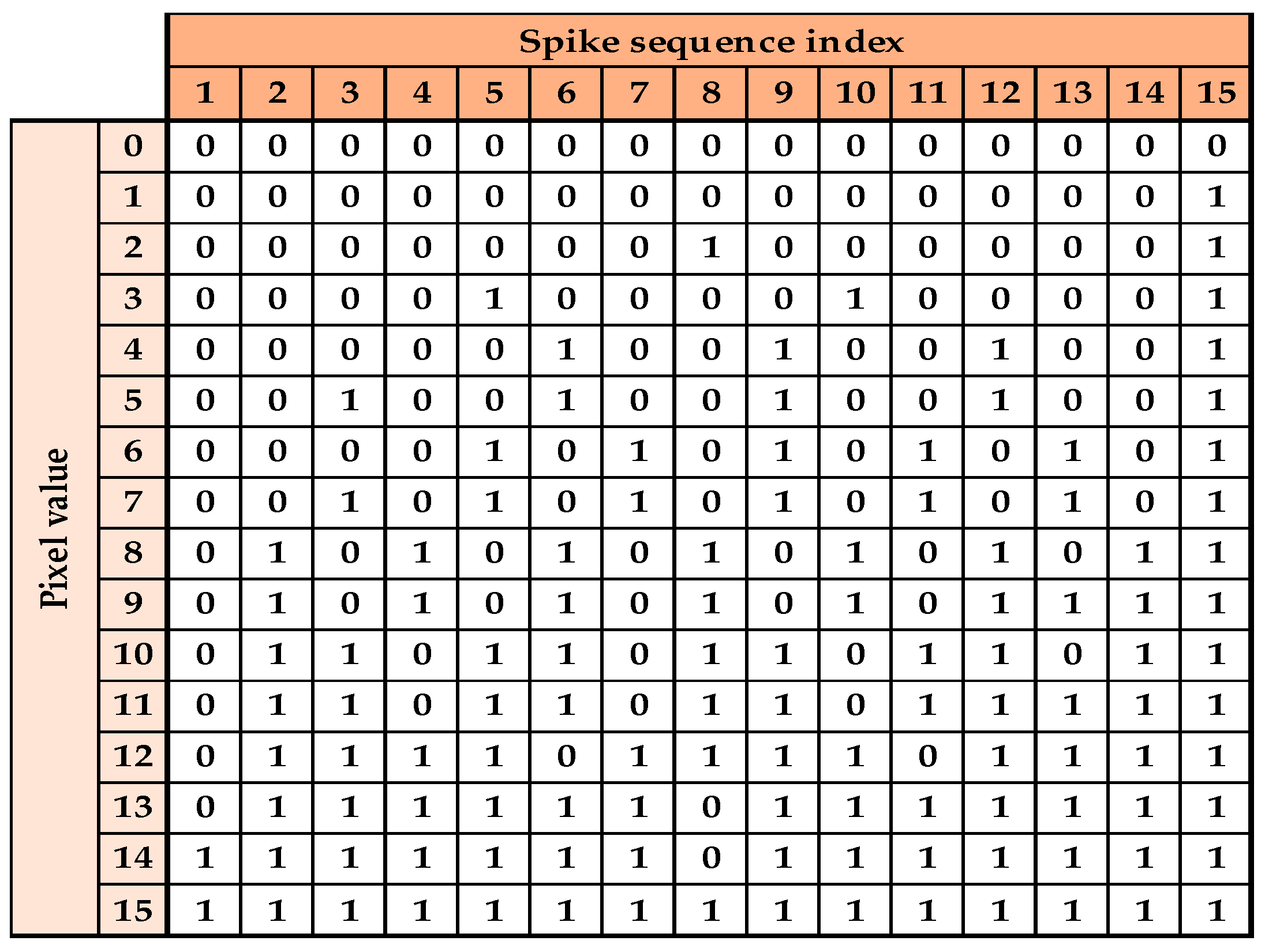
2.2. Spike Signal Representation

Spiking neural networks are more plausible than other types of biological neuron ensembles. Most of SNNs process spike signals in two domains (temporal and spatial) [11], which provides prominent advantage over traditional ANNs which have only spatial domain. Figure 2 illustrates the differences between ANN and SNN’s neuron models. Note the differences in the input signal, multiplication and addition processes, activation function, and the output signal.

Coding schemes play an important role in representing the spike signals in each layer and training the SNN with the temporal and spatial domains. There are two common coding schemes for converting input pixel value in SNNs: rate coding and temporal coding [10,11]. The rate-based coding scheme is regarded as highly demanding for training and implementation, since it results in a large number of weight lookups and high spike traffic in the routing fabric [29]. Another difficulty is that high spike rate tends to mask the discrete nature of the spiking activity [30], On the other hand, the temporal coding SNNs tend to suffer from poor accuracy. For example, in [29,30], where temporal based coding was used, the authors reported low accuracies of 96.8% and 97.55% respectively, for the SNN of size (78-4800-10). In our work, we developed a hardware-friendly rate coding SNN model called Binary Streamed Rate Coding (BSRC) which can overcome the above drawbacks.

BSRC converts the input pixel values to rate-based spike signals represented by a binary stream. The length T of spike streams is determined with consideration of the hardware implementation cost. We represent each spike signal in each layer of SNN by a stream of T binary values with 1 indicating the presence of a spike and 0 indicating no spike. Each image in the MNIST dataset consists of pixels represented in integer values like most image data. In the proposed method, Algorithm 1 converts each input pixel’s integer value to a stream of binary values representing the rate of spikes in the pre-determined stream length T. For a pixel value of n-bits, the pixel is converted to a sequence of 2ⁿ− 1 bits. Hence, the sequence length $T$ is given by Equation (1):

$$T =(2^n-1)$$

(1)

Line 2 and 6 of Algorithm 1 separate the pixel values into two groups. The pixel value Pv satisfying the condition $0 < Pv < int\left(T/2\right)$ falls into the first group (line 2). For the first group, line 4 of Algorithm 1 sets the bits to ones that correspond to spike positions. On the other hand, the pixel values Pv meeting $int(T$/2) $\le$ Pv falls into the second group (line 6). For the second group, line 7 of Algorithm 1 initializes the spike stream S_spikes by all ones and sets the bits to zeros that correspond to non-spike positions (line 14). As the final step in each group, the stream of spikes is rotated by random positions R (0 < R < T − 1), which provides regularization with randomness for robust classification results.

Algorithm 1 Generate Binary Stream of Spikes

Inputs: input image pixel values Pv, n bits representing each pixel value, length $T$ of binary stream. Output: Stream of Spikes (Sspikes) with length $T=(2^n-1)$  For each pixel in the input image:  1. initialize Sspikes with all zeros  2. if 0 < Pv < $int(T$/2) then // No spike is added if Pv = 0  3.   for $i=T-1 to 0$; step = −$int(T$/Pv)  4.     Sspikes [i] = 1  5.   Random-rotate (Sspikes) // Rotate in range ($0$, $T-1$)  6. else if Pv ≥ $int\left(T/2\right)$ then  7.   initialize Sspikes with all ones  8.   $Pv\_com=T-Pv$ // Calculate 2’s complement of Pv  9.   if $Pv\_com$ =1 then // Only 1 spike is needed in the stream  10.     Sspikes [$int(T$/2)] = 0  11.     Random-rotate (Sspikes) // Rotate in range ($0$, $T-1$)  12.   else if $Pv\_com$ > 1 then //generate equally distributed zeros  13.     for $i=0 to T-1; step= int\left(T/Pv\_com\right)$  14.      Sspikes [i] = 0  15.     Random-rotate (Sspikes) // Rotate in range ($0$, $T-1$)

As a running example, we use a reduced MNIST image with each pixel represented by 4 bits. Thus, the input layer of the SNN converts each pixel value to a binary sequence of a length of 15 spikes using Algorithm 1. For example, a pixel value of 5 is converted to the spike sequence shown below.

$$Pixel of 5 =int\left[0,0,1,0,0,1,0,0,1,0,0,1,0,0,1\right]$$

An example of Random-rotate (S_spikes) with R = 1 is given below.

$$Pixel of 5 =int\left[1, 0, 0, 1, 0, 0, 1, 0, 0, 1, 0, 0, 1, 0, 0\right]$$

For the example of 4-bit pixels, the conversion results for all pixel values are given in Figure 3 (before applying the random rotation).

2.3. Spiking Neural Network Model

Among various spiking neuron models, the leaky integrate and fire (LIF) neuron is regarded as more efficient and reliable than others [31]. The LIF neuron model is represented by Equation (2) [11]:

$$\tau \frac{d{V}_m\left(t\right)}{dt}=-V_m\left(t\right)+(\mathrm{W} · \mathrm{S})$$

(2)

here, $V_m$ and $\tau$ represent the membrane voltage and time constant, respectively, while $\left(\mathrm{W}\times \mathrm{S}\right)$ is the dot product of synapse weights W and pre-synaptic inputs S. For $V_m\left(t=0\right),$ the initial condition is $V_m\left(t=0\right)=V_{m\left(reset\right)}+\mathsf{\Delta }{V}_m\left(t\right)$. Here, $V_{m\left(reset\right)}$ is the initial membrane voltage upon reset of the circuit. In our implementation, we used $V_{m\left(reset\right)}=0$ without loss of generality.

Equation (2) has been simplified to an approximate formula of Equation (3) that is suitable for the numerical implementation of fast training and inference processes. The resulted exponential decay term $e^{\frac{t-\left(t+1\right)}{\tau }}$ from Equation (2) has been approximated by an addition operation with the previous membrane voltage factored by a constant slope $D_{con}$. Equation (3) also makes the circuit implementation extremely compact even for large SNNs with thousands of synapses:

$$V_{m\left(i\right)}\left(t+1\right)=V_{m\left(i\right)}\left(t\right) \times \left(1-S_i\left(t\right)\right)\times D_{con}+{\displaystyle \sum }_{j=0}^{N_{l-1}^{neurons}-1}\left(W_{ij }· S_j\left(t\right)\right)$$

(3)

here, $V_{m\left(i\right)}\left(t+1\right)$ is the $i$-th neuron’s membrane voltage at time t + 1, which is a real value. $S_i\left(t\right)$ and $S_j\left(t\right)$ indicate neuron spike outputs in binary value for post-synaptic and pre-synaptic neurons, respectively, while a real value $W_{ij}$ denotes the synaptic weight between the j-th pre-synaptic neuron and j-th post-synaptic neuron. $N_{l-1}^{neurons}$ indicates the number of neurons $\left(neurons\right)$ in the previous layer ($l-1)$ and $D_{con}$ is a decay constant.

In Equation (3), the term $\left(1-S_i\left(t\right)\right)$ gives a binary value 0 or 1 which resets the membrane voltage $V_{m\left(i\right)}\left(t+1\right)$, when the spike output $S_i\left(t\right)$ is 1, after each spiking process. To minimize the hardware implementation cost, while maintaining high accuracy, we suppressed the decay constant in Equation (3), leading to Equation (4):

$$V_{m\left(i\right)}\left(t+1\right)=V_{m\left(i\right)}\left(t\right) \times \left(1-S_i\left(t\right)\right)+{\displaystyle \sum }_{j=0}^{N_{l-1}^{neurons}-1}\left(W_{ij }· S_j\right)$$

(4)

In Section 4, we show that removing decay constant does not degrade the accuracy by comparing two implementations based on Equations (3) and (4), respectively.

In general, the SNN training or inference process for each input image is computed in an iterative fashion to take account for the rate or temporal coding of spikes. For the BSRC SNN model configured with the spike stream length T, the training or inference process expressed by Equation (3) or (4) is repeated for T times for each image to accumulate the effect the entire spike stream in the membrane. Equation (1) expresses the length T of spike stream for n-bit pixel value.

3. Optimization of SNN Model

The advantages of the proposed SNN optimization method are summarized below:

• BSRC spike coding scheme significantly reduces the hardware cost by combining the advantages of both rate and temporal coding schemes using a built-in randomizer.
• BSRC achieves high training and testing accuracies, while keeping the training time short. It reduces the training time by 50% compared to STBP [11] for the same accuracy goal.
• For a network model of (784-800-10), BSRC achieves higher accuracy even with a small number of training epochs compared with the previous model.
• By splitting the one hidden layer into two hidden layers, we can substantially reduce the hardware cost with little loss in the classification accuracy.
• The proposed quantization algorithm provides further reduction in hardware cost.

3.1. BSRC Based Training

For the training algorithm of the proposed BSRC SNN model, we employ a backpropagation algorithm based on modified gradient decent to handle spike signals. To solve the problem of spike signals being nondifferentiable, we approximate a spike signal by a rectangular signal of Equation (5), which is differentiable. Then we can express the differentiation of Equation (5) by Equation (6):

$$S\left(x\right)=\{\begin{array}{c}0, V_m<V_{th}\\ 1, V_m\ge V_{th}\end{array}$$

(5)

$${S\left(x\right)}^{\prime }=sign\left(\left|V_m -V_{th}\right|\right)$$

(6)

At $S\left(x\right)$ represents spike with 1 indicating a spike event. $V_m$ indicates the membrane voltage and $V_{th}$ denotes the threshold voltage.

Using Equations (5) and (6), our BSRC-based training algorithm optimizes weight values of the target SNN by utilizing both the spatial and temporal features of the SNN. The training algorithm also randomly rotates the BSRC spike streams in order to increase the regularization of the SNN model to avoid overfitting. For faster training, we use constant threshold voltages $V_{th}$ = 0.5 for all neurons in all layers. In general, a fixed threshold value does not degrade the accuracy during the training process, because optimal weights are selected with respect to the constant threshold. In our proposal we have conducted training of all the SNNs models with a spike stream length $T=15$, a batch size of 100, and a learning rate of 10⁻³ to compare their training accuracy.

3.2. SNN Structure Optimization

This section describes how we optimize the SNN structure and size. The objective of SNN optimization is to minimize the size of the SNN (the number of neurons and synapses) under the following constraints and assumptions:

• Fully connected SNNs for MNIST are considered.
• Each pixel of the input image is represented by 4 bits.
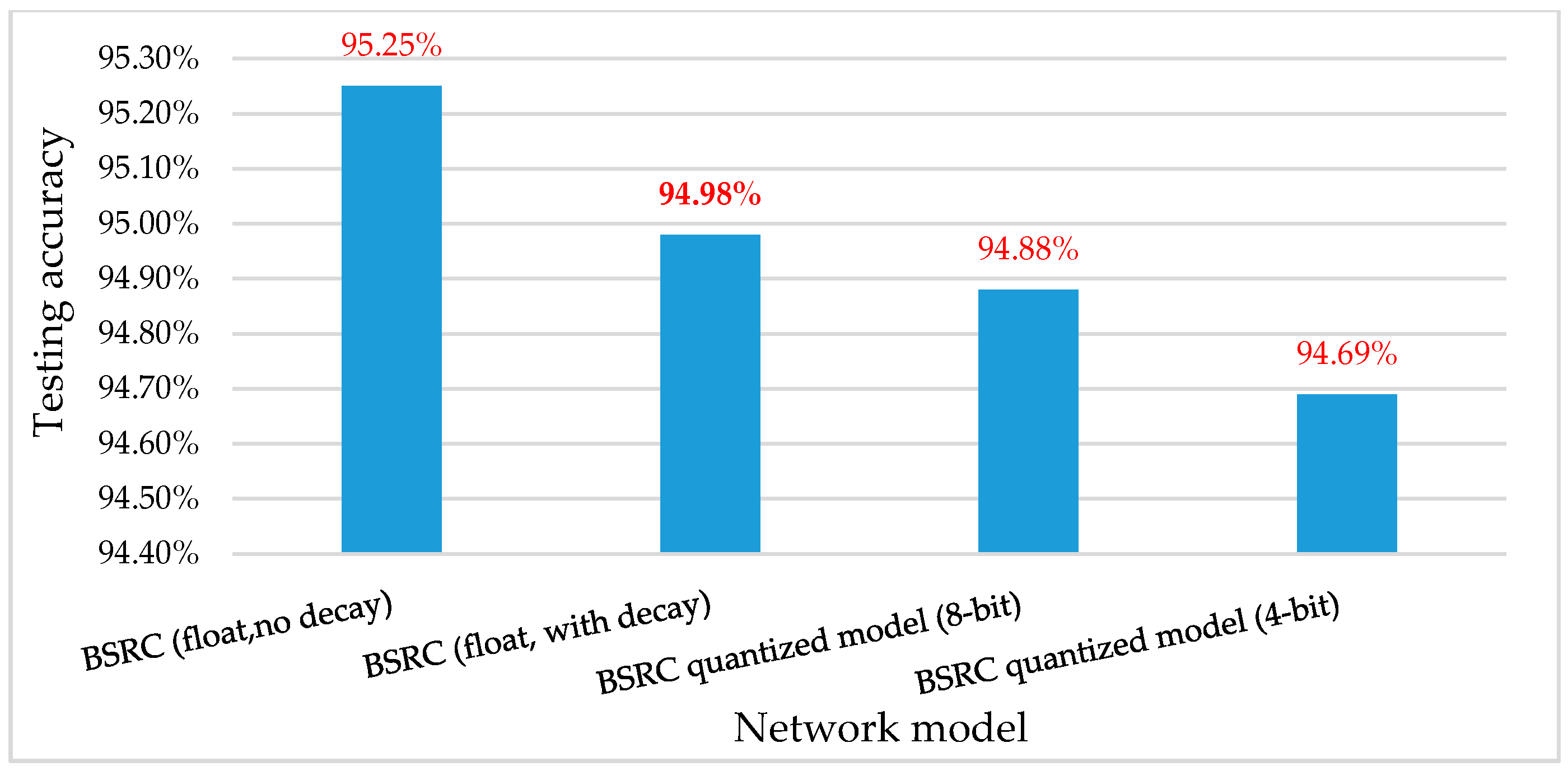
• The target accuracy for MNIST is 94.60% or higher.

The structure optimization process explores SNN structures of various image size, various number of layers, and each layer size in the number of nodes. For the image size, we explored three different image sizes: 28 × 28, 14 × 14, and 9 × 9 by scaling the MNIST dataset. Figure 4 shows three SNNs models using the different image sizes and the accuracy obtained for the each SNNs model using the proposed BSRC based training method described above. The training was conducted with floating-point weight values before applying our weight quantization algorithm. The hardware cost of the three SNNs models in terms of the number of synapses decreases from (635,200) to (164,800), and then to (72,800), which corresponds to 75% and 88.54% reduction, respectively. From this structure optimization, we can observe that resizing the input images to 9 × 9 pixels presents significant size reduction at a negligible accuracy loss (only 0.84%). The next structure optimization is reducing the number of neurons in the hidden layers to determine the minimum network size that meets the target accuracy. For example, Figure 5 compares the maximum testing accuracy of SNNs with various number of neurons in the hidden layer using 9 × 9 MNIST dataset. For SNNs with the hidden layer size ranging from 800 to 50 neurons, the accuracy changes from 98.0% to 95.87%. This indicates that a substantial reduction of 72,800 to 4550 synapses (93.75% reduction) can be obtained at an accuracy loss of only 2.13%.

For a further reduction in the overall hardware cost, we explore SNN structures by splitting the hidden layer into two layers. Figure 1b shows such an SNN constructed by hidden layer splitting. Figure 6 shows various SNN structures by splitting the hidden layer into two hidden layers with various ratios of number of neurons. We can observe that accuracy decreases as we further reduce the total number of synapses. For the running example, we chose the SNN of (81-30-20-10) as the target SNN structure to meet the final accuracy goal of 94.60%.

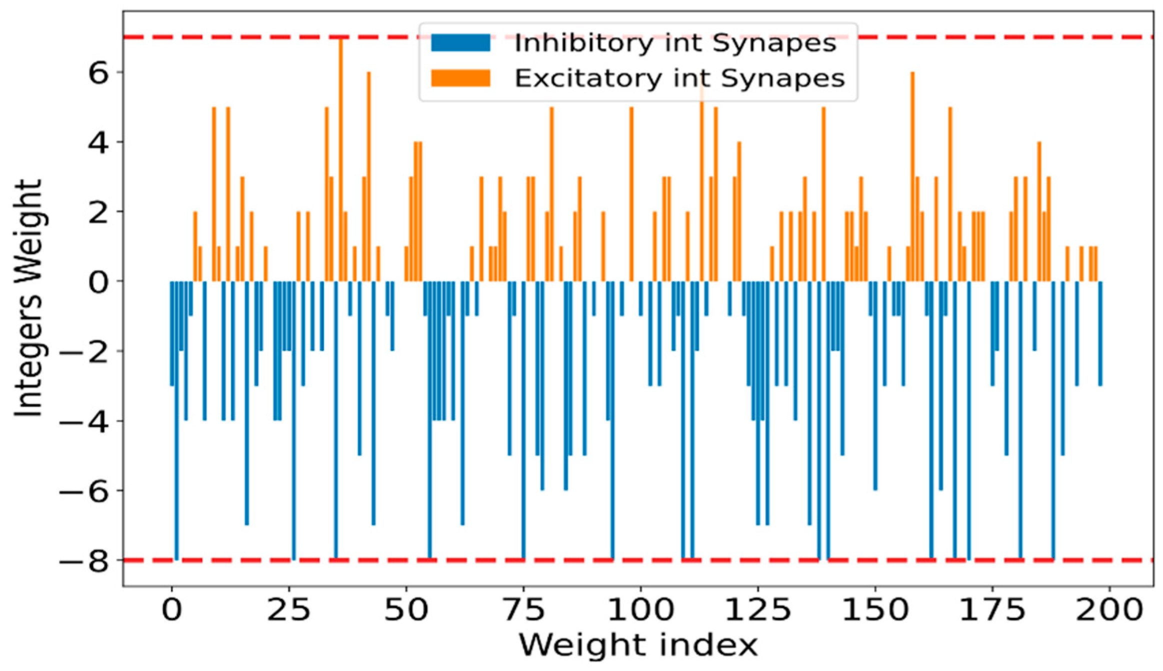
3.3. SNN Weight Quantization

After the iterative process of structure optimization and training, our optimization method applies a weight quantization algorithm to the trained SNN of selected structure to further reduce the circuit size and power consumption. To explain our weight quantization algorithm, we chose an SNN of (81-30-20-10) from the training and structure optimization results of Figure 6 (highlighted in blue color).

In the SNN model considered, every synapse consists of two types of weights:

• Positive weights for Excitatory Synapses
• Negative weights for Inhibitory Synapses

Upon receiving each spike signal, an excitatory synapse increases the spiking rate, while an inhibitory synapse decreases the spiking rate. For each synapse type, the quantization algorithm calculates the mean and the standard deviation of the trained weights that are initially in floating-point. The proposed quantization algorithm determines the optimal range of the weights for each layer based on the mean and standard deviation of floating-point weights. It then clips the weights of each layer by selecting two limits, a positive limit for excitatory synapses and a negative limit for inhibitory synapses. Algorithm 2 summarizes the key steps of our weight quantization algorithm. The selected clipping limits influence the final accuracy. Thus, Algorithm 2 determines the clipping limits for each layer in a way that maximizes the overall SNN’s accuracy.

Algorithm 2 Find optimal Weight Quantization

Inputs: SNN with floating-point weights w, Target Accuracy ATarget, Max allowable number of bits Bmax for quantization Output: The number bits N, Quantized weights wExc _int and wInh_int 1. for $l=0$ $to$L // L is the num. of layers // Group all weights into excitatory and inhibitory weights 2.  for $i=0 to len\left(w\right);$ 3.   if $w$[i] ≥ 0 then wExc = $append\left(w\left[i\right]\right)$; 4.   else wInh = $append\left(w\left[i\right]\right)$;   // Compute statistics of all weights in floating point: 5. MExc= mean(wExc); StdExc= std(wExc); 6. MInh= mean(wInh); StdInh = std(wInh); 7. Repeat for all (nExc, nInh) in range (nmin, nmax) with step (nstep) // Gradually increase the quantized weight resolution: 8.  LExc = nExc $\times$ StdExc + MeanExc; 9.  LInh = nInh $\times$ StdInh + MeanInh; 10.  for $i=0 to len\left(w\right);$ 11.   if   $w$[i] > LExc then $w$[i] = LExc; // Clip the max value 12.   else if $w$[i] < LInh then $w$[i] = LInh; // Clip the min value 13.  for N $=0$ $to$Bmax// Find the best quantization bits N // Calculate the quantization step 14.   ΔExcq = LExc/(2N−1−1); 15.   ΔInhq = LInh/(2N−1);   // Quantize all clipped weights to N-bits 16.   for $i=0 to len\left(w\right);$ 17.     if $w$[i] ≥ 0 then wQ_int[i] = int ($w$[i] /ΔExcq); 18.     else      wQ_int[i] = int ($w$[i] /ΔInhq); 19.   $V_{th\left(int\right)\left(l\right)}$ = Comp_Thresh (wQ_int) 20.   Acc = Calculate Accuracy of SNN (wQ_int) 21. Select best (nExc, nInh) with min N that meets ATarget

Lines 2–4 of Algorithm 2 start by splitting the trained floating-point weights to excitatory and inhibitory weights. For each of weights, Lines 5 and 6 compute the mean and standard deviation. Meanwhile, lines 7–12 iteratively determine the minimum clipping limits of the weight groups, so we can maximize the resolution of the quantized weights by clipping large outlier weights. Lines 14 and 15 calculate the excitatory and inhibitory quantization steps (ΔExcq, ΔInhq) based on the chosen number of bits N for weight quantization. Then, lines 16–21 determine the minimal number of bits for the quantized weights in each layer that can satisfy the target accuracy in the constraints.

To apply Algorithm 2 to the running example SNN of (81-30-20-10), we chose n_min = 0.8, n_max = 1.6, n_step = 0.1, and B_max = 8. As optimal parameters, Algorithm 2 selected n = 4 bits for all layers, clipping limits of (1.04, −1.03) for hidden layer 1, (0.95, −1.19) for hidden layer 2, and (1.24, −2.20) for the output layer. Figure 7 shows the output layer floating-point weights, in this figure the two horizontal red lines indicate the range of floating-point weights before weights clipping. The purple and gray lines (at 1.24 and −2.20) in Figure 7 and Figure 8 are two examples for the chipping levels of excitatory and inhibitory synapses, respectively. Figure 9 shows the SNN output layer 4-bit integers optimized quantized weights according to Algorithm 2.

3.4. Integer Threshold Compensation

The final step of the proposed SNN optimization method is an integer threshold compensation algorithm. After applying the weight quantization algorithm, the floating-point threshold should be compensated to maintain the target accuracy [12,19]. The following equations describe why threshold compensation is required and derive a simplified formula to directly calculate the integer threshold compensation. Equation (7) represents total number of spikes fired by each neuron ($i$) in any layer:

$$N_{Spikes\left(post\right)i}=int\left(\frac{{{\displaystyle \sum }}_{t=0}^{T-1}{{\displaystyle \sum }}_{j=0}^{N_{l-1}^{neurons}-1}\left(w_{ij} · S_j\right)}{V_{th}}\right)$$

(7)

$$F_{r\left(post\right)i}=\frac{N_{Spikes\left(post\right)i}}{T}$$

(8)

In Equations (7) and (8), $N_{Spikes\left(post\right)i}$ is the number of generated spikes in one neuron ($i$), while $F_{r\left(post\right)i}$ indicates the firing rate using floating-point weights for post-neuron ($i$), and $V_{th}$ is the original threshold voltages.

$$N_{Spikes\left(post\right)i}=int\left(\frac{{{\displaystyle \sum }}_{i=0}^{N_l^{neurons}-1}{{\displaystyle \sum }}_{j=0}^{N_{l-1}^{neurons}-1}{w}_{ij}· {{\displaystyle \sum }}_{t=0}^{T-1}\left(S_j\right)}{V_{th}\times T}\right)$$

(9)

$$F_{r\left(post\right)}\simeq \frac{{{\displaystyle \sum }}_{i=0}^{N_l^{neurons}-1}{{\displaystyle \sum }}_{j=0}^{N_{l-1}^{neurons}-1}{w}_{ij}· int\left(\frac{{{\displaystyle \sum }}_{t=0}^{T-1}\left(S_j\right)}{T}\right)}{V_{th}}$$

(10)

$$F_{r\left(post\right)}\simeq \frac{{{\displaystyle \sum }}_{i=0}^{N_l^{neurons}-1}{{\displaystyle \sum }}_{j=0}^{N_{l-1}^{neurons}-1}{w}_{ij}·f_{j-r\left(pre\right)}}{V_{th}}$$

(11)

$$F_{r\left(post\right)}\simeq \frac{ W·F_{r\left(pre\right)}}{V_{th}}$$

(12)

In Equations (9)–(12), by using matrix notations for the weights and input spike streams of all synapses for each neuron, where $F_{r\left(post\right)}$ and $F_{r\left(pre\right)}$ denotes all post-neurons and previous-neurons firing rates matrixes respectively, $N_l^{neurons}$ is the number of neurons in the post layer, $N_{l-1}^{neurons}$ is the number of neurons in the previous layer, while $W$ denotes a floating-point weight matrix. In Equation (11), $f_{j-r\left(pre\right)}$ indicates the firing rate of the spike stream T for each synapse j.

Equation (13) represents an estimation of the firing rate after weight quantization process with N-bits using the integer threshold based on Equation (12).

$$F_{r\left(post\right)-int}\simeq \frac{W_{int } ·F_{r\left(pre\right)-int}}{V_{th-int}}$$

(13)

here, $W_{int}$ represents a matrix of N-bit quantized weights, while $V_{th-int}$ denotes the target threshold to be compensated in integer value for the current layer, while $F_{r\left(pre\right)-int}$ and $F_{r\left(post\right)-int}$ indicate the pre-synaptic firing rate and post-neuron firing rate, respectively.

The goal of our threshold compensation algorithm is to determine an integer threshold $V_{th-int}$ for quantized weights such that the firing rates of Equations (12) and (13) best match; this goal is expressed by Equation (14).

$$\frac{W_{int} ·F_{r\left(pre\right)-int}}{V_{th-int}}\approx \frac{W·F_{r\left(pre\right)}}{V_{th}}$$

(14)

To determine a fast solution that satisfies Equation (14), we assume that $F_{r\left(pre\right)-int}$ equals $F_{r\left(pre\right)}$ (pre-synaptic firing rates before and after weight quantization), which derives a solution expressed by Equation (15):

$$V_{th-int}\approx V_{th} \times \frac{W_{int}}{ W}$$

(15)

To further speed up the computation, we simplify Equation (15) by Equation (16). Equation (16) enables a simple and fast method to find one common threshold (per layer) for all neurons for each network layer:

$$V_{th-int}\approx \lceil V_{th}\times \left|mean\left(\frac{sum\left(W_{int}\right)}{sum\left(W\right)}\right)\right|\rceil$$

(16)

Algorithm 3 summarizes the threshold compensation process for an SNN model of L layers. Line 2 reads the floating-point and integer weights for the entire layer. In line 4, the algorithm divides the accumulated (floating-point and integer) weights for each neuron (i) in the current layer l. Line 5 incrementally calculates the absolute mean of appended results from line 4; the algorithm uses Equation (16) to calculate the compensated integer threshold $V_{th-int\left(l\right)}$ for each layer l.

Algorithm 3 Integer Threshold Compensation

Inputs: Trained SNN quantized with N-bits (integer weights), number of layers $L$, number of neurons $N_l^{neurons}$ in each layer l, $V_{th}$ in floating point, floating-point weights. Outputs: Integer thresholds $V_{th-int\left(l\right)}$ for each layer 1. for l $=0 to \left(L-1\right)$// Calculate $V_{th\left(int\right)\left(l\right)}$ for each layer 2.   Read floating-point and integer weights; // $W_{int}$,$W$ 3.   for $i=0 to N_l^{neurons}$//Divide the accumulated weights for each neuron 4.     $W_{div}\left[i\right]=append\left(\frac{sum\left(W_{int}\left[:,i\right]\right)}{sum\left(W\left[:,i\right]\right)}\right)$ 5.   $V_{th-int\left(l\right)}=\lceil V_{th}\times \left|mean\left(W_{div}\left[0:N_l^{n-1}\right]\right)\right|\rceil$ // Use Equation (16) 6. Report $V_{th\left(int\right)\left(l\right)}$ for each layer

4. Performance Evaluation

To evaluate the proposed optimization method for SNN, we compared SNNs of various structures for MNIST targeting minimal hardware cost under a target accuracy constraint. We first analyze the effectiveness of the proposed BSRC SNN model and training method in floating point weights, and then evaluate the proposed weight quantization and threshold compensation method.

Figure 10 summarizes the accuracy of two SNN structures trained using the proposed BSRC method compared to the previous works in [1,22]. When we apply the proposed BSRC method to an SNN structure of (784-800-10) with floating-point weights using the full-scale MNIST dataset, the model achieves an accuracy of 98.84% after only 84 epochs. In contrast, the previous works, HM2-BP [22] and STBP [11] require 100 and 200 epochs, respectively, to obtain the same level of accuracy for the same SNN structure. For a reduced SNN structure of (784-400-10), BSRC outperforms STBP [11] by 0.3% in accuracy with a training of 43 epochs. This evidence proves the effectiveness of the proposed spike representation and SNN training method. Next, we compare the SNN structural optimization targeting a hardware cost reduction up to the order of 3. We first shrink the input layer size to 9 × 9 MNIST images and follow by minimizing the number of neurons in each layer. Figure 11 compares the accuracy and network size (number of synapses and neurons) for various SNN structures by varying the size of two hidden layers. We chose (81-30-20-10) as the final SNN structure which reduces the number of neurons to 3230 compared with 4550 neurons for the SNN of (81-50-10) at a cost of only 0.7% loss in accuracy.

Figure 12 compares the accuracy of the reduced SNNs (81-30-20-10) obtained via our quantization algorithm. First, note that before the quantization step, the SNN with no decay factor (no leaky component) leads to an accuracy that is 0.27% higher than the SNN with decay factor. This result demonstrates that our simplified neuron model with no decay factor (see Equation (4)) has no accuracy loss. Figure 12 also compares the accuracy of optimized SNNs before and after weight quantization, which proves the effectiveness of our weight quantization method. For example, while the SNN (81-30-20-10) with floating point weight gives an accuracy of 95.25%, the SNNs quantized to 8 bits and 4 bits, respectively, obtain an accuracy of 94.88% and 94.69%. This indicates that a substantial size reduction can be obtained at a negligible accuracy loss.

Figure 13 compares three performance metrics (accuracy, number of synapses, and circuit area) for four different SNNs. The first two groups of bar graphs show the performance metrics of the previous SNNs of 784-800-10 (HM2-BP [22]) and 784-400-10 ( STBP [11]), respectively. These SNNs require a large number of synapses, which lead to excessive hardware cost. Here, the SNN circuit size is represented by the silicon size in mm². In contrast, the third and fourth groups of the bar graphs represent our optimized network structure of (81-30-20-10) for 9 × 9 MNIST images. Compared with the previous SNNs, they drastically reduce the hardware size by 183.19 times (for SNN with floating point weights) and 764.73 times (for SNN with 4-bit quantized weights) at a small accuracy loss of 4.24%, which still satisfies our target accuracy constraint of 94.60%. Compared with HM2-BP SNN of (784-800-10), our SNN of (81-30-20-10) optimized by the proposed BSRC method achieves a significant reduction in the number of synapses from 635,200 to 3230 synapses at a small accuracy loss from 98.93% to 95.25%.

We use Equation (17) to estimate the relative area of the circuit implementation for the SNN model:

$$Circuit Area=\left(N_{syn} \times Siz{e}_{syn}+N_{neuron} \times Siz{e}_{neuron}\right)+H_{w,R}$$

(17)

here, $N_{syn}$ indicates the total number of synapses, while $Siz{e}_{syn}$ represents the total size of synapse circuits including the memories for quantized weights. $N_{neuron}$ denotes the total number of neurons, while $Siz{e}_{neuron}$ indicates the size of a neuron circuit. $H_{w,R}$ is the wiring and routing overhead.

As we can see in Figure 13, the proposed optimization method reduces the hardware area from 3089.49 ${\mathrm{mm}}^2$ for HM2-BP SNN (784-800-10) with 32-bit floating-point weights to 16.86 ${\mathrm{mm}}^2$ for SNN (81-30-20-10) with 32-bit floating-point weights. The 4-bit quantization method provides an additional size reduction of 4 times from 16.86 ${\mathrm{mm}}^2$ to 4.04 ${\mathrm{mm}}^2$ with a negligible accuracy loss of only 0.56%. These implementation and evaluation results demonstrate that the proposed optimization method using BSRC SNN model is a highly effective approach to minimizing the hardware size and tradeoff between accuracy and hardware size.

We implemented the final optimized SNN model BSRC (81-30-20-10) using analog circuits for synapse and neuron cells and digital standard cells for weight and image memories. Figure 14a illustrates the overall block diagram of the SNN chip based on BSRC (81-30-20-10), while Figure 14b shows the full chip layout design of the silicon. The SNN chip is currently under fabrication using CMOS 65 nm process. We plan to report the test results of the silicon in a future paper.

5. Conclusions

Although the artificial neural networks can achieve high testing accuracy for the MNIST dataset, most of these models tend to incur excessive hardware code, and thus are not suitable for edge AI and mobile systems. In this work, we have developed an SNN model and optimization method by introducing a new spike representation scheme called Binary Streamed Rate Coding (BSRC). BSRC improves the model generality, eliminates the need for random noise, and consequently offers efficient training and high accuracy. Our optimization method consists of SNN structure optimization, BSRC spike generation, weight quantization, and threshold compensation algorithms. We applied the proposed optimization method to an SNN for MNIST dataset and obtained 764.73 times reduction in circuit size with accuracy loss of 4.24% compared with the previous SNN reported in [22]. This result envisages that the proposed method can offer a breakthrough to design an extremely compact and low power SNN hardware with a reasonable accuracy aimed at edge AI applications. For future work, we plan to extend the proposed method and apply to a larger SNNs with different datasets such as CIFAR-10 which contain color images and CIFAR-100 for more classes. We also plan to extend it for hybrid neural networks comprising convolutional layers as well as spiking synapse layers.

References

1. Pfeiffer, M.; Pfeil, T. Deep Learning With Spiking Neurons: Opportunities and Challenges. Front. Neurosci. 2018, 12, 774. [Google Scholar] [CrossRef] [PubMed] [Green Version]
2. Pedroni, B.U.; Sheik, S.; Mostafa, H.; Paul, S.; Augustine, C.; Cauwenberghs, G. Small-footprint Spiking Neural Networks for Power-efficient Keyword Spotting. In Proceedings of the 2018 IEEE Biomedical Circuits and Systems Conference (BioCAS), Cleveland, OH, USA, 17–19 October 2018; pp. 1–4. [Google Scholar]
3. Furber, S.B.; Lester, D.R.; Plana, L.A.; Garside, J.D.; Painkras, E.; Temple, S.; Brown, A.D. Overview of the SpiNNaker System Architecture. IEEE Trans. Comput. 2012, 62, 2454–2467. [Google Scholar] [CrossRef] [Green Version]
4. Yan, Y.; Kappel, D.; Neumarker, F.; Partzsch, J.; Vogginger, B.; Hoppner, S.; Furber, S.B.; Maass, W.; Legenstein, R.; Mayr, C.; et al. Efficient Reward-Based Structural Plasticity on a SpiNNaker 2 Prototype. IEEE Trans. Biomed. Circuits Syst. 2019, 13, 579–591. [Google Scholar] [CrossRef] [PubMed] [Green Version]
5. Davies, M.; Srinivasa, N.; Lin, T.-H.; Chinya, G.; Cao, Y.; Choday, S.H.; Dimou, G.; Joshi, P.; Imam, N.; Jain, S.; et al. Loihi: A Neuromorphic Manycore Processor with On-Chip Learning. IEEE Micro 2018, 38, 82–99. [Google Scholar] [CrossRef]
6. Benjamin, B.V.; Gao, P.; McQuinn, E.; Choudhary, S.; Chandrasekaran, A.R.; Bussat, J.-M.; Alvarez-Icaza, R.; Arthur, J.V.; Merolla, P.A.; Boahen, K. Neurogrid: A Mixed-Analog-Digital Multichip System for Large-Scale Neural Simulations. Proc. IEEE 2014, 102, 699–716. [Google Scholar] [CrossRef]
7. Merolla, P.A.; Arthur, J.V.; Alvarez-Icaza, R.; Cassidy, A.S.; Sawada, J.; Akopyan, F.; Jackson, B.L.; Imam, N.; Guo, C.; Nakamura, Y.; et al. A million spiking-neuron integrated circuit with a scalable communication network and interface. Science 2014, 345, 668–673. [Google Scholar] [CrossRef]
8. Xu, Y.; Tang, H.; Xing, J.; Li, H. Spike trains encoding and threshold rescaling method for deep spiking neural networks. In Proceedings of the 2017 IEEE Symposium Series on Computational Intelligence (SSCI), Honolulu, HI, USA, 27 November–1 December 2017; pp. 1–6. [Google Scholar]
9. Brette, R. Philosophy of the Spike: Rate-Based vs. Spike-Based Theories of the Brain. Front. Syst. Neurosci. 2015, 9, 151. [Google Scholar] [CrossRef]
10. Kiselev, M. Rate coding vs. temporal coding-is optimum between? In Proceedings of the 2016 International Joint Conference on Neural Networks (IJCNN), Vancouver, BC, Canada, 24–29 July 2016; pp. 1355–1359. [Google Scholar]
11. Wu, Y.; Deng, L.; Li, G.; Zhu, J.; Shi, L. Spatio-Temporal Backpropagation for Training High-Performance Spiking Neural Networks. Front. Neurosci. 2018, 12, 331. [Google Scholar] [CrossRef]
12. Wu, S.; Li, G.; Chen, F.; Shi, L. Training and inference with integers in deep neural networks. arXiv 2018, arXiv:1802.04680. (preprint). [Google Scholar]
13. Courbariaux, M.; Itay, H.; Daniel, S.; Ran, E.-Y.; Yoshua, B. Binarized neural networks: Training deep neural networks with weights and activations constrained to +1 or −1. arXiv 2016, arXiv:1602.02830. (preprint). [Google Scholar]
14. Han, J.; Li, Z.; Zheng, W.; Zhang, Y. Hardware implementation of spiking neural networks on FPGA. Tsinghua Sci. Technol. 2020, 25, 479–486. [Google Scholar] [CrossRef]
15. Cheng, J.; Wu, J.; Leng, C.; Wang, Y.; Hu, Q. Quantized CNN: A Unified Approach to Accelerate and Compress Convolutional Networks. IEEE Trans. Neural Networks Learn. Syst. 2017, 29, 4730–4743. [Google Scholar] [CrossRef]
16. Wu, J.; Leng, C.; Wang, Y.; Hu, Q.; Cheng, J. Quantized convolutional neural networks for mobile devices. In Proceedings of the IEEE Conference on Computer Vision and Pattern Recognition, Las Vegas, NV, USA, 27–30 June 2016; pp. 4820–4828. [Google Scholar]
17. Choukroun, Y.; Kravchik, E.; Yang, F.; Kisilev, P. Low-bit quantization of neural networks for efficient inference. In Proceedings of the 2019 IEEE/CVF International Conference on Computer Vision Workshop (ICCVW), Seoul, Korea, 27–28 October 2019; pp. 3009–3018. [Google Scholar]
18. Wang, Y.; Shahbazi, K.; Zhang, H.; Oh, K.I.; Lee, J.-J.; Ko, S.-B. Efficient spiking neural network training and inference with reduced precision memory and computing. IET Comput. Digit. Tech. 2019, 13, 397–404. [Google Scholar] [CrossRef]
19. Wang, Y.; Xu, Y.; Yan, R.; Tang, H. Deep Spiking Neural Networks with Binary Weights for Object Recognition. IEEE Trans. Cogn. Dev. Syst. 2020, 1. [Google Scholar] [CrossRef]
20. Courbariaux, M.; Yoshua, B.; Jean-Pierre, D. Binaryconnect: Training deep neural networks with binary weights during propagations. In Advances in Neural Information Processing Systems; Neural Information Processing Systems Foundation, Inc.: La Jolla, CA, USA, 2015; pp. 3123–3131. [Google Scholar]
21. Cao, Y.; Chen, Y.; Khosla, D. Spiking Deep Convolutional Neural Networks for Energy-Efficient Object Recognition. Int. J. Comput. Vis. 2014, 113, 54–66. [Google Scholar] [CrossRef]
22. Jin, Y.; Li, P.; Zhang, W. Hybrid macro/micro level backpropagation for training deep spiking neural networks. In Advances in Neural Information Processing Systems; Neural Information Processing Systems Foundation, Inc.: La Jolla, CA, USA, 2018; pp. 7005–7015. [Google Scholar]
23. Markram, H. Regulation of Synaptic Efficacy by Coincidence of Postsynaptic APs and EPSPs. Science 1997, 275, 213–215. [Google Scholar] [CrossRef] [Green Version]
24. Kheradpisheh, S.R.; Ganjtabesh, M.; Masquelier, T. Bio-inspired unsupervised learning of visual features leads to robust invariant object recognition. Neurocomputing 2016, 205, 382–392. [Google Scholar] [CrossRef] [Green Version]
25. Kistler, W.M.; Van Hemmen, J.L. Modeling Synaptic Plasticity in Conjunction with the Timing of Pre- and Postsynaptic Action Potentials. Neural Comput. 2000, 12, 385–405. [Google Scholar] [CrossRef]
26. Diehl, P.U.; Neil, D.; Binas, J.; Cook, M.; Liu, S.-C.; Pfeiffer, M. Fast-classifying, high-accuracy spiking deep networks through weight and threshold balancing. In Proceedings of the 2015 International Joint Conference on Neural Networks (IJCNN), Killarney, Ireland, 12–17 July 2015; pp. 1–8. [Google Scholar]
27. Sengupta, A.; Ye, Y.; Wang, R.; Liu, C.; Roy, K. Going Deeper in Spiking Neural Networks: VGG and Residual Architectures. Front. Neurosci. 2019, 13, 95. [Google Scholar] [CrossRef]
28. Rueckauer, B.; Lungu, I.-A.; Hu, Y.; Pfeiffer, M.; Liu, S.-C. Conversion of Continuous-Valued Deep Networks to Efficient Event-Driven Networks for Image Classification. Front. Neurosci. 2017, 11, 682. [Google Scholar] [CrossRef]
29. Mostafa, H.; Pedroni, B.U.; Sheik, S.; Cauwenberghs, G. Fast classification using sparsely active spiking networks. In Proceedings of the 2017 IEEE International Symposium on Circuits and Systems (ISCAS), Baltimore, MD, USA, 28–31 May 2017; pp. 1–4. [Google Scholar]
30. Mostafa, H. Supervised Learning Based on Temporal Coding in Spiking Neural Networks. IEEE Trans. Neural Networks Learn. Syst. 2017, 29, 3227–3235. [Google Scholar] [CrossRef] [PubMed] [Green Version]
31. Burkitt, A.N. A Review of the Integrate-and-fire Neuron Model: I. Homogeneous Synaptic Input. Boil. Cybern. 2006, 95, 1–19. [Google Scholar] [CrossRef] [PubMed]
Figure 1. Spiking neural network (SNN) structure: (a) SNN structure (m hidden layers) for Modified National Institute of Standards and Technology (MNIST) dataset 28 × 28; (b) SNN structure (two hidden layers) for MNIST dataset 9 × 9. In the (a,b), red synapse color represents Excitatory synapses and blue for Inhibitory one, the bold line indicates more positive (Excitatory) or more negative (Inhibitory) values.
Electronics 09 01599 g001
Figure 2. (a) ANN neuron model; (b) SNN neuron model.
Electronics 09 01599 g002
Figure 3. 4–bit pixels, Binary Streamed Rate Coding (BSRC) conversion results.
Electronics 09 01599 g003
Figure 4. Testing accuracy of SNNs with one hidden layer of 800 nodes. BSRC (28 × 28 − 14 × 14 − 9 × 9) 4-bit per Pixel.
Electronics 09 01599 g004
Figure 5. Maximum testing accuracy of SNNs with one hidden layer of (800 to 50) neurons.
Electronics 09 01599 g005
Figure 6. Maximum testing accuracy of SNNs with two hidden layers using various structures.
Electronics 09 01599 g006
Figure 7. SNN output layer 32-bit floating-point weights (Excitatory weights = 46.5% and Inhibitory weights = 53.5%).
Electronics 09 01599 g007
Figure 8. SNN output layer 32-bit floating-point weights after clipping the outlier excitatory and inhibitory weights to increase integer weight resolution.
Electronics 09 01599 g008
Figure 9. SNN output layer 4-bit integers weight ranged from (−8) to (7) as shown in the two red horizontal lines, the integers weights optimized according to Algorithm 2.
Electronics 09 01599 g009
Figure 10. Accuracy of two SNN structures trained by three different modeling and training techniques: HM2-BP, STBP, and BSRC (Proposed).
Electronics 09 01599 g010
Figure 11. Binary Streamed Rate Coding (BSRC) accuracy and number of synapses for two hidden layers SNN.
Electronics 09 01599 g011
Figure 12. Accuracy of SNNs with optimized structure (81-30-20-10) trained with decay factor = 1 (no decay), decay factor = 0.5, and quantized weight (8-bit and 4-bits) resolutions.
Electronics 09 01599 g012
Figure 13. SNN circuit area mm 2 and accuracy using different models.
Electronics 09 01599 g013
Figure 14. (a) The overall block diagram of the SNN chip optimized with BSRC 81-30-20-10 (4-bit quantized); (b) The full chip layout photo of the SNN chip under fabrication.
Electronics 09 01599 g014