Characterizing the Effect of Conservation Voltage Reduction on the Hosting Capacity of Inverter-Based Distributed Energy Resources


1
ATCO, Edmonton, AB T5j 2V6, Canada
2
AESO, Calgary, AB T2P 0L4, Canada
*
Author to whom correspondence should be addressed.
Electronics 2020, 9(9), 1517; https://doi.org/10.3390/electronics9091517
Submission received: 15 August 2020
/
Revised: 3 September 2020
/
Accepted: 10 September 2020
/
Published: 16 September 2020
(This article belongs to the Special Issue Smart Inverters in Power Grids and Renewable Energy Systems)
Abstract
:The increased adoption of inverter-based distributed energy resources in the form of the mass deployment of renewable generation systems has been a focal goal of many jurisdictions worldwide. Actions taken by local governments have included adapted regulations, financial subsidies, and a variety of grants. This has spurred the proliferation of solar generation among residential customers in virtually all provinces of the United States and Canada. Needless to say, these small generators are interfaced with DC–AC inverters, which have evolved tremendously since the formation of working groups targeting the impact of inverter-based generation on the grid. Among the first rules and standards are California’s ISO Rule 21 and the UL1741 SA, which were published in September 2017. IEEE followed suit in 2018 with the revision of IEEE 1547, inspiring virtually all jurisdictions to either adopt these standards or adapt them as their own variants. Among many features, these standards mandate inverters to be fitted with autonomous performance functions, including the constant power factor, voltage-reactive power (Volt-VAR), voltage-active power (Volt-Watt), and grid support functions, as well as provisions for compatibility with control centers. These functions have been demonstrated to increase the nameplate hosting capacity. At the same time, grid modernization strategies have become more prevalent, one of which is the use of conservation voltage reduction. This grid modernization initiative has a great impact on the hosting capacity. Conversely, the increased penetration of distributed energy resources has a negative effect on the conservation voltage reduction, but surprisingly to only a limited extent. The characterization of these impacts is addressed in this paper, with a focus on a case with very high DER penetration and with very long daily sunlight hours.
1. Introduction
Distributed energy resources (DERs) have experienced rejuvenated interest over the past two decades, since the process of deregulation began for electric utilities. Recently, this interest has gained increased momentum, propelled by government initiatives, such as grants and changing regulations. DERs, especially those that are renewable-based, have the potential to reduce greenhouse gases if employed in areas reliant on burning fuel. If coupled with energy storage, they also have the potential to alleviate congestion and even allow electric utilities to defer infrastructure investment. From the prosumer standpoint, DERs can also allow reduced grid reliance and potential capitalization on government grants [1,2]. As a result, the number of residential-scale photovoltaic (PV) generators has grown tremendously and continues to boast an upward trend. Some states in the US and countries in Europe have experienced so much uptake that technical problems have appeared, ranging from reduced inertia to inability to ideally manage voltage in distribution systems.
To improve the lack of DER controllability and reduce the negative impacts of DERs, many task forces have been developed to impose stricter requirements on inverters. One of the precursors was chaired by the California Independent System Operator (ISO), which developed Rule 21 [3]. This document paved the way for the revision of interconnection standards around the world, such as the Underwriter Laboratories 1741 Supplement Addendum [4], the Institute of Electrical and Electronics Engineers Standard 1547-2018 [5], and the Canada Standards Association Standard C22.3 number 9:20 [6]. Similarly, the IEEE revised the test procedure requirements in [7] to ensure unification in functions that need to be tested. A major benefit of all these efforts is that the PV hosting capacity can be greatly expanded, with a somewhat controllable negative impact on the high penetration of DERs at the expense of mandatory reactive power management or active power curtailment.
Meanwhile, there have been great strides made in smart grid initiatives, many of which are tailored to incorporate the high penetration of DERs. For example, most commercially advanced distribution management systems (ADMS) also offer a DER management system (DERMS) module to include visibility and the control of DERs in distribution grid management. While most utilities around the world are not yet users of ADMS and DERMS, these systems are part of most utilities’ grid modernization plans. One established technology that has made its way into most ADMS offerings is conservation voltage reduction (CVR). This technique has been identified as a way to reduce load consumption since the 1970s [8] and has been employed by US utilities since the 1980s [9]. CVR, while being an obvious contender to reduce energy consumption, is not an intuitive application, because in most distribution systems the wire owner will try to boost the voltage to account for voltage drop due to line losses, representing a fine balance that can only be achieved if carefully planned and executed. With the increasing penetration of DERs, however, researchers have noted the potential interaction of CVR and DERs, as presented in [10,11,12]. The authors of [10] analyzed two weeks of randomly generated data for the IEEE 13-bus system and concluded that the high penetration of DERs can negate the benefits of CVR. Similarly, the authors in [11] used a test system to arrive at a similar conclusion but extended the analysis to different load compositions. The authors of [12] characterized how DERs can improve the power quality of systems where CVR is implemented, resulting in potentially more aggressive CVR settings without compromising power quality. Furthermore, studies such as [13,14] have proposed energy management systems in microgrids that can not only manage the large penetration of renewable energy sources, but can also optimize the energy consumed. These ideas are paving the way for extremely intelligent energy management systems but are not building upon products that are commercially available today.
Past research, while very insightful, has not directly addressed the impacts of a commercial CVR on the DER hosting capacity under the scenarios that electric utilities face today, where DER real-time data are not available to the system operator yet (with exceptions). This paper presents these impacts as faced by a Canadian electric utility. To achieve this, one of the utility’s urban feeders is used as a case study. Different levels of CVR settings are used and the impact on the hosting capacity is assessed (i.e., how much DERs can output) with the implementation of smart inverter functions (voltage-reactive power (Volt-VAR) and voltage-active power (Volt-Watt) are used). In addition, as with [10,11], this paper also assesses the impact of the mass adoption of DERs on the effectiveness of CVR. The main focus of this paper is the strategy employed, which results in very striking conclusions. Mainly, the implementation of a CVR scheme can be very beneficial. It has the potential to substantially increase the hosting capacity, but interestingly high DER penetration does not negate the effectiveness of the CVR scheme. In other words, CVR enables higher DER nameplate installation with very little impact on energy savings, making CVR a suitable grid modernization strategy for DER-rich systems. This is especially true in systems such as the one used in this paper, that of a northern electric utility that experiences very long sunny days during the summer. The paper is structured as follows. Section 2 provides a brief background on the problem of voltage rise due to DERs and their smart inverter performance functions. Section 3 provides a brief overview of CVR, as well as the load composition. Section 4 presents the system under study and simulation studies. Section 5 concludes the paper.
2. Voltage Rise and Smart Inverter Voltage Control Functions
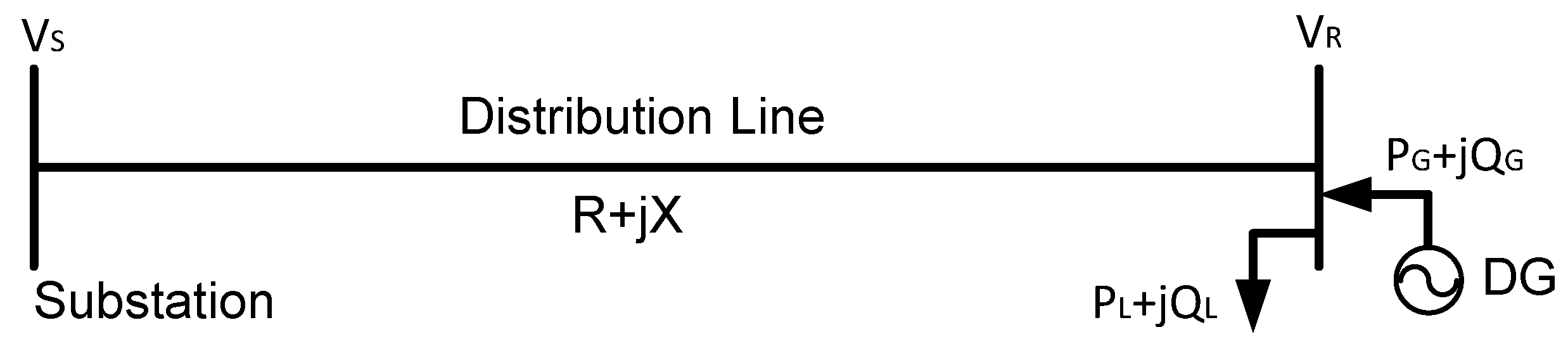
When connected to distribution feeders, DERs typically raise the voltage near their interconnection point. In fact, this has been identified as the biggest challenge when connecting DERs [15]. The system presented in Figure 1 is being used to explain this challenge.
The distribution line illustrated in this example will experience a voltage rise given by
When generation exceeds at the receiving end, (PL − PG) × R results in negative value, and ΔV also becomes negative due to the voltage rise experienced at the DER terminal. The DER can counteract this effect by absorbing reactive power QG, but this action is limited as large injections of QG translate into reduced PG, as inverter-based generators are limited by the ampacity rating of their inverter transistors, which determines the inverter rating.
To further illustrate this effect, if we were to maintain the terminal voltage constant, ΔV would be zero and
Typical distribution conductors have low R/X. An example is the most prevalent conductor used in distribution lines, namely 1/0 ACSR, which has R/X ≈ 1. With such low ratio, to completely negate the effect of each Watt on the terminal voltage, the same number of VARs would need to be absorbed. Such an under-excited mode is not possible with neither inverter-based nor synchronous generation.
However, smart inverter functions, now dictated by [3,4,5,6,7], have the potential to reduce this negative impact of DERs on grid voltage. The most common functions, which are investigated in this paper, are explained as follows.
2.1. Adjustable Power Factor Mode
The requirement of operating under constant power factor is the classical and most common requirement in most jurisdictions in North America, due to the fact the utilities still have the need to control voltage in the systems in which they operate. This mode requires the DER to operate under constant power factor regardless of its instantaneous active power output. Most, if not all, PV inverters are manufactured with the default setting of unity power factor, should the function be enabled. For this reason, when simulated under constant power factor mode, this paper assumes that all PV inverters will be operating under unity power factor.
2.2. Adjustable Volt-VAR Mode
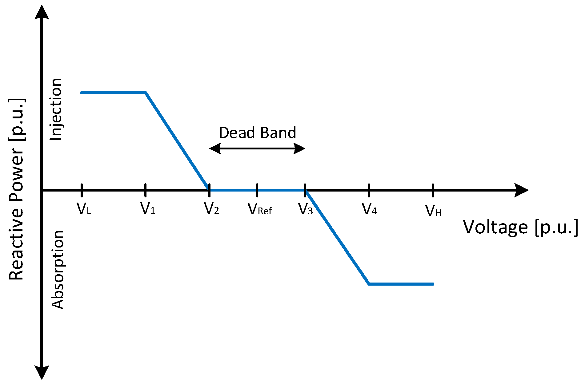
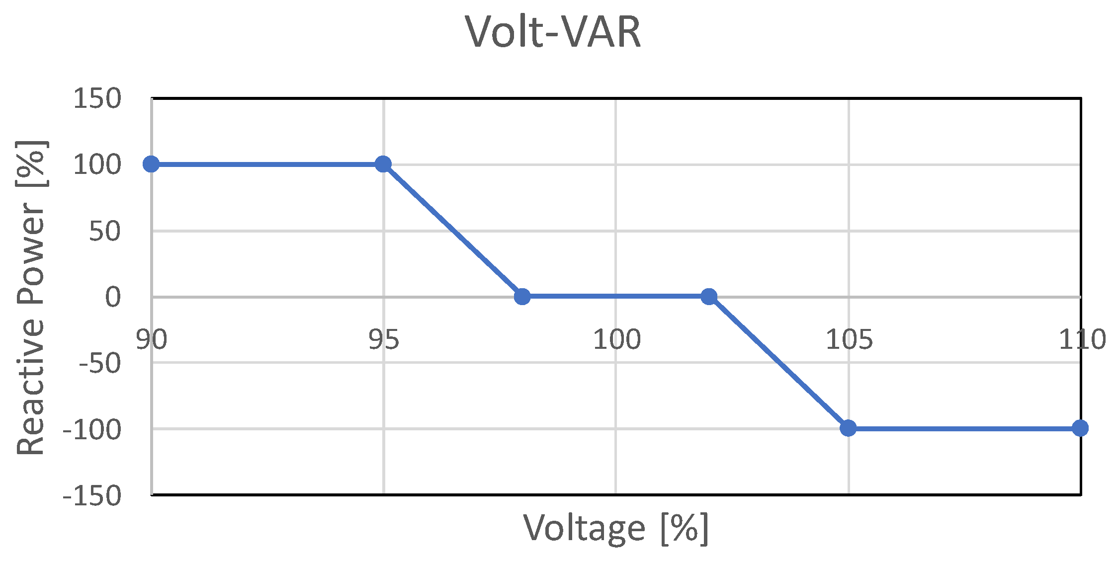
The Volt-VAR mode, especially the Volt-VAR with Watt priority (VV11 convention), has recently been gaining widespread acceptance as utilities start to allow DERs to control voltage. When in this mode, the DER controls its reactive power output as a function of voltage following a Volt-VAR characteristic, such as that shown in Figure 2.
2.3. Adjustable Volt-Watt Mode
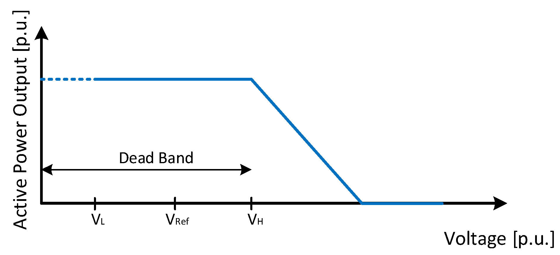
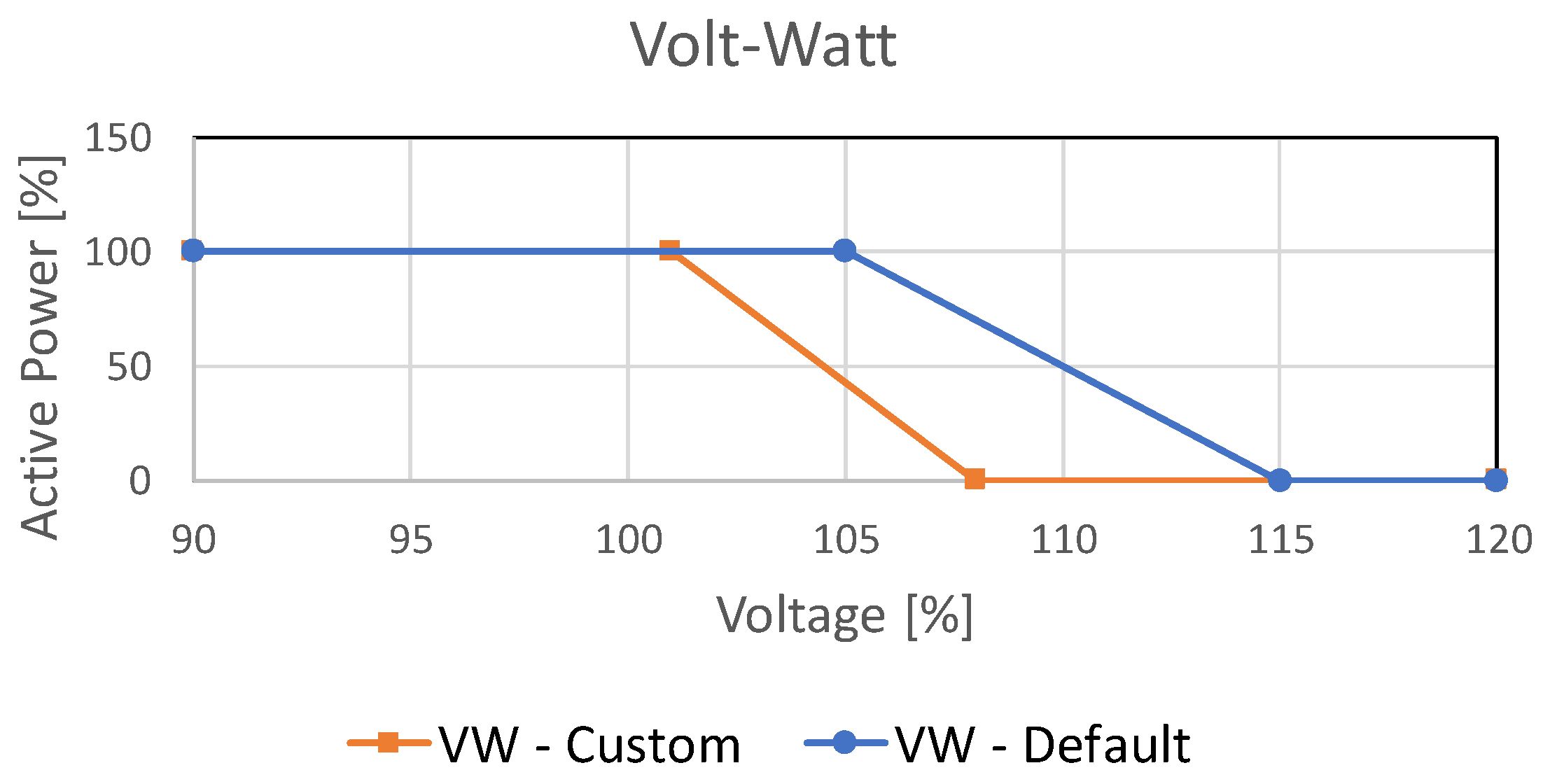
The Volt-Watt mode is an operational model that is very effective in managing very localized voltage. Typically, this mode does not introduce voltage management challenges to the system operator because DERs are planned in a way that their active power output has no impact, except for rapid changes that may cause light flicker. When in this mode, the DER controls its active power output as a function of voltage following a Volt-Watt characteristic, such as that shown in Figure 3. This means that under high voltage scenarios, the DER will curtail its active power output.
3. CVR and Electrical Load Composition
CVR is a very well-known technique to reduce energy consumption and is based on the premise that a reduction in voltage will lead to a corresponding reduction in energy consumption by the end-use loads. However, the application of CVR was initially very controversial and did not initially gain acceptance, due to: (1) potentially causing a reduction in revenue by the local utility; (2) potential power quality problems resulting from imposing voltages of low magnitude voltages on customer load; (3) some types of load that may actually increase their energy consumption under low voltage conditions [16].
3.1. CVR Principle and Definition
The fact of the matter is that the CVR principle is that energy can be saved while not violating voltage limits by operating in the lower half of the ANSI residential voltage band (i.e., 114 V to 120 V rather than 120 V–126 V). The CVR factor was developed as a measure of how effectively a voltage reduction can be in reducing energy consumption, which can be mathematically expressed as
3.2. Electrical Load Composition
Extensive research in the past has shown that the composition of the load can affect its behavior, and consequently it is important to characterize the load when employing CVR. In most load flow software packages, the loads can be modeled as either polynomial or exponential. Other models that include frequency dependence also exist but are not typically present in these software packages. The composite polynomial model can be expressed as
where kn is the polynomial load composition coefficients—namely k1 and k4 are the portions of constant impedance, k2 and k5 are the portions of constant current, k3 and k6 are the portions of constant power, P0 and Q0 are the nominal real and reactive power, and V0 is the nominal voltage. All parameters are represented in per unit (p.u.). Of note, k1 + k2 + k3 = 1 and k4 + k5 + k6 = 1.
The exponential model, on the other hand, reads as
where nP and nQ are the real and reactive exponent factors in p.u. To note, nP or nQ = 0 for constant power loads, 1 for constant current loads, and 2 for constant impedance loads.
4. Characterization of the Impact of CVR on DER Hosting Capacity
This section focuses on the characterization of the impact of CVR on the Hosting Capacity of DERs, and on the impact of the high penetration of DERs on the CVR effectiveness. The analysis was conducted on an urban feeder where the utility has experienced substantial uptake of microgeneration and anticipates that this will continue. Among several smart grid initiatives, the utility is considering the adoption of CVR, and this paper characterizes some of the studies conducted to date. The paper studies the various available smart inverter modes and their interaction with the scheme, analyzes the impact of load composition, and quantifies energy saving as a result of these sensitivity variations.
4.1. The System under Study
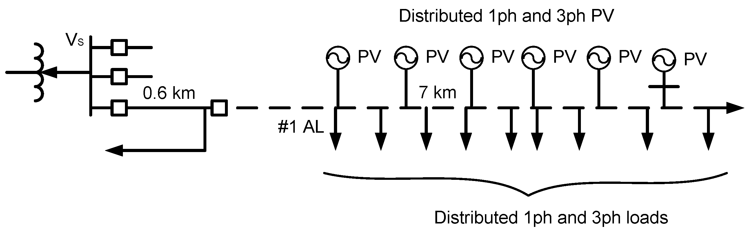
In this study, the three inverter autonomous modes presented in Section 2 were implemented to allow assessing the impact of CVR on PV penetration levels. A real feeder supplying the city of Fort McMurray was used to conduct this study. This system is mainly residential and commercial, is radial in nature and about 8 km in length. It is predominantly underground, composed by jacketed #1 aluminum underground cables, which have R/X ≈ 1.2. It supplies 3858 customers and about 10MW peak load among single- and three-phase customers. The load distribution was obtained from the Customer Information System (CIS) and allocated as per the Geographic Information System (GIS). This modeling is done automatically but the software suite integrates and interconnects all these systems. The historical feeder loading, which is collected at the feeder header by a revenue meter, is updated every 15 min and stored in the Meter Data Management (MDM) and used to scale all loads proportional to their peak consumption. Then, each four 15-min interval was averaged to obtain an hourly profile. This procedure allows for solving a time-series load flow that takes into account instantaneous load demand. This system is illustrated in Figure 4.
It was assumed the PV generators were randomly distributed and that the penetration reached about 50% of the peak load, or about 5 MW. The random DER interconnections were either residential (single-phase) or commercial (three-phase) connected generators. A high-level analysis of potential locations was completed, taking into account the existing Microgeneration regulation in Alberta [17], where customers connecting an amount of renewable generation not exceeding 5 MW in nameplate and not having energy production exceeding annual energy consumption, would qualify for special treatment; hence, they have a higher likelihood to propose such interconnection.
The system was modeled in CYMDIST, part of the CYME suite. The Long-Term Dynamics module was used to incorporate an hourly profile of the feeder and hourly solar irradiation profile in the region. The solar irradiation data were downloaded from the NASA database for the past 15 years and a 15-min average profile was obtained. This profile was inputted in the aforementioned module. Then, each four 15-min interval was averaged to obtain an hourly profile. The CYME Long Term Dynamics Module can solve a load flow solution, incorporating inverter control functions, every hour. For ease of illustration, most results were derived for the month of June, which has the greatest insolation and most noticeable impact. In Canada, it also represents a month of light load consumption, as it is warm (and air conditioners are not common in this city due to its northern location).
4.2. The Impact of CVR on the Base Case
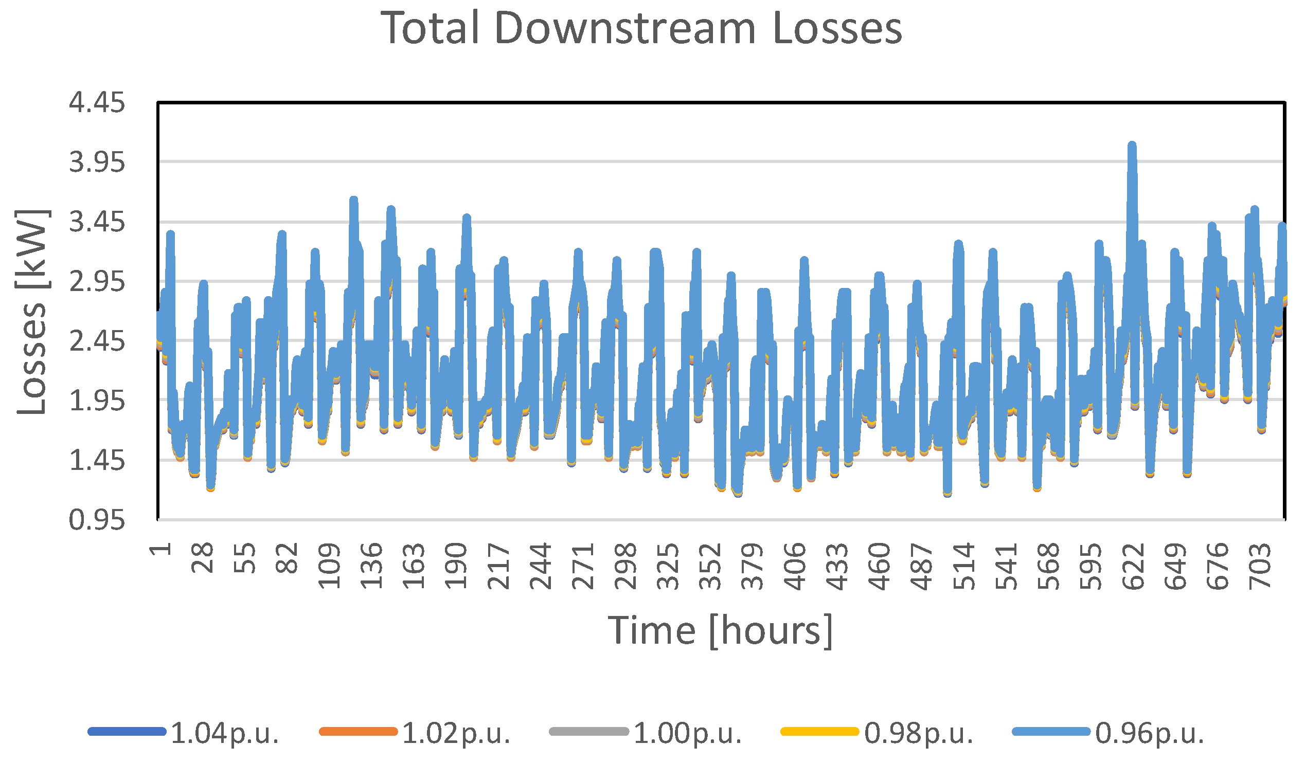
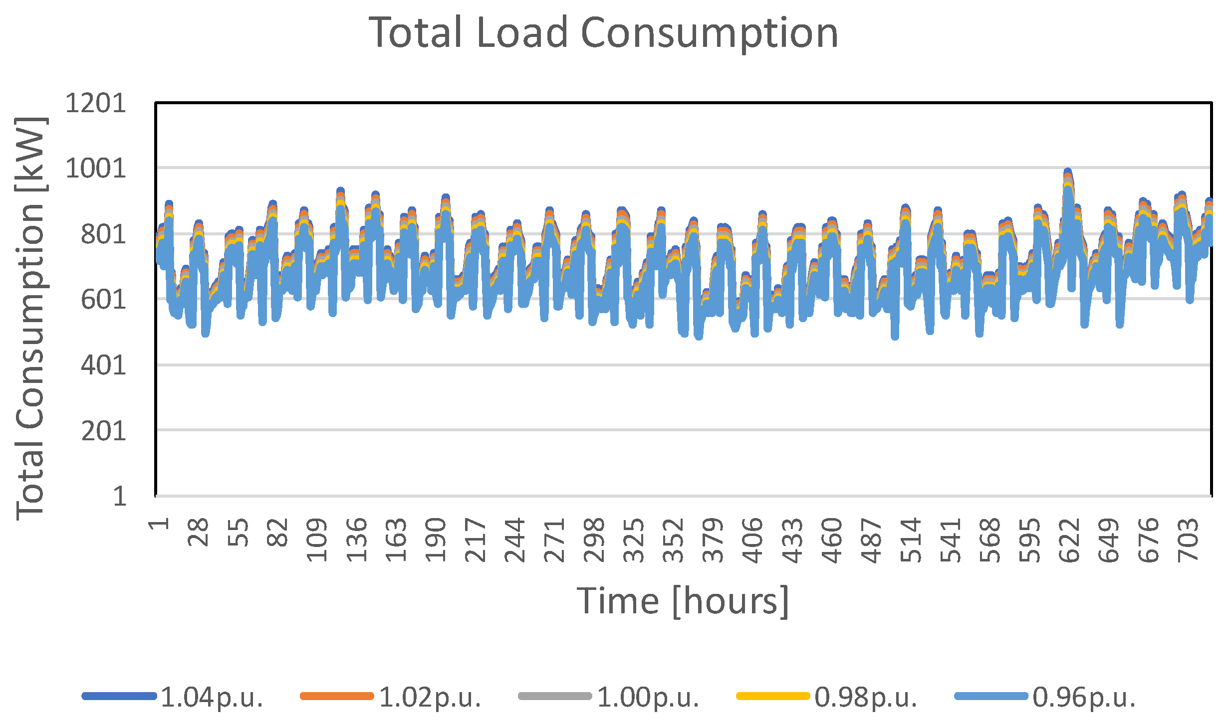
The effect of CVR was simulated for the feeder as it exists today. The standard constant power load model was used. Both the instantaneous total downstream line losses and load consumption were calculated by using the load flow software and recorded, plotted in Figure 5 and Figure 6, respectively. The strategy was to run a time-series hourly load flow for each hour of the month, calculate the hourly line losses and energy consumption, and report in these two figures. While difficult to see clearly in Figure 5, the lower the CVR setpoint (lower the voltage), the higher the line technical losses. However, Figure 6 suggests a noticeable reduction in consumption in the lower the adopted CVR setpoint.
To note, the CVR was employed to allow a 4% voltage reduction from nominal voltage (115 V on a 120 V basis) as employed at the primary side of the load (in this case, on the 25 kV system), being the minimum acceptable voltage. For a typical transformer, which has %IZ = 4%, this could result in a service entrance as low as 110 V, which is the minimum allowed voltage as prescribed in [17]. Hence, as per the simulation results conducted in this work, no CVR setpoints lower than the ones used to obtain those termed “0.96 p.u.” are allowed.
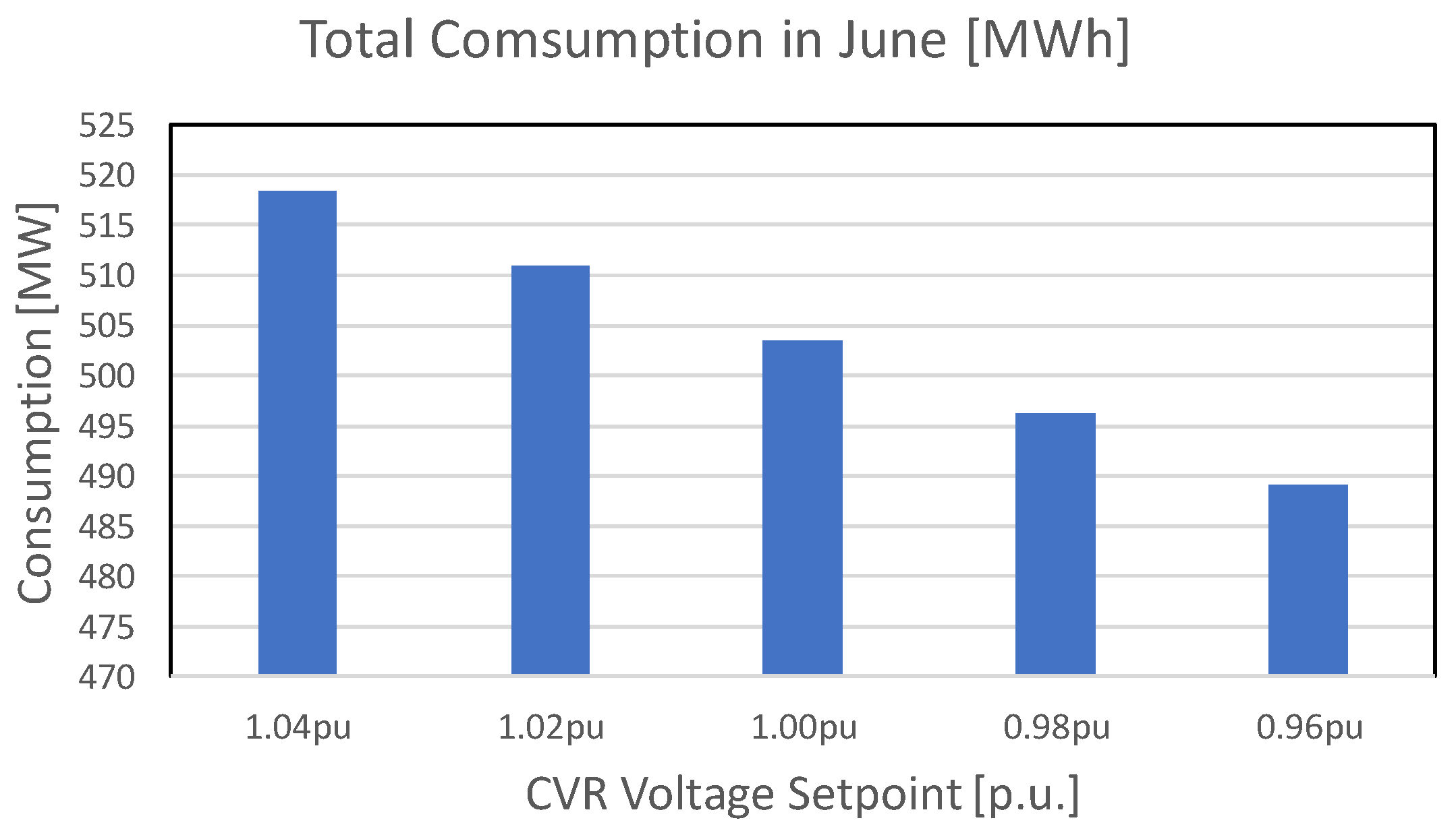
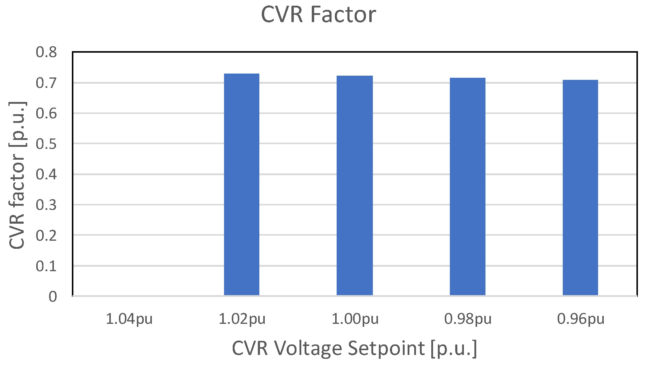
A quantitative evaluation of these energy losses for the month of June is depicted in Figure 7, which clearly demonstrates the potential savings in energy consumed as CVR is employed. With this information in hand, the CVRfactor, calculated by using (3), can be assessed for this feeder in June. This is shown in Figure 8, which expectedly suggests that the CVR factor itself is somewhat constant for different CVR setpoints.
4.3. The Impact of Inverter Operation Mode on PV Production
The effect of CVR on PV production was simulated for the various inverter operating modes. For this analysis, two Volt-Watt modes were investigated. This is because the factory default Volt-Watt does not curtail production entirely until the voltage reaches 115% of nominal, which is well in excess of the default overvoltage trip settings of 110%. This is shown in Figure 9. Instead, this work proposes a more conservative curtailment strategy, where the entire production is curtailed at 108%, which, in the case of very high DER penetration (such as in the case study of this paper), results in overall, system-wide reduced inverter trips, as the majority of the DERs will share the necessary curtailment to avoid inverters tripping in the system. The figure shows both the factory default Volt-Watt curve (termed as VW–Default) as well as the proposed Volt-Watt curve (termed as VW–Custom).
This study also shows the adopted Volt-VAR curve, which is the inverter factory default behavior and is shown in Figure 10. This curve reveals that the inverters will reach their maximum reactive power exchange at the point the voltage deviates at ± 5%, leading the inverter to its maximum under-excitation when voltage is at 105%. To note, as per IEEE 1547 [5], the maximum reactive power exchange is 44% of the inverter rating.
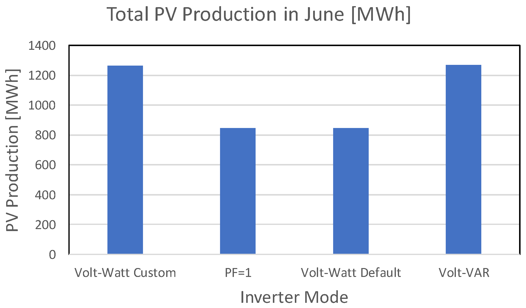
The results of the system-wide PV energy production for the month of June is shown in Figure 11 for the various inverter operating modes. To obtain the results shown in this section, an hourly load flow was conducted, and at each time step, the voltage control curves presented above were simulated in each inverter. The active and reactive power output of each inverter was monitored and stored, as well as the active and reactive power consumed by each load in the system. Line active power losses were also calculated and stored. In this study, every time the voltage reached 110% at an inverter terminal, the inverter trip was simulated in that the inverter was disconnected from the system for 15 mins and reconnected after this time delay. This choice was made because, as per [5], inverters must wait for system voltage and frequency to be stable for a configurable amount of time (which can be configured between 1 and 15 mins) before reconnecting to the grid. With this strategy, Figure 11 reveals the following:
- -
- The operating modes that result in most production are the customized Volt-Watt modes and the Volt-VAR modes.
- -
- The customized Volt-Watt mode and the Volt-VAR modes result in the least amount of inverter trips. As a matter of fact, the customized Volt-Watt mode did not result in a single trip, as all inverters will completely cease export before reaching 110%. The Volt-VAR resulted in very few hours where an inverter would trip.
- -
- Surprisingly, the default Volt-Watt mode results in very high curtailment because its setpoints allow for inverter tripping, which in very sunny days results in a lot of inverter off-time.
- -
- As expected, the constant power factor mode (set at 100%) results in the least overall production, as it results in the most amount of inverter off-time due to trips.
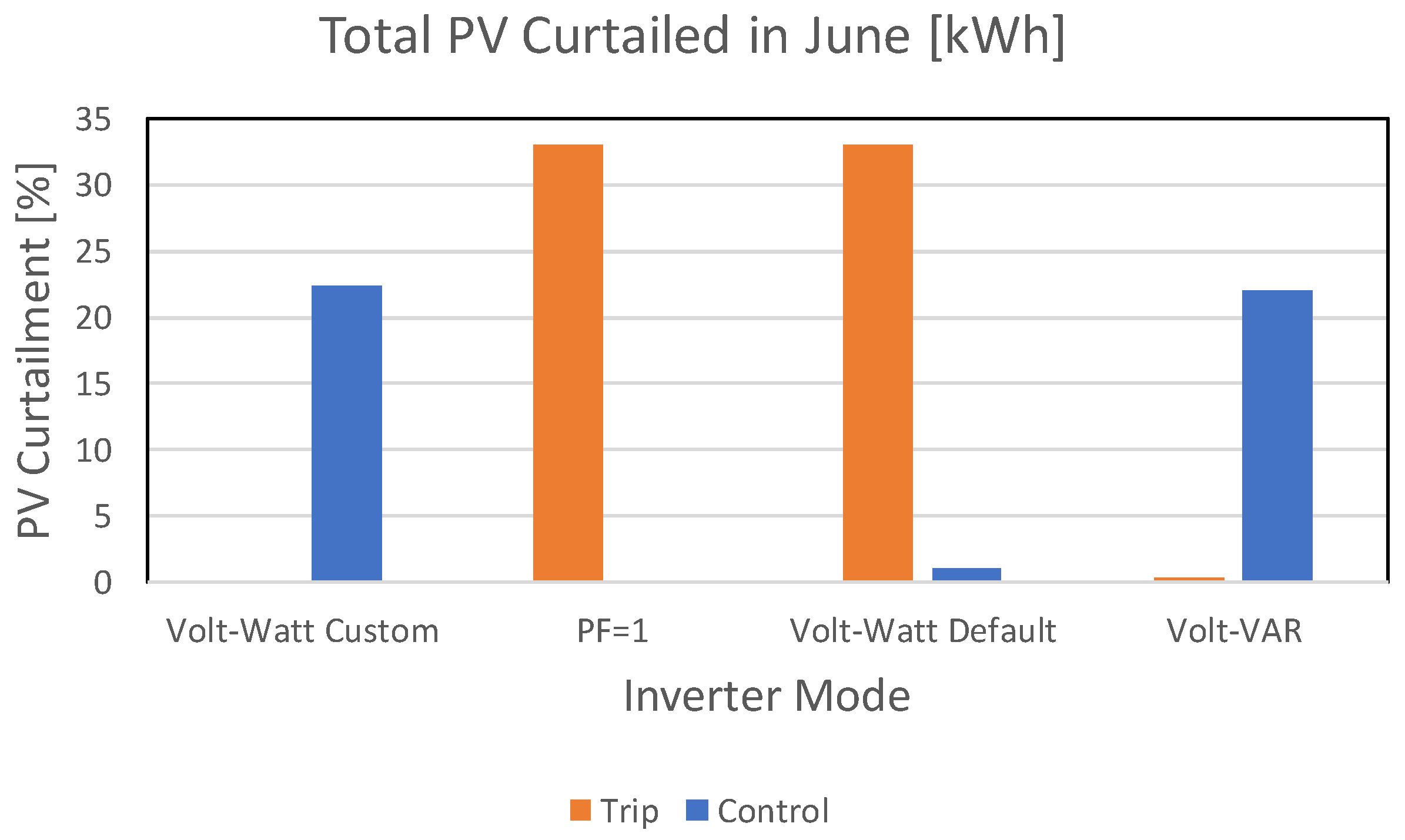
Figure 12 displays how the trips influence production. The findings from this figure are:
- -
- The custom Volt-Watt mode does not result in any trip, and its entire curtailment is due to controlled inverter output.
- -
- The constant power factor mode has the highest curtailment, which is entirely a result of inverter trips and none is controlled.
- -
- The default Volt-Watt mode, surprisingly, results in more off-time due to trips than to controlled power output. This is primarily due to the solar irradiation pattern of this area in June. This northern Canadian city has extremely sunny summer days with very low cloud and precipitation (PV pattern will be discussed in the next subsection).
- -
- The Volt-VAR curve results in very few inverter trips, and its curtailment is almost entirely controlled by the inverter.
4.4. The Impact of CVR on the PV Production
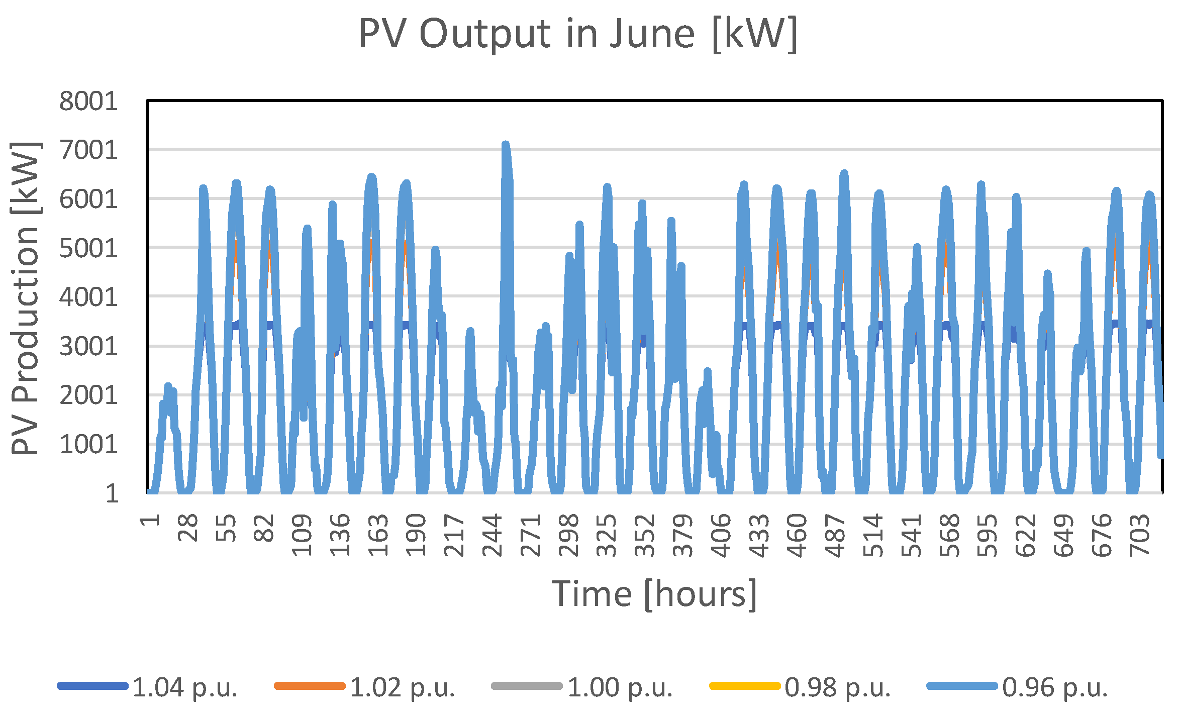
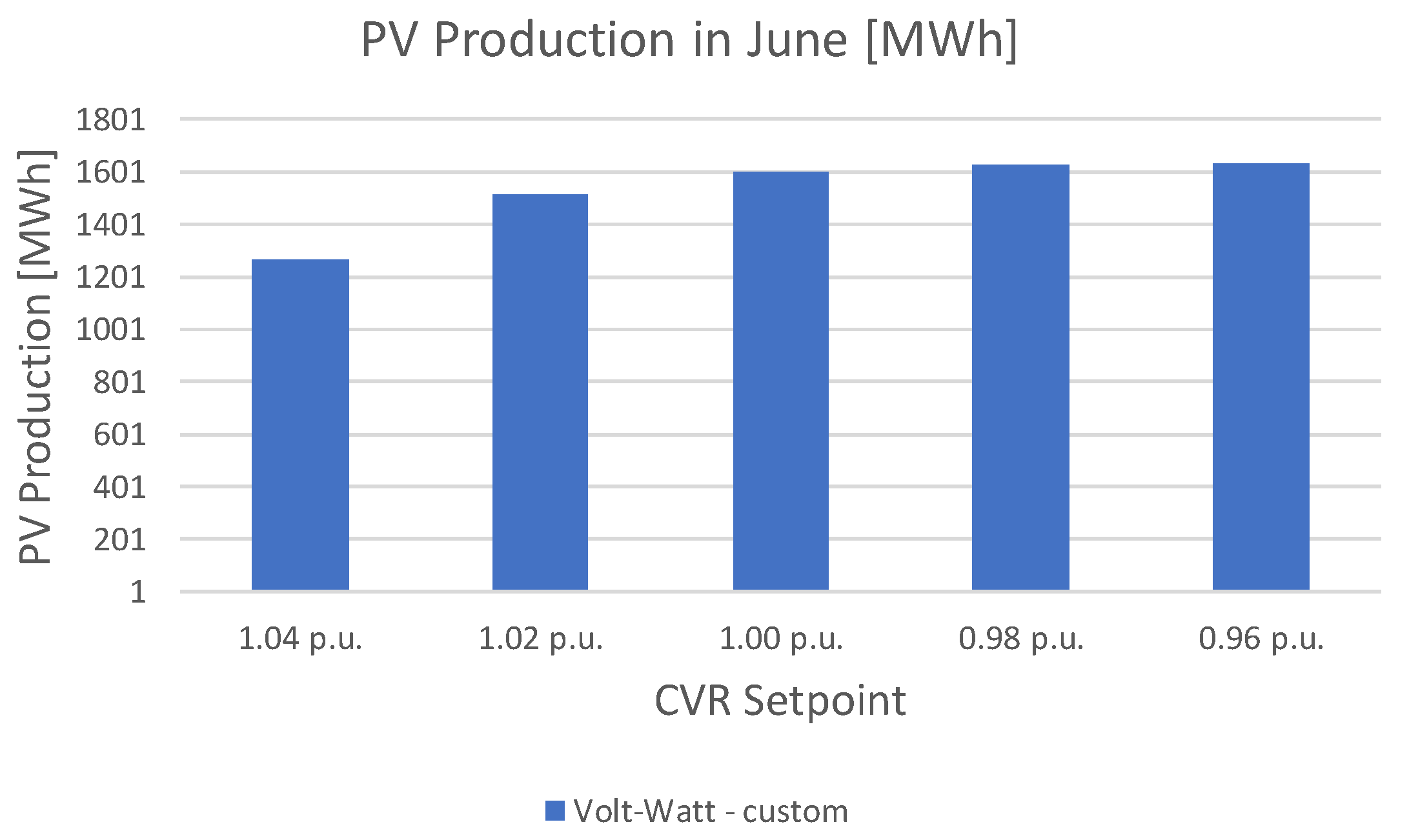
The effect of CVR on PV production was evaluated for the system. First, different setpoints for the CVR were employed to control voltage at the customer that experienced the lowest voltage along the feeder. Different setpoints, namely 1.04 p.u., 1.02 p.u., 1.00 p.u., 0.98 p.u., and 0.96 p.u., as seen at the distribution primary (in this system, the 25 kV), were investigated. To note, these comprise the entire planning target voltage range. For conciseness, this subsection only shows the results of the customized Volt-Watt mode. This is displayed in Figure 13, which shows the PV production pattern for the month of June. As in the past section, a time-series hourly load flow was carried out and the active and reactive power flows were stored for further analysis. Among other observations, it is possible to infer that the solar irradiation ramp rates are steep, resulting in inverter output rising accordingly. It is notable that higher voltage setpoints result in visible curtailment. Figure 14 summarizes the entire energy produced for these different CVR setpoints. As expected, the lower the voltage setpoint, the more production takes place, as there is much less curtailment at a lower voltage.
4.5. The Impact of Load Composition on PV Production
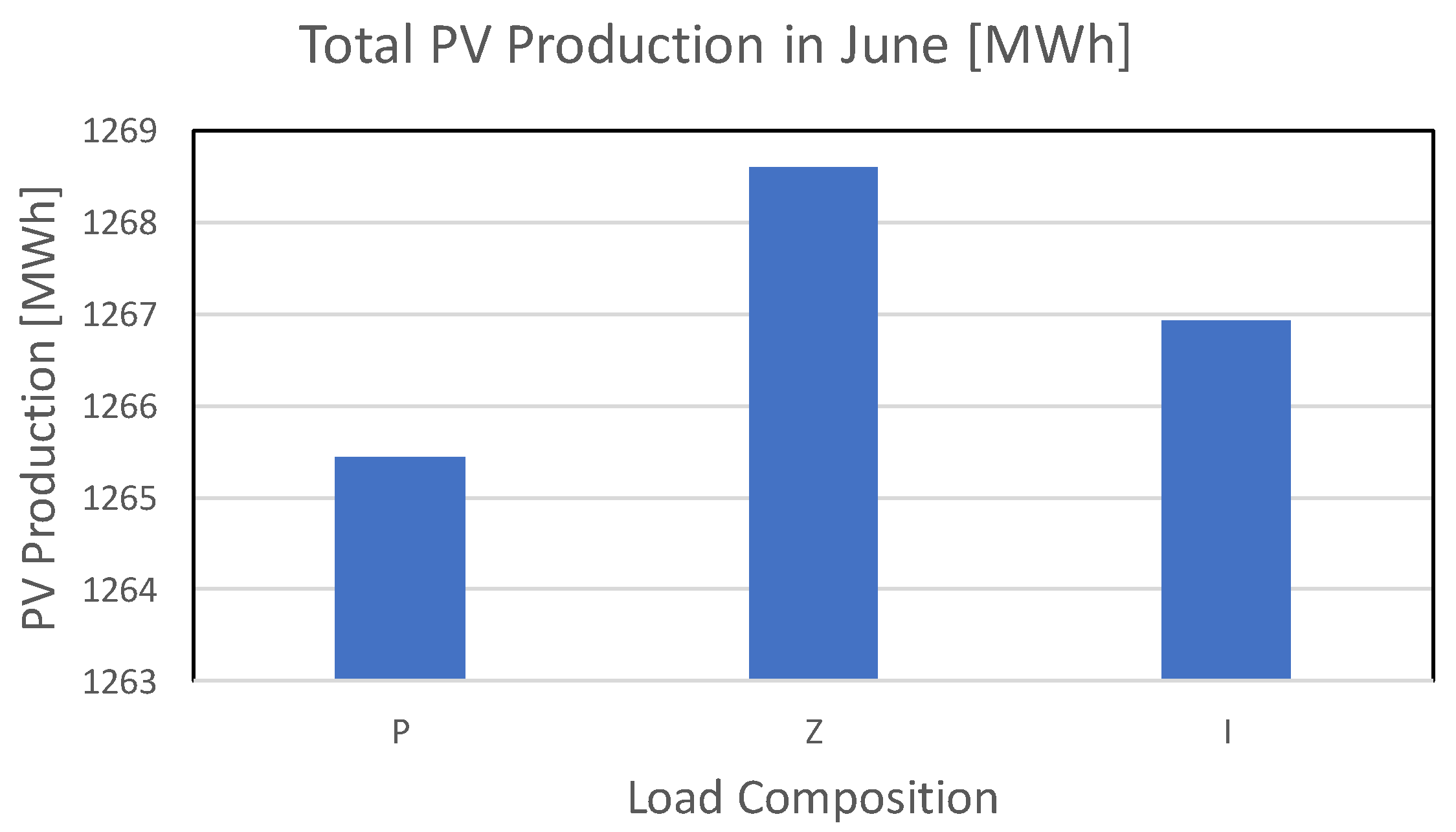
Lastly, the impact of system load composition on PV production is analyzed and shown in Figure 15. This figure reveals greater production results for the constant impedance load, and lower results for the constant power load. This is expected, because a constant impedance load draws more power from the grid, and consequently from the distributed PV generators, for voltages higher than 1.p.u., which results in higher power absorbed (proportional to the square of the applied terminal voltage). Conversely, constant power loads draw a constant amount of power regardless of the applied terminal voltage. Lastly, constant current loads are in between, with power absorbed rising with voltages above 1 p.u., proportional to the applied terminal voltage.
4.6. The Impact of PV Generation on Energy Savings
In this subsection, the load was modeled as 50% constant power and 50% constant impedance. Like in previous subsections, it is also assumed the PV penetration reaches 50% of feeder peak load.
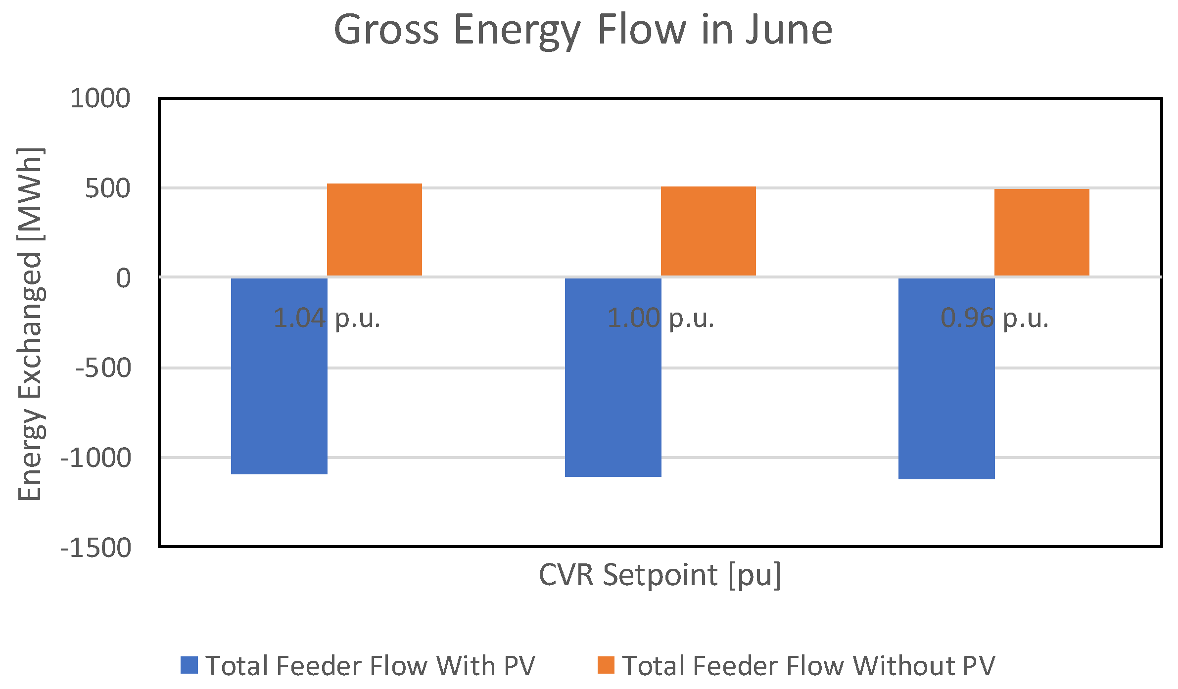
The mass deployment of renewable generation reduces the amount of energy consumed by the aggregated load in the feeder. This is shown in Figure 16, which shows the total feeder energy transacted in June for the baseline case (without DERs, the right-hand side bar in each of the three results) and for the case with high DER penetration (the left-hand side bar in each of the three results). Each of the three results corresponds to a CVR setpoint, namely 1.04 p.u., 1.00 p.u., and 0.96 p.u. of voltage sensed at the lowest voltage point of the feeder. As expected, this feeder with high PV generation penetration results in net export at the feeder level over the billing cycle, since the month of June is very sunny. Conversely, the masked load, which is shown as the baseline, presents itself a net import. In this figure, it is difficult to observe the effect of CVR, because it has small impact as compared to overall consumption and/or production and is better visualized in subsequent figures.
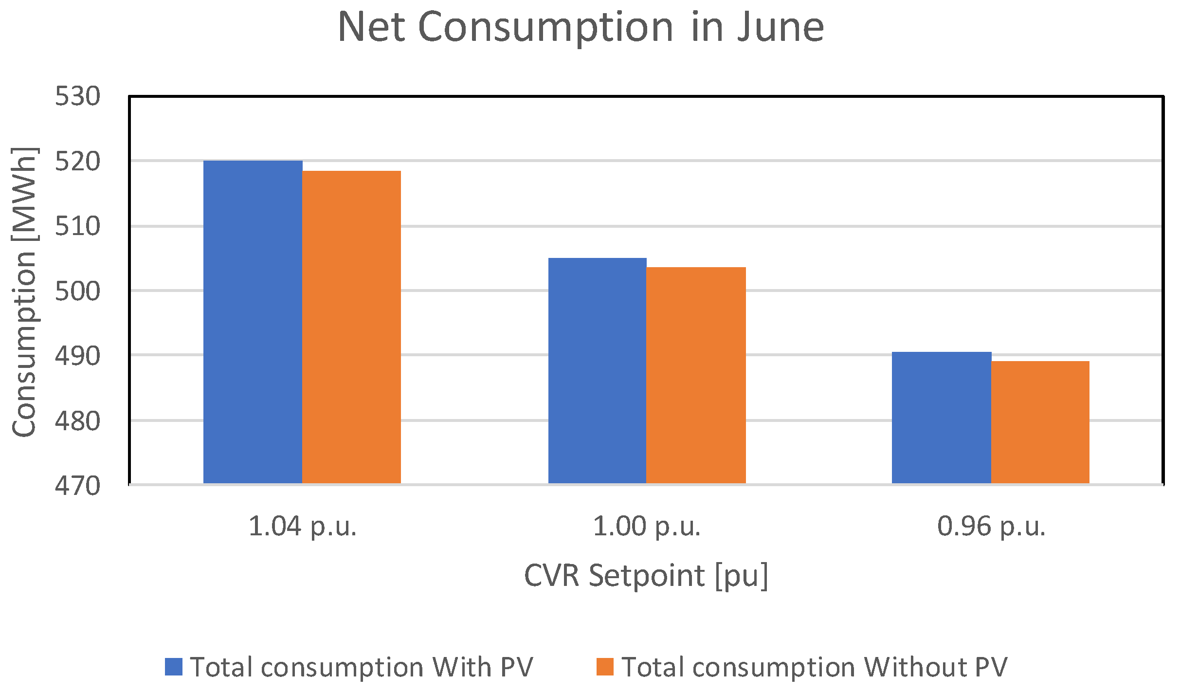
The total energy consumed by the load aggregation is shown in Figure 17, which shows the totalized consumption of all loads in the feeder, calculated by adding up all of the loads’ hourly demand over the month of June to obtain the energy. This result confirms CVR can reduce load consumption, but also that the consumption is higher with PV. This high PV penetration results in slightly elevated voltage, as discussed in the previous subsections. As a result, higher PV penetration reduces the effectiveness of CVR. This is expected. However, the high PV penetration is not high enough to counter the effect of CVR entirely. As in the previous cases, the CVRfactor was calculated as being around 0.7, and is omitted from the paper to save space.
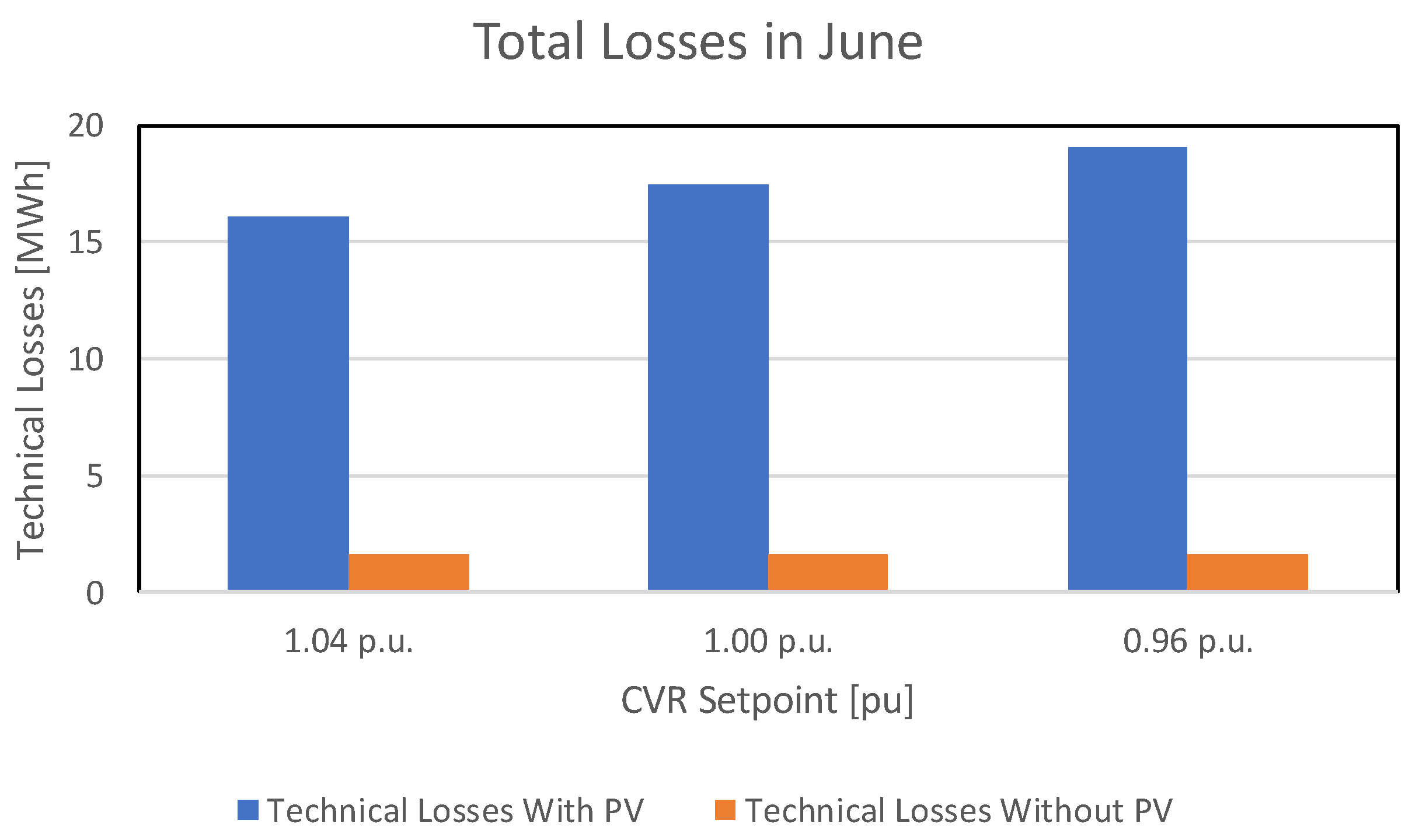
Lastly, total technical losses (RI2) are quantified in Figure 18. These are calculated by adding up the hourly energy flows on every piece of conductor contained in the feeder. As expected, the CVR increases technical losses. Interestingly, the high PV penetration increases the technical losses because, in June, the PV generation exceeds the load by a large amount and power is predominantly flowing in reverse (in this northern city, sunlight times exceed 15 h per day). In winter, however, where PV only slightly offsets load, it would result in larger savings due to small voltage support.
5. Findings and Concluding Remarks
This paper analyzed the interaction between two grid modernization initiatives, the application of Conservation Voltage Reduction, and the mass adoption of DERs. As identified by many researchers in the past, these two have meaningful interactions with one another. The focus of the paper was during sunlight hours of a northern Canadian city, which experiences very long sunny days in June. These results are interesting as not all are intuitive.
The main finding of the paper, however, is that even with very large PV penetration in the sunniest month, the effect of CVR is not countered and it can still be used to achieve significant energy savings with CVRfactor approaching 70%. Other general observations, useful for distribution planning, are highlighted below:
- For locations that have steep solar irradiance ramp rates and very high PV inverter penetration, the Volt-Watt settings that come as factory defaults of most commercial inverters help manage PV output, but do not prevent inverter cessation to energize because total output is not curtailed until voltage reaches 115%, well beyond the factory trip (total cessation) of 110%. It is recommended that utilities create customized Volt-Watt curves to avoid violation to ANSI standards.
- A customized Volt-Watt curve was shown to be the most effective means to manage voltage both at the distribution primary and secondary. This results in controllable curtailment, rather than uncontrolled trips (cease to energize).
- The employment of CVR results in increased hosting capacity. This PV generation penetration reduces the effectiveness of CVR, but only by a small amount.
- Volt-VAR can be very effective, but does not prevent inverter cessation to energize either, as VAR limits are reached quickly (as demonstrated in Equation (2)) and inverters must cease to energize once voltage reaches 110%.
- The default mode of constant power factor operation at 100%, which traditionally was the mode prescribed by most utilities, results in very substantial inverter cessation to energize, due to voltage rises, and, subsequently, substantial energy curtailed uncontrollably.
Author Contributions
Conceptualization, A.B.N.; Data curation, M.D.; Formal analysis, A.B.N.; Software, A.B.N.; Visualization, M.D.; Writing—original draft, A.B.N.; Writing—review & editing, A.B.N. All authors have read and agreed to the published version of the manuscript.
Funding
This research received no external funding.
Conflicts of Interest
The authors declare no conflict of interest
References
- Dugan, R.; McDermott, T. Operating Conflicts for Distributed Generation on Distribution Systems. In Proceedings of the IEEE 2001 Rural Electric Power Conference, Little Rock, AR, USA, 29 April–1 May 2001. [Google Scholar]
- Dugan, R. Distributed Generation. IEEE Ind. Appl. Magaz. 2002, 8, 19–25. [Google Scholar] [CrossRef]
- Available online: http://www.cpuc.ca.gov/Rule21/ (accessed on 14 September 2020).
- Underwriters Laboratories. Underwriters Laboratories UL 1741 Supplement A; Underwriters Laboratories: Northbrook, IL, USA, 2010. [Google Scholar]
- Photovoltaics, D.G.; Storage, E. IEEE Standard for Interconnection and Interoperability of Distributed Energy Resources with Associated Electric Power Systems Interfaces. IEEE Std 2018, 1547–2018. [Google Scholar] [CrossRef]
- CSA Group. CAN/CSA-C22.3 NO. 9-20—Interconnection of Distributed Resources and Electricity Supply Systems; CSA Group: Toronto, ON, Canada, 2020. [Google Scholar]
- 1547.1-2020: IEEE Standard Conformance Test Procedures for Equipment Interconnecting Distributed Energy Resources with Electric Power Systems and Associated Interfaces. IEEE Std 2020. [CrossRef]
- Scalley, B.R.; Kasten, D.G. The Effects of Distribution Voltage Reduction on Power and Energy Consumption. IEEE Trans. Edu. 1981, 24, 210–216. [Google Scholar] [CrossRef]
- Kirshner, D. Implementation of conservation voltage reduction at Commonwealth Edison. IEEE Trans. Power Syst. 1990, 5, 1178–1182. [Google Scholar] [CrossRef]
- Singh, R.; Tuffner, F.; Fuller, J.; Schneider, K. Effects of distributed energy resources on conservation voltage reduction (CVR). In Proceedings of the 2011 IEEE Power and Energy Society General Meeting, Detroit, MI, USA, 24–28 July 2011; pp. 1–7. [Google Scholar]
- Lawanson, T.; Karandeh, R.; Cecchi, V.; Kling, A. Impacts of Distributed Energy Resources and Load Models on Conservation Voltage Reduction. In Proceedings of the 2018 Clemson University Power Systems Conference (PSC), Charleston, SC, USA, 4–7 September 2018; pp. 1–6. [Google Scholar]
- Bokhari, A.; Raza, A.; Diaz-Aguiló, M.; De Leon, F.; Czarkowski, D.; Uosef, R.E.; Wang, D. Combined Effect of CVR and DG Penetration in the Voltage Profile of Low-Voltage Secondary Distribution Networks. IEEE Trans. Power Deliv. 2016, 31, 286–293. [Google Scholar]
- Zhang, Y.; Gatsis, N.; Giannakis, G.B. Robust Energy Management for Microgrids with High-Penetration Renewables. IEEE Trans. Sustain. Energy 2013, 4, 944–953. [Google Scholar] [CrossRef] [Green Version]
- Carli, R.; Dotoli, M.; Jantzen, J.; Kristensen, M.; Othman, S.B. Energy scheduling of a smart microgrid with shared photovoltaic panels and storage: The case of the Ballen marina in Samsø. Energy 2020, 198, 117188. [Google Scholar] [CrossRef]
- Masters, C.L. Voltage Rise—The Big Issue when Connecting Embedded Generation to Long 11 kV Overhead Lines. IEEE Power Eng. J. 2002, 16, 5–12. [Google Scholar] [CrossRef]
- Wilson, T.L. Energy conservation with voltage reduction-fact or fantasy. In Proceedings of the 2002 Rural Electric Power Conference, Colorado Springs, CO, USA, 5–7 May 2002; p. C3-1. [Google Scholar]
- CSA Group. CSA C235:2019, Preferred Voltage Levels for AC Systems up to 50 000 V; CSA Group: Toronto, ON, Canada, 2019. [Google Scholar]
Figure 1.
System used to illustrate the issue of voltage rise.

Figure 2.
Generic Smart Inverter voltage-reactive power (Volt-VAR) Characteristics.

Figure 3.
Generic Smart Inverter voltage-active power (Volt-Watt) Characteristic.

Figure 4.
Simplified illustration of the feeder under analysis.

Figure 5.
Total downstream losses in June for different conservation voltage reduction (CVR) setpoints on an hourly basis.
Figure 5.
Total downstream losses in June for different conservation voltage reduction (CVR) setpoints on an hourly basis.

Figure 6.
Total load consumption in June for different CVR setpoints on an hourly basis.

Figure 7.
Total energy consumed in June for different CVR setpoints.

Figure 8.
CVR Factor in June for different setpoints.

Figure 9.
Volt-Watt curves used in this study (Default and Custom).

Figure 10.
Volt-VAR curve used in this study (inverter default factory curve).

Figure 11.
Total photovoltaic (PV) energy produced in June for different inverter modes.

Figure 12.
Total PV curtailed in June due to inverter trips and control.

Figure 13.
PV production time series for various CVR voltage setpoints.

Figure 14.
Total PV produced in June for various CVR voltage setpoints.

Figure 15.
Effect of load composition on energy produced in June.

Figure 16.
Energy transacted in the billing cycle comparing the case of large-scale PV penetration and that without (masked load only).
Figure 16.
Energy transacted in the billing cycle comparing the case of large-scale PV penetration and that without (masked load only).

Figure 17.
Effect of PV on energy consumed in June for different CVR setpoints.

Figure 18.
Effect of PV on technical losses in June for different CVR setpoints.

© 2020 by the authors. Licensee MDPI, Basel, Switzerland. This article is an open access article distributed under the terms and conditions of the Creative Commons Attribution (CC BY) license (http://creativecommons.org/licenses/by/4.0/).
Share and Cite
MDPI and ACS Style
Nassif, A.B.; Dong, M. Characterizing the Effect of Conservation Voltage Reduction on the Hosting Capacity of Inverter-Based Distributed Energy Resources. Electronics 2020, 9, 1517. https://doi.org/10.3390/electronics9091517
AMA Style
Nassif AB, Dong M. Characterizing the Effect of Conservation Voltage Reduction on the Hosting Capacity of Inverter-Based Distributed Energy Resources. Electronics. 2020; 9(9):1517. https://doi.org/10.3390/electronics9091517
Chicago/Turabian StyleNassif, Alexandre B., and Ming Dong. 2020. "Characterizing the Effect of Conservation Voltage Reduction on the Hosting Capacity of Inverter-Based Distributed Energy Resources" Electronics 9, no. 9: 1517. https://doi.org/10.3390/electronics9091517
Note that from the first issue of 2016, this journal uses article numbers instead of page numbers. See further details here.