Experimental Analysis of a Novel Double Damper System with Semi-Active Control

Abstract

An experimental study was conducted to compare the performance of an in-house built novel double semi-active damper against a conventional semi-active single damper. Different performance metrics were analyzed, and the performance of the two dampers was evaluated based on these metrics. A Hybrid Skyhook–Groundhook control algorithm was developed and implemented on the variable orifice double damper. The semi-active single damper is governed via two separate control strategies, namely—Skyhook and Groundhook control, respectively. The effectiveness of each algorithm is better understood by adding a normal load on top of the Shock Dyno, thus modifying it to act as a quarter car test rig. The sprung and unsprung acceleration data are collected via the accelerometers mounted on the Shock Dyno through a Data Acquisition System. The results obtained from this experiment provide a strong basis that the semi-active double damper performs better in terms of the comfort cost than that of the commercial semi-active single dampers.

1. Introduction

The automotive suspension system plays a crucial role in maintaining the vehicle dynamics of the car for changes in road input and variations in the normal weight distribution. An effective suspension system ensures passenger ride comfort for unpredictable input variations, and allows a sufficient amount of tire-road contact for proper road handling. Damper design and analysis is the most pivotal part when analyzing any suspension system. There are three commonly used suspension systems-passive, semi-active, and active suspensions with each one having its advantages and limitations over the other. Conventional passive suspension systems come with the inherent limitation that they cannot cater to both road-holding and ride comfort at the same time. For example, a soft suspension system may be better at providing ride comfort but will not perform as well in handling as compared to a harder, stiffer suspension and vice-versa [1]. A numerical simulation study conducted by Sharp and Hassan [2] also shows that for obtaining the best performance from any particular type of suspension for a spectrum of different operating conditions such as road undulations, vehicle speed variations, and fixed working space, requires the adjustment of suspension parameters through wide ranges.

Active suspension systems change the damping coefficient of the vehicle suspension by applying a force with the help of hydraulic or electric actuators [3]. These controlled forces help in modifying the ride and handling characteristics at every instant in real-time. A study performed by Xue et al. [4] has shown the comparison between the four different configurations of suspensions systems-passive, semi-active, hydraulic, or pneumatic active and electromagnetic active. They concluded that even though the hydraulic active suspensions systems have slightly better ride comfort and handling characteristics, it comes with inherent drawbacks of having a complex structure and a very high cost. Along with this, the use of different control algorithms for semi-active dampers has increased their reliability over the active suspension systems. These advantages of semi-active dampers have justified their use for commercial vehicle applications [5,6,7].

Semi-active suspension systems lie between passive and active in terms of performance, cost, and complexity. They can vary the damping characteristics by either using a variable orifice [8] or variable viscosity fluids [9,10]. Variable orifice semi-active suspension systems use a position control valve to adjust the orifice area through which the damper fluid flows [11]. This variation in orifice area is directly proportional to the damping coefficient, which in turn varies the force transmitted to the vehicle chassis. Variable fluid viscosity semi-active dampers, on the other hand, make use of Electrorheological (ER) and Magnetorheological (MR) fluids to vary the damping force. When subjected to a magnetic field, the MR fluids change their properties and act as a semi-solid material, thus altering the damping properties of the damper [12].

Sabino et al. [13] used a Magne-Ride Delphi damper, which is an MR damper for testing three specific control algorithms; on-off Skyhook control, continuous Skyhook control and Skyhook algorithm based fuzzy logic control. However, these MR dampers have inherent limitations of particle settling within the damper, causing abrasions. These abrasions along the inner wall of the damper may lead to wearing damper material resulting in decreased life.

Peng et al. [14] also made use of MR dampers for semi-active suspension control using Skyhook Control. They used a B class vehicle and replaced the conventional four hydraulic dampers with MR dampers and utilized eight accelerometers—four for sprung and four for unsprung mass accelerations. They were able to reduce the peak vertical acceleration of the driver’s seat to 0.32 g. Tang et al. [15] developed a state-observer based fuzzy controller for a MR damper. The validation of the algorithm was done on a quarter car test rig which had provisions for collecting the sprung and unsprung mass acceleration data.

Krauze et al. [16], along with using accelerometers, also made use of Linear Variable Differential Transformer (LVDT) for measuring the vertical deflection of the suspension on an instrumented All-Terrain Vehicle. They used a sampling frequency of 500 Hz and frequency of excitation between 1.5–12 Hz. An important conclusion derived was that accelerometer-based velocity estimation gave better results for Skyhook Control, whereas, the Groundhook control performed better with LVDT based measurement methods. Gong and Chen [17] implemented variable damping control strategy on a variable orifice damper. They essentially made use of displacement sensors as a feedback unit upon which the variable damping control strategy was based. A reduction in the body, roll and pitch angle accelerations were found in comparison with a passive damper.

In this paper, the application of a Hybrid Skyhook–Groundhook control algorithm is proposed to be implemented experimentally on a novel damper design, called “Double Damper”.

1.1. Double Damper

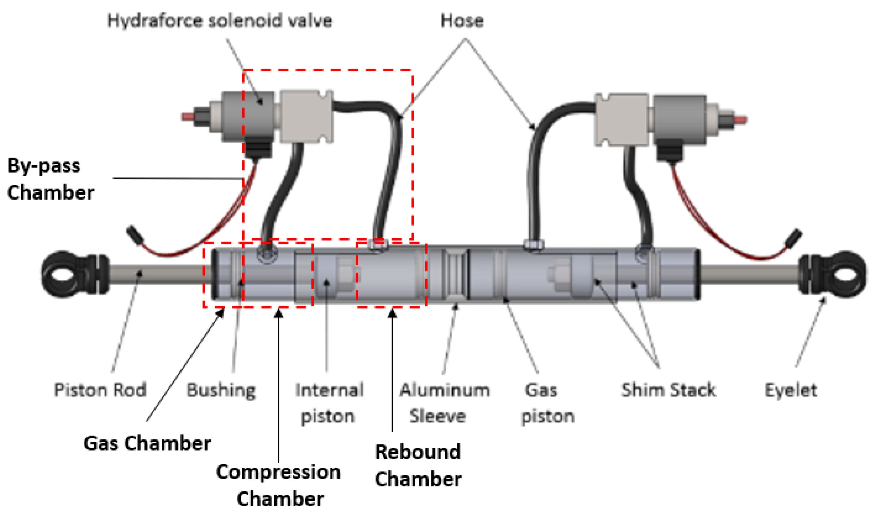
A Double Damper (Figure 1) consists of two controllable dampers placed in series and was used for carrying out the experiments. Tyagi [18] designed, developed, and manufactured this damper in-house at the Center for Tire Research (CenTire). The internal construction of the double damper is as shown in Figure 2. The damper consists of 4 main chambers—compression, rebound, gas, and by-pass, respectively. The gas chamber is at the top of the tube, and it is separated from the compression chamber by a floating piston. This piston separates the nitrogen in the gas chamber from the oil in the compression chamber. The compression chamber sits between the floating piston of the gas chamber and the piston. On the other side of the piston and opposite to the compression chamber is the rebound chamber. The rebound chamber is connected to the piston of the damper by a rod. Also, it is connected to the compression chamber throw the by-pass valve. These by-pass valves are essentially solenoid valves, one for each damper. These valves control the flow rate of oil passing from the compression chamber to the rebound chamber for each individual damper. The damper was modeled, taking into account pressure and flow variations within the damper. The damper, as shown in Figure 1 has two controllable by-pass valves. Figure 2 illustrates different part of the double-damper.

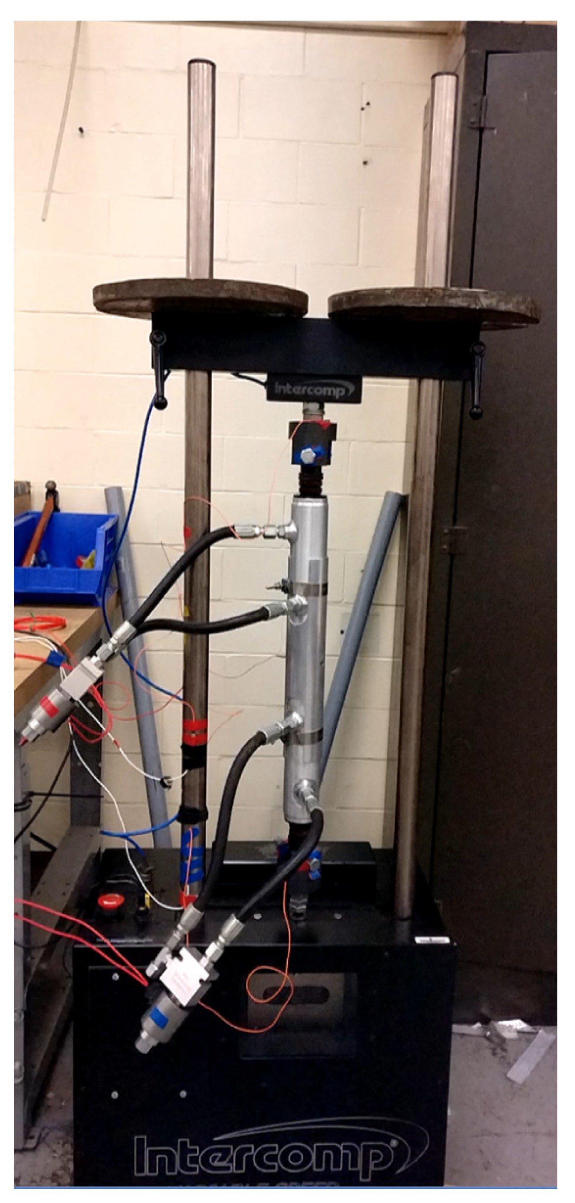
For experimentation, a set of two springs is attached in parallel to the double damper. These springs correspond to the typical configuration of mounting a shock absorber in a vehicle. For the single damper, due to geometrical constraints, a single spring is attached in parallel to this damper. The spring attached in parallel with the single damper has a stiffness coefficient equivalent to the combined stiffness of the two springs in parallel with the double damper. The entire setup consisting of the double damper and springs mounted on the Shock Dyno can be seen in Figure 3.

This study’s primary goal is to develop and implement a control algorithm for controlling the damping coefficient of the double damper based on the relative velocity difference between the sprung and unsprung mass in real-time. A dedicated experimental setup was developed for evaluating the performance of the semi-active double damper for different operating conditions. The control algorithm and its implementation for the double-damper are explained in the subsequent sections. Later results were compared to a semi-active single as a benchmark to evaluate the performance of the double-damper.

In order to evaluate the performance of dampers, a metric called ’Comfort cost’ is compared. Comfort cost can be essentially looked at as the extent of comfort a particular ride can offer on undulated topography. This cost is implemented by calculating the spectral power of the sprung mass acceleration data, in the low frequency range. The power of a signal in low frequency zone corresponds to the extent of comfort a damper can provide. Since the human comfort is associated with lower frequencies, this range is looked for evaluating comfort cost. Similarly, the spectral energy content of data at high frequencies is seen for evaluating the road holding property of the vehicle as the tire hop frequency is comparatively higher. A low spectral energy content in the low frequency zone corresponds to a smoother ride as the sprung mass resonances are more damped. Since the resonances are damper, it essentially leads to a less area under the curve in the spectral domain, and hence smaller power spectral density. With respect to these properties, comfort cost is chosen for evaluating the ride comfort offered by different dampers.

1.1.1. Control Algorithms

Different control strategies were implemented to minimize the vertical acceleration of the sprung mass and to improve the road-holding capabilities by varying the orifice area of the solenoid valves [19,20,21]. Since we are using a Double Damper, we have developed a hybrid control algorithm that employs Groundhook control on the lower damper and Skyhook control on the upper damper [22]. This algorithm was developed on MATLAB/Simulink and effectively deployed on the valves mounted on the Double Damper.

1.1.2. Hybrid Skyhook–Groundhook Control

Valášek et al. [22] performed an in-depth study on the combination of Groundhook and Skyhook control strategy for semi-active suspension systems mainly for trucks. In the case of the double-damper, the Groundhook control algorithm is implemented on the lower damper to ensure better road handling characteristics and Skyhook control algorithm on the upper damper. This strategy provides improved ride comfort. This concept of a hybrid control algorithm was reviewed by Goncalves and Ahmadian [23] in which they concluded that such an algorithm reduced the peak to peak displacements and accelerations of both sprung and unsprung masses. A similar simulation study was conducted in [24] which showed the comparison between Skyhook, hybrid and a fuzzy hybrid control algorithm. They also found that the hybrid control algorithm proved to perform better than the individual Skyhook control. The control strategy is based upon the relative velocity difference obtained from three accelerometers mounted on the damper and Shock Dyno mounts. Skyhook control is based on the velocity difference between the double damper (Body Accelerometer) and the sprung mass (Upper Accelerometer) whereas the Groundhook control is based on the velocity difference between the unsprung mass (Lower Accelerometer) and the double damper (Body Accelerometer) as shown in Equation (1).

$$\begin{array}{c}\hfill \dot{x_{upper}}(\dot{x_{upper}}-\dot{x_{body}})\ge 0c_{sky}=c_{max}\\ \hfill \dot{x_{upper}}(\dot{x_{upper}}-\dot{x_{body}})<0c_{sky}=c_{min}\\ \hfill \dot{-x_{lower}}(\dot{x_{body}}-\dot{x_{lower}})\ge 0c_{ground}=c_{max}\\ \hfill \dot{x_{lower}}(\dot{x_{body}}-\dot{x_{lower}})<0c_{ground}=c_{min}\end{array}$$

(1)

where

$\dot{x_{upper}}$: Sprung mass velocity

$\dot{x_{body}}$: Double damper velocity

$\dot{x_{lower}}$: Unsprung mass velocity

$c_{sky}$: Upper damping coefficient

$c_{ground}$: Lower damping coefficient

2. Experimental Setup

This section covers the complete system hardware of the system along with the description of each equipment and the overall process flow. Figure 4 shows the experimental setup used for data collection and testing of the damper on the Shock Dyno. Damper testing is carried out on the Shock Dyno covering frequencies from 0.25–3 Hz [25] that helps capture damper effects on yaw, roll, and pitch dynamics of a typical vehicle.

2.1. Apparatus

The experimental setup for testing the performance of the Double Damper system comprises of the components mentioned in

Table 1. Experimental Apparatus.

Component	Quantity	Model
Double Damper	1	Built In-house
Data Acquisition System (DAQ)	1	NI DAQ USB 6225
Signal Conditioner	1	Dytran 4122b
Test Rig	1	Intercomp Variable Speed Shock Dyno
Valve Driver	2	Hydraforce EVDR-0101A
Solenoid Valve	2	Hydraforce SP10-24
USB-TTL-232R Cable	2	FTDI
Single Axis Accelerometer	3	Dytran 3225F1
Oscilloscope	1	Techtronix CDS-200B
DC Power Supply (12 V)	2	-

.

2.1.1. Shock Dyno

An Intercomp Variable Speed Shock Dyno is used for providing the input excitation to the damper system. The parameters of the Shock Dyno are mentioned in

Table 2. Shock Dyno Specifications.

Parameter	Value
Adjustable Stroke	0.0254 m, 0.0381 m, 0.0508 m, 0.05715 m
Load Cell	907 kg
Variable Speed	0.0127–0.4826 m/s

. A load cell mounted on top of the upper eyelet of the damper. This arrangement ensures the measurement of the damper force transmitted to the vehicle chassis. The construction of the Shock Dyno is such that it has a provision of tightening or loosening the top eyelet (sprung mass) of the damper. This provision of loosening the top end is further used for adding different weights on top of the Dyno mimicking the sprung mass. In order to reduce the vibrations at the upper and the lower ends of the Shock Dyno, mounts were specifically designed corresponding to the eyelet dimensions of the dampers.

2.1.2. Accelerometers

Three single-axis accelerometers (Dytran Model 3225F1) are used for obtaining the accelerations at three different points of the Double Damper System. Three mounting points are chosen on the damper and the Shock Dyno, as shown in Figure 5, which correspond to the unsprung, sprung, and the body accelerations. These are further used as inputs to the control algorithms. The primary reasons for choosing these accelerometers were their low sensitivity and wide frequency response. Petro wax is used as an adhesive for securing the accelerometers at their respective positions. The specifications of the accelerometer are mentioned in

Table 3. Single Axis Accelerometer Specifications.

Parameter	Value
Sensitivity	10 mV/g
Frequency Response	1.6–10,000 Hz
Thermal Coefficient of Sensitivity	0.054/°C
Supply Current	2–20 mA
Compliance Voltage	+18 to +30 V

.

2.1.3. Signal Conditioner

A Dytran 4122b signal conditioner is used for providing the required power supply to operate the accelerometers. The inputs to the signal conditioner are the three accelerometers, and the outputs are passed to the Data Acquisition System, which is explained in the subsequent sections. The key specifications of the signal conditioner have been stated in

Table 4. Signal Conditioner Specifications.

Parameter	Value
Amplifier Gain	$\times 1$, $\times 110$, $\times 1100$
Output Voltage Swing	±10 V
Sensor Supply Current Range	2–20 mA

.

2.1.4. Solenoid Valves

Two by-pass valves are mounted on the double damper to control the amount of fluid flow through the damper. van Rensburg et al. [26] focused on modeling the by-pass valve for a semi-active damper from which it was concluded that the involvement of fast-acting dynamics makes it necessary to use valves capable of handling high pressure and flow rates during damper testing. In order to take this into account, a Hydraforce SP10-24 valve is used for controlling the flow rate of oil from the compression end to the rebounding end in the experiment. It is a proportional solenoid-operated, 2-way, spool-type, normally closed, providing bi-directional fluid metering valve. The response time for the valve from fully closed to open fully is approximately 40 ms. It is acceptable to use these experiments since the sample rate chosen for sending the signal to the solenoid valve from the DAQ is 240 Hz. The gas chamber of the double damper is pressurized to an initial value of 1.37 Mpa. The nitrogen gas in the chamber attains the maximum pressure of 3.79 MPa when the damper is subjected to a velocity of 0.3048 m/s, which is the maximum velocity in this study).

The orifice area of the valve can be varied from 0–0.2 in² (0–0.005 m²) thus allowing flow rate of the fluid flow to go upto 0.5 L/s (0.0005 m³). The input to this solenoid valve is given by the digital output port of the DAQ via the valve driver.

2.1.5. Valve Driver

To accurately meter the opening and closing of the solenoid valve, an EVDR-0101A valve driver is used. This driver is a microprocessor-based valve driver mainly used in hydraulic proportional valve applications. It takes inputs from the Data Acquisition System, which drives the output current to the pre-defined ramp rate, enabling accurate and proportional metering control of the solenoid valve. HF-Impulse software is used for calibrating the driver corresponding to the input signal ratings. The valve driver specifications can be seen in

Table 5. EVDR-0101A Driver Specifications.

Parameter	Value
Power Requirements	9–32 VDC
Control Inputs Digital-Frequency	50–10,000 Hz
Control Output Current	50–2000 mA
Control Output PWM	40–400 Hz

.

The valve driver is calibrated using the HF-Impulse software, which enables the user to communicate with the EVDR driver as well as the solenoid valve. It can also be used to visualize the input as well as the control output signal, which will be given to the solenoid valve. The driver is calibrated such that it takes inputs from 0–5 volts and provides a current output for the solenoid valve to go from fully closed (0 A) to fully open (1.2 A) state. The current output of 1.2 A is as per valve specifications.

2.1.6. Data Acquisition System

A NI DAQ USB 6225 is used for collecting the accelerometer data. The analog outputs from all three accelerometers are fed to the analog input ports of the DAQ. A differential connection is used at the input port of the DAQ for connecting the three accelerometers. This sensor output data is then acquired using MATLAB/Simulink.

The specifications of the NI DAQ are mentioned in

Table 6. Data Acquisition System Specifications.

Parameter	Value
Number of channels (Analog Input)	40 differential or 80 single-ended
ADC Resolution (Analog Input)	16 bits
Sample Rate (Analog Input)	250 kS/s (Multi Channel Maximum)
Counters/Timers	2 (32-bit resolution)

.

The sampling frequency was chosen as 240 Hz, which is the real-time limit of the highest sampling rate that could be achieved with the solenoid valve. Also, the ’Asynchronous’ data collection method is used, which ensures that the data acquisition from the device and the simulation happen in parallel enabling quicker simulation time than the synchronous mode. Data from the device is continuously acquired into a FIFO (First In First Out) buffer in parallel as the simulation runs.

3. Experimental Process

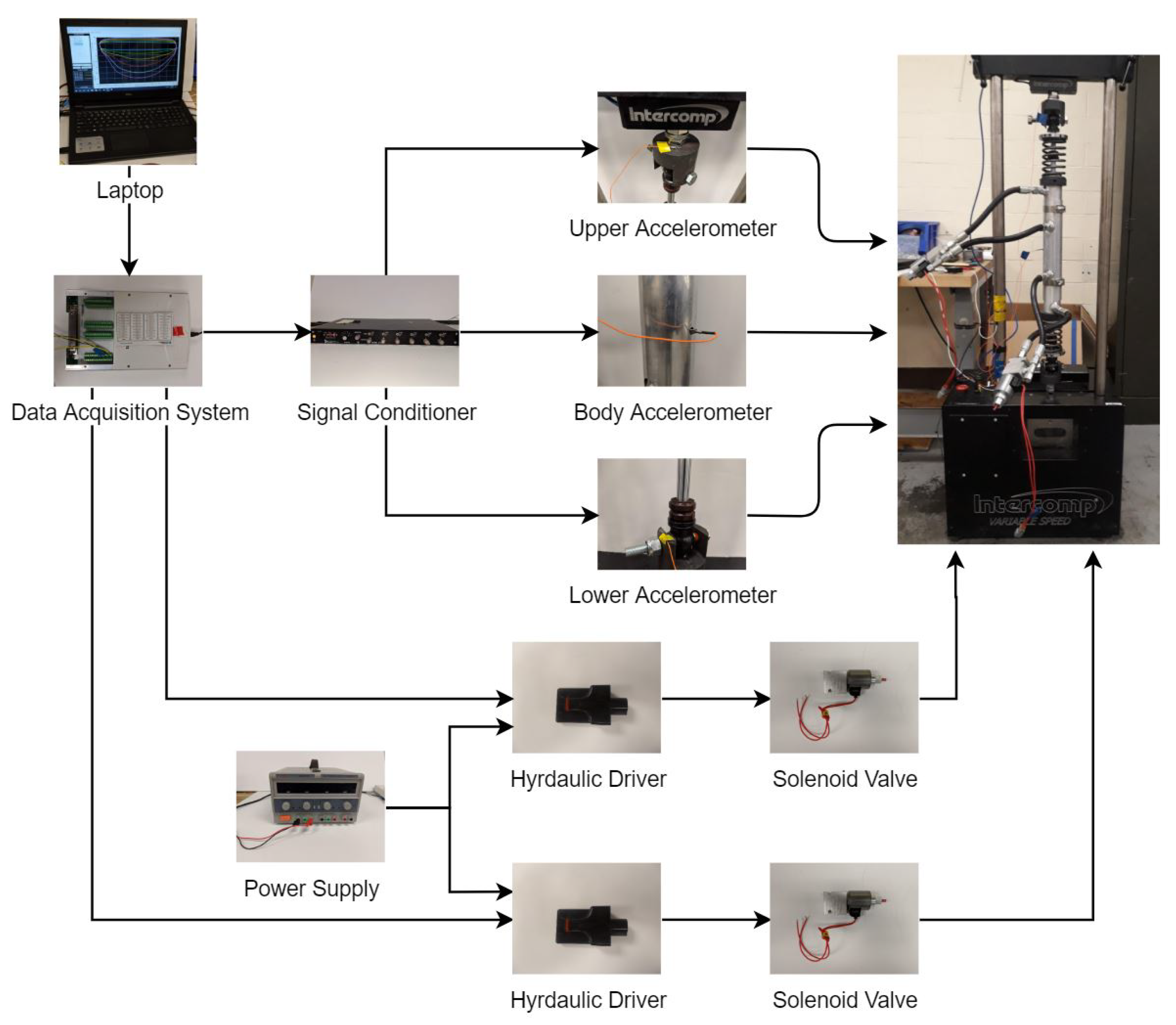
Figure 6 shows the process flow of the experimental setup and the interaction of each hardware with components within the system. Two separate laptops are used—one for operating the Shock Dyno and one for implementing the control algorithms and sending the control signals to the Data Acquisition System. This ensures faster processing for simultaneously running both the Shock Dyno and the control algorithms.

The testing and data collection process for the damper is carried out at different operating conditions to evaluate their effect on the damper performance. These parameters, which are varied during the testing, are explained in the subsequent subsection.

3.1. Loading Conditions

The damper is tested under two types of loading conditions. In the first scenario, the upper mount, on which the damper is mounted, is not free to move. This resembles the conventional damper testing on a Shock Dyno. Due to this kind of loading condition, the Force characteristics of the double damper can be obtained for varying displacement and velocity. For the second scenario, as shown in Figure 7, in order to take into consideration the effect of sprung mass on the damper characteristics, an external load is added on top of the Shock Dyno, and the upper mount is made free to move. This provision also enables the use of control algorithms as the entire control logic is based on the velocity difference of the upper and lower mounting points. The upper limit of the normal load is taken to be 150 lbs (68 kg). This limit is decided based on the gas pressure inside the damper, which is in the order of 1.37 MPa. Exceeding the normal load above 68 kg compresses the damper entirely up to its bottom dead center, and it starts behaving as a rigid body. The lower limit of the normal load is taken as 50 lbs (23 kg) based on the fact that loads less than this have no effect in compressing the piston and the damper starts behaving as a solid body.

3.2. Input Velocity

In order to cover all the road frequencies, the damper is tested with different input velocities. The velocity range is between 8–12 in/s (0.2–0.3 m/s). The upper limit of the velocity is based on the constraint of the Shock Dyno; as above this speed, high-frequency vibrations are induced, resulting in corrupted accelerometer data. At lower velocities, after evaluating the accelerometer data, no significant difference could be found between the sprung and the unsprung accelerations. Hence the lower limit of the velocity was kept at 8 in/s (0.2 m/s).

3.3. Control Algorithm

The semi-active double damper is tested with a Hybrid Skyhook Groundhook control strategy and the single semi-active damper with Skyhook and Groundhook control to measure their ride comfort characteristics. Each control algorithm was modelled in Simulink with identical input parameters.

A brief overview of the testing conditions is summarized in

Table 7. Different operating conditions for Damper Testing.

Normal Load lbs (kg)	Input Velocity in/s (m/s)	Control Algorithm	Damper Type
No Load (Upper Clamp Closed)	8 (0.20)	Hybrid Groundhook Skyhook	Single Damper
50 (22.6)	10 (0.25)	Skyhook	Double Damper
100 (45.35)	12 (0.30)	Groundhook	-

.

4. Signal Processing and Data Analysis

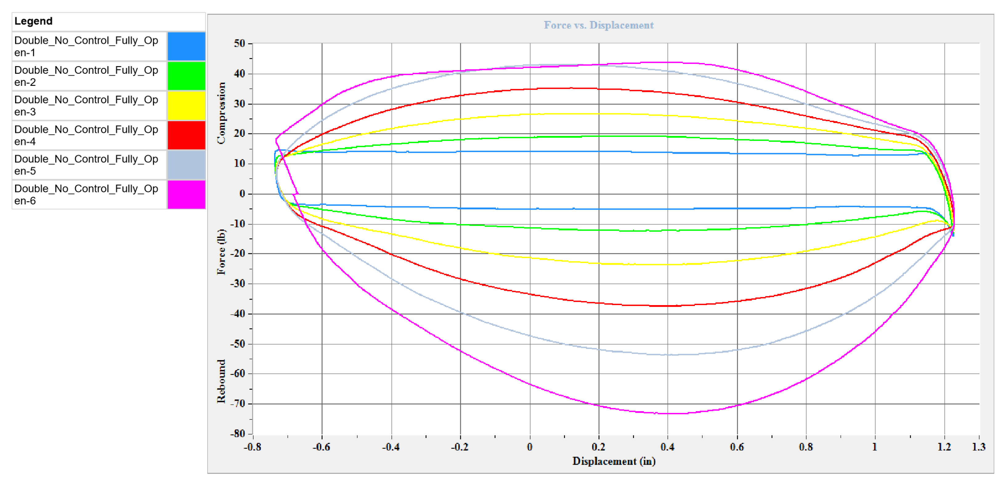
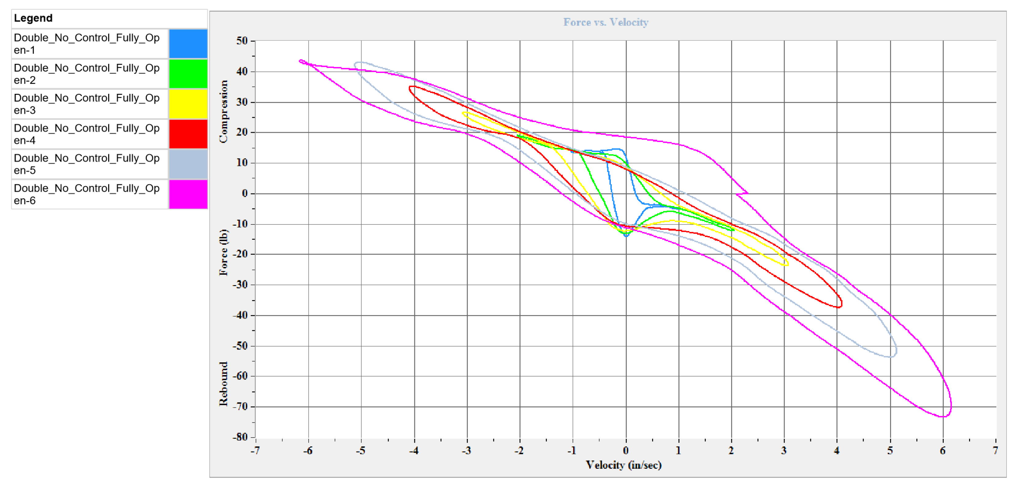
The passive double damper characteristics are obtained by performing the conventional Shock Dyno test routine of clamping the upper end of the Dyno and evaluating the Force variations of the damper to changes in the input displacements and velocities. Each of these graphs is plotted for different velocities ranging from 0.025–0.15 m/s (1–6 in/s), as shown in the legend of each plot, respectively. The contours in blue represent the operating condition of the damper at the lowest velocity i.e., 1 in/s (0.1 m/s). The velocities increase up to 6 in/s (0.15 m/s), in-unit increments, with the highest velocity shown by the pink contour.

Figure 8 shows the Force vs. Displacement plot of the double damper when it is subjected to no control algorithm, and the upper end of the Shock Dyno is not free to move. This condition resembles a passive damper as modeled by [18]. In this case, a continuous signal of +5 V is supplied to the solenoid valve which ensures that the valve is fully open during the entire test and the damping characteristics of the damper is at its minimum value. Each closed contour indicates the force-displacement plot at a specific velocity of the damper. The area under each contour shows the amount of energy absorbed by the damper for that cycle. The results agree with the literature that; as the velocity increases, the area under the contour plot increases.

Figure 9 shows the Force vs. Velocity plot of the damper when the solenoid valve is fully open. Similar to Figure 8, each contour indicates the force at a specific velocity of the damper. The hysteresis loop is observed during each cycle, indicating the presence of friction between the piston and the inner walls of the damper during the compression and the rebound stroke.

In order to observe the frequency domain characteristics and compare the dampers better, a method described in [27] is followed. In these experiments, the accelerometer data of the sprung mass and unsprung mass accelerations are recorded. The dampers are excited with a constant velocity in order to compare the response of the dampers to control logic.

The process followed for comparison of semi-active single damper and double damper performance can be seen in Figure 10. The single damper is initially tested for an unsprung input velocity of 0.2 m/sec, with a sampling frequency of 240 Hz. Fast Fourier transform of the signal is calculated by using Welch’s method to see the frequency domain characteristics and differentiate between the control algorithms better. Since the conversion of a signal from time domain to frequency domain is sensitive to effects of noise, it is necessary to have a method that would not be affected by the presence of stochastic noise in the signal. Instead of extracting the Fourier coefficients of the time domain signal, Welch’s method involving averaging and Hamming windowing Equation (2) is used.

$$\begin{array}{c}\hfill w\left(n\right)=0.54-0.46cos\left(2\pi \frac{n}{N}\right)\end{array}$$

(2)

where,

$0\le n\le N$

Window length L = N + 1

N is the total number of points

w are the coefficients of the Hamming window

The given signal is split into several sections using windowing techniques, and overlap. There is an overlap present between two consecutive sections in the signal. The power spectrum of each section, or window is computed, and overlapped hence eliminating effect of stochastic noise.

With this, the frequency domain plots for single semi-active damper with Skyhook control, single semi-active damper with Groundhook control, and double-semi active damper with Skyhook–Groundhook control are obtained. Two distinct zones of frequencies can be observed from Figure 11, around 1 Hz and 10 Hz. These are the chassis/sprung mass frequency and tire-hop frequencies, respectively. The areas under the Power Spectral Density (PSD) plot of the signal in the frequency domain in both low-frequency (chassis responses) and high frequencies (tire-hop) are a measure of the damping characteristic of a damper, as in Equation (3).

$$\begin{array}{c}\hfill G(X,f_1,f_2)={\int }_{f_1}^{f_2}{\left|X\left(f\right)\right|}^{2}df\end{array}$$

(3)

where, $G(X,f_1,f_2)$ represents a function that calculates the squared area under signal $X\left(f\right)$, in the range of frequencies of interest $f_1$ and $f_2$.

However, since the system is a discrete time system, numerical integration by trapezoidal method is used as in Equation (4).

$$\begin{array}{c}\hfill G(X,f_1,f_2)=\frac{f_2-f_1}{2N}\sum _{n=1}^N{(X\left(f_n\right)+X\left(f_{n+1}\right))}^2\end{array}$$

(4)

where, N are the number of points in the signal. This normalized cost function Equation (5) represents the “Comfort Cost,” which is used as a metric for evaluating the control algorithm.

$$\begin{array}{c}\hfill J_{comfort}=\frac{G(F_z,0,20)}{G(F^{no{m}_z},0,20)}\end{array}$$

(5)

where, $G(F_z^{nom},0,20)$ is the nominal (passive) reference suspension variance gains from 0 to 20 Hz; $G(F_z,0,20)$ is the variance gain of the system considered.

As seen in Figure 11, the area under the PSD plot in the chassis frequency zone is less for double damper with control, which signifies that the resonant peaks in that zone are damped, and the ride will be softer. In a nutshell, smaller the “Comfort cost,” the smoother is ride quality. Following this, the “Comfort cost” is evaluated by using the method shown in Figure 12. This “Comfort cost” is the power spectrum density around the chassis frequency zone (Figure 13) and the tire-hop frequency zone (Figure 14).

5. Results

It can be concluded from these “Comfort costs,” that the double-damper with Groundhook- Skyhook controller has a smaller cost value. Hence is giving a much smoother and softer ride as compared to the traditional Skyhook control and Groundhook control of the single-semi active damper. In addition to this, it is seen that in the tire-hop frequency zone, the double damper with control performs slightly worse than the single damper with control. This shows that the double damper with control is better suited for a softer ride, rather than for road holding. However, the performance of double damper with control in the tire-hop frequency zone can be better evaluated by using a dedicated quarter car test rig.

6. Conclusions

This paper deals with the implementation of a Hybrid Skyhook Groundhook control methodology on a novel double damper suspension system and its comparison with a conventional semi-active damper. The damper is equipped with multiple single axis accelerometers for measuring the accelerations of the unsprung mass, sprung mass and the body of the double damper. These measured accelerations are then used as inputs to the control algorithms. The semi-active control is implemented in real-time by varying the orifice diameter of the bypass valve as per the relative velocities of the different parts of the damper. The results have shown that the “comfort cost” associated with the semi-active double-damper has a smaller value as compared to the conventional semi-active single damper. This performance metric gives an indication that the double damper provides a smoother and a softer ride for the same input parameters as that of a semi-active single damper.

Future work will be focused on scaling down the double damper so it can be implemented on an actual vehicle. This provision will help evaluate the damper under different operating conditions such as road surfaces, velocity, and normal loads.