Random Nyström Approach to Clutter Subspace Estimation for Polarimetric Space-Time Adaptive Processing

Abstract

A random Nyström (R-Nyström) scheme for clutter subspace estimation is proposed in the context of polarimetric space-time adaptive processing (pSTAP). Unlike the standard Nyström scheme making use of only partial columns of the clutter plus noise covariance matrix (CNCM), R-Nyström exploits full CNCM information with a properly designed selection procedure under the newly developed random ridge cross leverage score (RRCLS) criterion. With R-Nyström, sup-ported by the complete CNCM columns, upgraded clutter subspace estimation can be achieved at the expense of an insignificant increase in computational complexity, in contrast to the standard Nyström. The R-Nyström-based pSTAP, termed pR-Nyström, is shown to be superior over the current eigendecomposition-free subspace pSTAP in the signal to clutter plus noise loss and computational complexity. The efficacy of R-Nyström/pR-Nyström is validated by the simulation results.

1. Introduction

Polarimetric space-time adaptive processing (pSTAP) plays an important role in improving the detection performance of airborne array radar operating in clutter environments [1,2,3,4]. The purpose of pSTAP is to suppress clutter by maximizing the signal to clutter plus noise ratio (SCNR) [5] in the cell under test (CUT), with the direct use of the clutter plus noise covariance matrix (CNCM). In pSTAP, the estimation accuracy of CNCM determines the performance of the processor. In general, CNCM can be estimated by using the independent and identically distributed (i.i.d.) training samples obtained from the adjacent range bins of CUT. However, in a real nonhomogeneous environment, the clutter characteristic in different range cells would change quickly and dynamically, which caused difficulty in collecting enough training samples [6].

Subspace-based methods have also been studied in the literature by using the principal subspace of CNCM instead. For example, the eigen-canceller method based on the direct eigenvalue decomposition (EVD) of CNCM was developed in [7]. This method, however, is not attractive for real-time processing due to its high computational complexity. For this reason, some fast subspace methods without EVD of CNCM have been proposed further. For instance, the projection approximation subspace tracking (PAST) scheme in [8] and the fast approximated power iteration (FAPI) scheme in [9]. Both schemes are implemented iteratively for the principal subspace estimation with some training samples available. A variant of PAST, called L1-PAST, was developed in [10], and incorporates an additional sparse constraint on the filter. These mentioned EVD-free subspace methods are computationally more efficient than the EVD method but suffer a severe performance loss in the estimation of the principal subspace.

The Nyström scheme is a popular technique for the fast estimation of the matrix representation of the principal subspace [11,12,13,14] while it was originally designed for solving the integral equations [15]. The main idea of Nyström is to select a subset called landmark points for the calculation of the kernel eigenfunction approximately. The most favored sampling method for subset selection is random sampling, which leads to the fast versions of kernel machines [16] and spectral clustering [17].

Although the random sampling method can work in practice, it will fail for many natural kernel matrices where the relative “importance” of points is not uniform across the dataset. A ridge leverage score (RLS) method is proposed for measuring the importance of points [18,19,20,21] such that the kernel matrices can be selected more reasonably. When the number of selected columns is fixed, the corresponding number of rows of the selection matrix is also fixed. The performance of the existing Nyström-based subspace estimation method is proportional to the number of selected columns. Therefore, it is worth studying improving the estimation accuracy of the principal subspace without increasing the selection number [22].

Most current Nyström variants employ only partial column information of CNCM. There is still room to improve the application of Nyström for estimating the clutter subspace. In this paper, we propose a new method called random Nyström (R-Nyström) which makes full use of CNCM under the newly developed “random” ridge cross leverage score (RRCLS) rule. In the RRCLS rule, a new selection matrix is constructed for obtaining the low-dimensional matrix in Nyström. The R-Nyström scheme can be directly applied for implementing high computational efficient pSTAP.

The major contributions of the paper are the following:

(1)

Enabling fast principal subspace identification within the Nyström framework while making full use of the CNCM information.

(2)

The computational burden in pSTAP can be reduced with high clutter suppression performance compared with the existing methods.

2. Data Model

Consider a side-looking uniform linear polarimetric radar array system with $N$ elements, each of which contains two independent polarimetric receiving channels. The inner-element spacing of the radar array $d$ is half of the radar wavelength. The geometry of the system is shown in Figure 1, where $(\theta ,\varphi )$ is the beam direction, and $v$ is the platform velocity. The polarimetric radar transmits uniformly $M$ pulses. The pulse repetition frequency (PRF) in a coherent processing interval (CPI) is $\iota$.

The radar data vector under the target free hypothesis ${\mathrm{H}}_0$ and the target presence hypothesis ${\mathrm{H}}_1$ can be written by

$$\{\begin{array}{c}{\mathrm{H}}_0:x=u\\ {\mathrm{H}}_1:x=t+u\end{array}$$

(1)

where $u=c+n$ is the clutter plus noise vector which is, as usual, a random vector drawn from a complex Gaussian process with zero-mean and unknown positive definite covariance matrix $R$; $t=Ap$ is the target polarization-space-time steering vector (or the target vector), $p$ is a complex random vector characterizing the unknown amplitude, phase, and polarization parameters of target return, and $A=I_2\otimes d_{f_{\mathbb{D}}}\otimes s_{f_{\mathbb{S}}}$, $f_{\mathbb{D}}=2v\cos \theta \cos \phi /(\lambda \iota )$ and $f_{\mathbb{S}}=d\cos \theta \cos \phi /\lambda$ denote the target normalized Doppler frequency and normalized spatial frequency, respectively; where $\otimes$ denotes the Kronecker product, $I_m$ denotes the $m\times m$ identity matrix, $\lambda$ is the radar wavelength, and

$$d_{f_{\mathbb{D}}}=M^{-1/2}{[1,{\mathrm{e}}^{ı2\mathsf{\pi }{f}_{\mathbb{D}}},\dots ,{\mathrm{e}}^{ı2\mathsf{\pi }(M-1)f_{\mathbb{D}}}]}^{\mathrm{T}}$$

(2)

$$s_{f_{\mathbb{S}}}=N^{-1/2}{[1,{\mathrm{e}}^{ı2\mathsf{\pi }{f}_{\mathbb{S}}},\dots ,{\mathrm{e}}^{ı2\mathsf{\pi }(N-1)f_{\mathbb{S}}}]}^{\mathrm{T}}$$

(3)

with $ı=\sqrt{-1}$, where superscript “$\mathrm{T}$” denotes transpose.

Following Ward’s clutter model [5] and polarization characterize [1], the $2MN\times 1$ vector $c$ can be written as follows

$$c=\left[\begin{array}{c}{c}_{\mathrm{H}}\\ c_{\mathrm{V}}\end{array}\right]={\displaystyle \sum _{n=1}^{N_{ℂ}}\underset{p_n}{\underbrace{\left[\begin{array}{c}{p}_{\mathrm{H},n}\\ p_{\mathrm{V},n}\end{array}\right]}}\otimes d_{f_{\mathbb{D},n}}\otimes s_{f_{\mathbb{S},n}}}$$

(4)

where $N_{ℂ}$ is the number of the independent clutter patches in one range cell, the $MN\times 1$ zero-mean complex Gaussian random vectors $c_{\mathrm{H}}$ and $c_{\mathrm{V}}$, given by

$$c_{\mathrm{H}}={\displaystyle \sum _{n=1}^{N_{ℂ}}{p}_{\mathrm{H},n}(d_{f_{\mathbb{D},n}}\otimes s_{f_{\mathbb{S},n}})}$$

(5)

$$c_{\mathrm{V}}={\displaystyle \sum _{n=1}^{N_{ℂ}}{p}_{\mathrm{V},n}(d_{f_{\mathbb{D},n}}\otimes s_{f_{\mathbb{S},n}})}$$

(6)

represent the horizontal and vertical clutter components whose covariance matrices are

$$R_{\mathrm{HH}}=E\{c_{\mathrm{H}}{c}_{\mathrm{H}}^{\mathrm{H}}\}={\displaystyle \sum _{n=1}^{N_{ℂ}}\underset{{\sigma }_{\mathrm{H},n}^2}{\underbrace{E\left\{\right|p_{\mathrm{H},n}{|}^2\}}}(d_{f_{\mathbb{D},n}}{d}_{f_{\mathbb{D},n}}^{\mathrm{H}})\otimes (s_{f_{\mathbb{S},n}}{s}_{f_{\mathbb{S},n}}^{\mathrm{H}})}$$

(7)

$$R_{\mathrm{VV}}=E\{c_{\mathrm{V}}{c}_{\mathrm{V}}^{\mathrm{H}}\}={\displaystyle \sum _{n=1}^{N_{ℂ}}\underset{{\sigma }_{\mathrm{V},n}^2}{\underbrace{E\left\{\right|p_{\mathrm{V},n}{|}^2\}}}(d_{f_{\mathbb{D},n}}{d}_{f_{\mathbb{D},n}}^{\mathrm{H}})\otimes (s_{f_{\mathbb{S},n}}{s}_{f_{\mathbb{S},n}}^{\mathrm{H}})}$$

(8)

in which $E\{\cdot \}$ denotes expectation and superscript “$\mathrm{H}$” denotes conjugate transpose; $f_{\mathbb{D},n}$ and $f_{\mathbb{S},n}$ are, respectively, the Doppler frequency and the spatial frequency of the nth clutter patch,

$$d_{f_{\mathbb{D},n}}=M^{-1/2}{[1,{\mathrm{e}}^{ı2\mathsf{\pi }{f}_{\mathbb{D},n}},\dots ,{\mathrm{e}}^{ı2\mathsf{\pi }(M-1)f_{\mathbb{D},n}}]}^{\mathrm{T}}$$

(9)

$$s_{f_{\mathbb{S},n}}=N^{-1/2}{[1,{\mathrm{e}}^{ı2\mathsf{\pi }{f}_{\mathbb{S},n}},\dots ,{\mathrm{e}}^{ı2\mathsf{\pi }(N-1)f_{\mathbb{S},n}}]}^{\mathrm{T}}$$

(10)

The $2\times 1$ vector $p_n$ can be written as $p_n=P^{1/2}{\mathsf{\rho }}_n$, where $E\left\{{\mathsf{\rho }}_n{\mathsf{\rho }}_n^{\mathrm{H}}\right\}={\sigma }_{\mathrm{H},n}^2{I}_2$, and

$$P=\left[\begin{array}{cc}1& \sqrt{\gamma }\zeta \\ \sqrt{\gamma }{\zeta }^{\ast }& \gamma \end{array}\right]$$

(11)

in which $\zeta$ and $\gamma$ are the correlation coefficient and the power ratio between the two polarimetric channels.

3. Clutter Subspace Based pSTAP

The clutter covariance matrix is

$$\begin{array}{cc}\hfill R_{\mathrm{c}}& =E\{c{c}^{\mathrm{H}}\}={\displaystyle \sum _{n=1}^{N_{ℂ}}E\{p_n{p}_n^{\mathrm{H}}\}\otimes d_{f_{\mathbb{D},n}}{d}_{f_{\mathbb{D},n}}^{\mathrm{H}}\otimes s_{f_{\mathbb{S},n}}{s}_{f_{\mathbb{S},n}}^{\mathrm{H}}}\hfill \\ & =P\otimes \left\{{\displaystyle \sum _{n=1}^{N_{ℂ}}{\sigma }_{\mathrm{H},n}^2(d_{f_{\mathbb{D},n}}{d}_{f_{\mathbb{D},n}}^{\mathrm{H}})\otimes (s_{f_{\mathbb{S},n}}{s}_{f_{\mathbb{S},n}}^{\mathrm{H}})}\right\}=P\otimes R_{\mathrm{HH}}\hfill \end{array}$$

(12)

According to [23], the effective rank of $R_{\mathrm{HH}}$ is $\lfloor N+\beta (M-1)\rfloor$, where $\lfloor .\rfloor$ denotes rounding to the nearest integer and $\beta =f_{\mathbb{D}}/f_{\mathbb{S}}=2v/(d\iota )$ denotes the slope of the clutter ridge. From (12), the effective rank of $R_{\mathrm{c}}$ is

$$\mathrm{rank}(R_{\mathrm{c}})=\mathrm{rank}(P)\times \mathrm{rank}(R_{\mathrm{HH}})$$

(13)

Because the rank of $P$ is 2, the effective rank of the clutter covariance matrix is

$$Q=\mathrm{rank}(R_{\mathrm{c}})=2\times \lfloor N+\beta (M-1)\rfloor$$

(14)

As the clutter and noise are independent, we have

$$R=R_{\mathrm{c}}+R_{\mathrm{n}}={\displaystyle \sum _{i=1}^{2MN}{\gamma }_i{v}_i{v}_i^{\mathrm{H}}}=U_{\mathrm{c}}{\Lambda }_{\mathrm{c}}{U}_{\mathrm{c}}^{\mathrm{H}}+{\sigma }^2{I}_{2MN}$$

(15)

Let $U_{\mathrm{c}}=[v_1,\cdots ,v_Q]$ whose column span is the so-called clutter subspace, ${\Lambda }_{\mathrm{c}}=\mathrm{diag}({\gamma }_1,\cdots ,{\gamma }_Q)$, which consists of the $Q$ principal eigenvalues of $R$, in which $\mathrm{diag}(\cdot )$ denotes a diagonal matrix; and ${\sigma }^2$ is the variance of the Gaussian white noise.

The optimal pSTAP filter vector is given by [3],

$$w_{\mathrm{opt}}=R^{-1}t=R^{-1}Ap$$

(16)

Applying the matrix inversion lemma to (15) yields

$$R^{-1}={(U_{\mathrm{c}}{\Lambda }_{\mathrm{c}}{U}_{\mathrm{c}}^{\mathrm{H}}+{\sigma }^2{I}_{2MN})}^{-1}={\sigma }^{-2}[I_{2MN}-U_{\mathrm{c}}{({\Lambda }_{\mathrm{c}}+{\sigma }^2{I}_{2MN})}^{-1}{\Lambda }_{\mathrm{c}}{U}_{\mathrm{c}}^{\mathrm{H}}]$$

(17)

Since the diagonal elements in $\Sigma$ are much larger than ${\sigma }^2$, (17) can be approximated as

$$R^{-1}\approx {\sigma }^{-2}(I_{2MN}-U_{\mathrm{c}}{U}_{\mathrm{c}}^{\mathrm{H}})$$

(18)

Therefore, the pSTAP filter vector can be written by

$$w=(I_{2MN}-U_{\mathrm{c}}{U}_{\mathrm{c}}^{\mathrm{H}})Ap$$

(19)

In the following, we give a new method for estimating $U_{\mathrm{c}}$ and $p$.

4. The Random Nyström Method

4.1. Revisit of Standard Nyström

The CNCM $R$ can be approximated as follows

$$R\approx \underset{U}{\underbrace{\left[\begin{array}{c}{U}_{11}\\ U_{21}\end{array}\right]}}\Lambda {\left[\begin{array}{c}{U}_{11}\\ U_{21}\end{array}\right]}^{\mathrm{H}}=\widehat{R}=\left[\begin{array}{cc}\underset{{\widehat{R}}_{11}}{\underbrace{U_{11}\Lambda U_{11}^{\mathrm{H}}}}& \underset{{\widehat{R}}_{21}^{\mathrm{H}}}{\underbrace{U_{11}\Lambda U_{21}^{\mathrm{H}}}}\\ \underset{{\widehat{R}}_{21}}{\underbrace{U_{21}\Lambda U_{11}^{\mathrm{H}}}}& \underset{{\widehat{R}}_{22}={\widehat{R}}_{21}{\widehat{R}}_{11}^{-1}{\widehat{R}}_{21}^{\mathrm{H}}}{\underbrace{U_{21}\Lambda U_{21}^{\mathrm{H}}}}\end{array}\right]$$

(20)

where $U$ is an $2MN\times Q$ orthogonal matrix whose columns are the $Q$ principal eigenvectors of $R$, $\Lambda$ is a diagonal matrix whose diagonal elements are the $Q$ principal eigenvalues of $R$; $U_{11}\in {ℂ}^{K\times Q}$, and $U_{21}\in {ℂ}^{(2MN-K)\times Q}$, with $Q\le K<2MN$.

Let

$$\widehat{C}=\widehat{R}\underset{S}{\underbrace{\left[\begin{array}{c}{S}_{11}\\ S_{21}\end{array}\right]}}=\left[\begin{array}{c}{\widehat{C}}_{11}\\ {\widehat{C}}_{21}\end{array}\right]=\left[\begin{array}{c}{\widehat{R}}_{11}{S}_{11}+{\widehat{R}}_{21}^{\mathrm{H}}{S}_{21}\\ {\widehat{R}}_{21}{S}_{11}+{\widehat{R}}_{21}{\widehat{R}}_{11}^{-1}{\widehat{R}}_{21}^{\mathrm{H}}{S}_{21}\end{array}\right]$$

(21)

where $S$ is a $2MN\times K$ selection matrix, and $S_{11}\in {ℂ}^{K\times K}$, and $S_{21}\in {ℂ}^{(2MN-K)\times K}$. In the standard Nyström, $S$ is composed of $K$ different but arbitrary columns of $I_{2MN}$.

Define then

$$\widehat{U}=\left[\begin{array}{c}{\widehat{U}}_{11}\\ {\widehat{U}}_{21}\end{array}\right]$$

(22)

where ${\widehat{U}}_{21}={\widehat{C}}_{21}{\widehat{U}}_{11}{\widehat{\Lambda }}_{11}^{-1}$, in which ${\widehat{U}}_{11}$ is an $K\times Q$ orthogonal matrix whose columns are the eigenvectors of ${\widehat{C}}_{11}$, and ${\widehat{\Lambda }}_{11}$ is the $Q\times Q$ diagonal matrix whose diagonal elements are the eigenvalues of ${\widehat{C}}_{11}$.

It can be verified that $\mathrm{rank}(\widehat{U})=Q$, and

$$\widehat{U}{\widehat{\Lambda }}_{11}=\left[\begin{array}{c}{\widehat{U}}_{11}{\widehat{\Lambda }}_{11}\\ {\widehat{U}}_{21}{\widehat{\Lambda }}_{11}\end{array}\right]=\left[\begin{array}{c}{\widehat{C}}_{11}\\ {\widehat{C}}_{21}\end{array}\right]{\widehat{U}}_{11}=U\Lambda U^{\mathrm{H}}S{\widehat{U}}_{11}$$

(23)

It follows that

$$\widehat{U}=U(\Lambda U^{\mathrm{H}}S{\widehat{U}}_{11}{\widehat{\Lambda }}_{11}^{-1})$$

(24)

This implies that $\mathrm{span}(\widehat{U})=\mathrm{span}(U)$, which is exactly the Q-dimensional clutter subspace to be identified.

The computational complexity of the standard Nyström is about $O(2MN{K}^2)$. If $K<<2MN$, it is computationally much simpler than the classical eigendecomposition method whose computational complexity is about $O({(2MN)}^3)$. However, making use of a relatively small $K$ in the method would result in poor identification $\mathrm{span}(U)$ since only $K$ columns of $R$ are employed. In the sequel, a R-Nyström method is developed which fulfills a good compromise between the computational complexity and identification performance. In the new method, the dimension of the selection matrix $S$ is still of $2MN\times K$. However, each column of $S$ is designed by a new criterion based on $R$. Note that all Nyström-based methods require EVD operation, except that R-Nyström is based on a low-dimensional matrix for EVD.

4.2. The Random Nyström Method

To show the estimated performance of the clutter subspace from $R$, a cost function (projection error) which denotes the difference between the estimated and the real projection operator of the clutter subspace is given. The smaller the function, the more accurate the estimation. The cost function is given by

$$f(U_{\mathrm{e}})=\underset{U_{\mathrm{e}}}{\min }\left|\right|U_{\mathrm{e}}{(U_{\mathrm{e}}^{\mathrm{H}}{U}_{\mathrm{e}})}^{-1}{U}_{\mathrm{e}}^{\mathrm{H}}-U_{\mathrm{r}}{U}_{\mathrm{r}}^{\mathrm{H}}|{|}_{\mathrm{F}}$$

(25)

where $U_{\mathrm{e}}$ and $U_{\mathrm{r}}$ denote the estimated and real matrix representation of the clutter subspace, respectively; $\left|\right|\cdot |{|}_{\mathrm{F}}$ denotes the Frobenius norm. Because the estimated matrix $U_{\mathrm{e}}$ is not a column orthogonal matrix, the projection operator is used by $U_{\mathrm{e}}{(U_{\mathrm{e}}^{\mathrm{H}}{U}_{\mathrm{e}})}^{-1}{U}_{\mathrm{e}}^{\mathrm{H}}$ in (25). Observed from the standard Nyström method in part 4.1, $U_{\mathrm{e}}$ is determined by the selection matrix $S$. Therefore, $f(U_{\mathrm{e}})$ is also determined by $S$. In the following, a new criterion is proposed to determine the selection matrix $S$.

Define a $2MN\times K$ matrix $S$, and assume all the elements in $S$ are determined with $B(i,j)$ as the probability distribution function, namely the value at $(i,j)$ depends on $B(i,j)$. Let $S(i,j)$ be the function at $(i,j)$ of matrix $S$ whose definition is represented as follows [24]

$$S(i,j)=\{\begin{array}{c}1,E(i,j)\le B(i,j)\\ 0,E(i,j)>B(i,j)\end{array}$$

(26)

where $E(i,j)$ is a uniformly distributed random number between [0,1].

The derivation of $B(i,j)$ is given in the following. First, perform singular value decomposition (SVD) for $R$,

$$R=U^{\prime }{\Sigma }^{\prime }{V^{\prime }}^{\mathrm{H}}$$

(27)

where $U^{\prime }=[{u^{\prime }}_1,{u^{\prime }}_2,\cdots ,{u^{\prime }}_{2MN}]$, $V^{\prime }=[{v^{\prime }}_1,{v^{\prime }}_2,\cdots ,{v^{\prime }}_{2MN}]$, and ${\Sigma }^{\prime }=\mathrm{diag}\{{{\sigma }^{\prime }}_1,{{\sigma }^{\prime }}_2,\cdots ,{{\sigma }^{\prime }}_{2MN}\}$ with ${{\sigma }^{\prime }}_1\ge {{\sigma }^{\prime }}_2\ge \cdots \ge {{\sigma }^{\prime }}_{2MN}\ge 0$.

The jth column of $R$ can be represented as follows

$$R_j={\displaystyle \sum _{q=1}^Q{{\sigma }^{\prime }}_q{u^{\prime }}_q{({v^{\prime }}_{q,j})}^{\ast }}={\displaystyle \sum _{q=1}^Q[{{\sigma }^{\prime }}_q{({v^{\prime }}_{q,j})}^{\ast }]{u^{\prime }}_q}$$

(28)

where ${v^{\prime }}_{q,j}$ is the jth element of the qth right singular vector, and “$\ast$” denotes a conjugate. Observed from (28), $R_j$ is a linear combination of the left singular vectors and right singular values, and the coefficients are the corresponding jth row of $V^{\prime }$. Hence, $R_j$ can be approximated with a linear combination of the larger $K$ left singular vectors and its corresponding singular values

$$R_j\approx {\displaystyle \sum _{q=1}^K[{{\sigma }^{\prime }}_q{({v^{\prime }}_{q,j})}^{\ast }]{u^{\prime }}_q}$$

(29)

All the coefficients are extracted and used to construct the normalized statistical leverage score, which is represented as follows

$${\epsilon }_j=\frac{1}{K}{\displaystyle \sum _{k=1}^K{[{({v^{\prime }}_{q,j})}^{\ast }]}^2}$$

(30)

where ${\epsilon }_j>0$, ${\displaystyle {\sum }_{j=1}^{2MN}{\epsilon }_j}=1$ and $1\le j\le 2MN$. The whole leverage scores form a probability distribution over the $2MN$ columns [18]. A new RRCLS based on related works on RLS [19,20,21,22] can be defined by

$${\tau }_{i,j}={\{{[DR{(R+\kappa I)}^{-1}]}^{\mathrm{T}}\}}_{i,j}$$

(31)

in which $D$ is a $K\times 2MN$ matrix whose elements follow a standard normal distribution, $\kappa$ is a constant and $1\le i\le 2MN$, $1\le j\le K$. $B(i,j)$ can be obtained by

$$B(i,j)=\min \{1,\delta {\tau }_{i,j}\}$$

(32)

where $\delta$ is an adjustable factor. After obtaining the probability distribution function $B(i,j)$, the selection matrix $S$ can be determined by (26). Compared to the standard Nyström, the number of non-zero elements in each column of $S$ is more than one.

The selected low dimension matrix can be represented as

$$\tilde{R}=RS=\left[\begin{array}{c}{\tilde{R}}_{11}\\ {\tilde{R}}_{21}\end{array}\right]$$

(33)

Similar to (22), define

$$\tilde{U}=\left[\begin{array}{c}{\tilde{U}}_{11}\\ {\tilde{U}}_{21}\end{array}\right]$$

(34)

where ${\tilde{U}}_{21}={\tilde{R}}_{21}{\tilde{U}}_{11}{\tilde{\Lambda }}_{11}^{-1}$, in which ${\tilde{U}}_{11}$ is an $K\times Q$ orthonormal matrix whose columns are the eigenvectors of ${\tilde{R}}_{11}$, and ${\tilde{\Lambda }}_{11}$ is the $Q\times Q$ diagonal matrix whose diagonal elements are the eigenvalues of ${\tilde{R}}_{11}$. Note that all the columns of $\tilde{U}$ are not orthogonal to each other.

The R-Nyström algorithm for the matrix representation of the clutter subspace is summarized as follows:

(a)

determine the selection matrix $S$ by (26), (31) and (32)

(b)

obtain the low-dimensional matrix by (33)

(c)

estimate the matrix representation of the clutter subspace by (34)

4.3. Application of R-Nyström to pSTAP

The CNCM $R$ is given by the sample estimate

$$\overline{R}=E\{u{u}^{\mathrm{H}}\}\approx \frac{1}{L}{\displaystyle \sum _{l=1}^L{u}_l{u}_l^{\mathrm{H}}}$$

(35)

where $u_l$ is the clutter plus noise vector of the lth range cell and $L$ is the number of training samples.

Substitute (35) into (31), the new RRCLS can be written as

$${\overline{\tau }}_{i,j}={\{{[D\overline{R}{(\overline{R}+\kappa I)}^{-1}]}^{\mathrm{T}}\}}_{i,j}$$

(36)

By (36), the corresponding $\overline{B}(i,j)$ can be written as

$$\overline{B}(i,j)=\min \{1,\delta {\overline{\tau }}_{i,j}\}$$

(37)

Therefore, the new selection matrix $\overline{S}$ is calculated by

$$\overline{S}(i,j)=\{\begin{array}{c}1,E(i,j)\le \overline{B}(i,j)\\ 0,E(i,j)>\overline{B}(i,j)\end{array}$$

(38)

Because there is an error in the sample estimate, $x$ in ${\mathrm{H}}_0$ is processed directly for avoiding estimation error into the following calculation. The selected output is written by

$$y={\overline{S}}^{\mathrm{H}}x$$

(39)

and the corresponding low-dimensional matrices are given by

$$R_{yy}=E\{y{y}^{\mathrm{H}}\}\approx {\overline{S}}^{\mathrm{H}}\overline{R}\overline{S}$$

(40)

$$R_{xy}=E\{x{y}^{\mathrm{H}}\}=\overline{R}\overline{S}$$

(41)

Then, performing EVD of $R_{yy}$ yields,

$$R_{yy}={\displaystyle \sum _{i=1}^K{\lambda }_i{\overline{u}}_i{\overline{u}}_i^{\mathrm{H}}}$$

(42)

where ${\lambda }_i$ (${\lambda }_1\ge \cdots \ge {\lambda }_Q>{\lambda }_{Q+1}=\cdots ={\lambda }_K$) is the eigenvalue of $R_{yy}$ and ${\overline{u}}_i$ is the corresponding eigenvector. Let ${\overline{U}}_{yy}=[{\overline{u}}_1,{\overline{u}}_2,\cdots ,{\overline{u}}_Q]$ and ${\overline{\Lambda }}_{yy}=\mathrm{diag}({\lambda }_1,{\lambda }_2,\cdots ,{\lambda }_Q)$, and the matrix representation of the clutter subspace is given by

$$\overline{U}=R_{xy}{\overline{U}}_{yy}{\overline{\Lambda }}_{yy}^{-1}$$

(43)

The columns of $\overline{U}$ are also not mutually orthogonal. Based on (19), the weight vector of the pR-Nyström method is given by

$$w_{\mathrm{pR}-\mathrm{Nystrom}}=(I_{2MN}-\overline{U}{({\overline{U}}^{\mathrm{H}}\overline{U})}^{-1}{\overline{U}}^{\mathrm{H}})Ap$$

(44)

It notes that the polarimetric signal vector to be detected is unknown in advance, hence, $p$ needs to be estimated by the proposed modified least square method (mLSM). In hypothesis ${\mathrm{H}}_1$, the radar data are represented as follows

$$x=Ap+c+n$$

(45)

Introduce function $f(p)$, which is written by

$$f(p)=\left|\right|Ap-x^{\prime }|{|}_2^2$$

(46)

where $x^{\prime }=x-c$ denotes the data that contain no clutter components. For eliminating the clutter effect in $x$, $x^{\prime }$ can be obtained by projecting $x$ into the orthogonal subspace of clutter subspace, where the matrix representation of the clutter subspace $\widehat{U}$ can be obtained by the standard Nyström method,

$$x^{\prime }=[I_{2MN}-\widehat{U}{({\widehat{U}}^{\mathrm{H}}\widehat{U})}^{-1}{\widehat{U}}^{\mathrm{H}}]x$$

(47)

Substitute (47) into (46),

$$f(p)=||Ap-[I_{2MN}-\widehat{U}{({\widehat{U}}^{\mathrm{H}}\widehat{U})}^{-1}{\widehat{U}}^{\mathrm{H}}]x|{|}_2^2$$

(48)

Therefore, when $\widehat{p}=p$, $f(p)$ can get the minimum value. Let

$$\widehat{p}=\arg \min \{||Ap-[I_{2MN}-\widehat{U}{({\widehat{U}}^{\mathrm{H}}\widehat{U})}^{-1}{\widehat{U}}^{\mathrm{H}}]x|{|}_2^2\}$$

(49)

Taking the sub-gradient of (49) with respect to $p$, $\widehat{p}$ can be obtained as follows

$$\widehat{p}={(A^{\mathrm{H}}A)}^{-1}{A}^{\mathrm{H}}[I_{2MN}-\widehat{U}{({\widehat{U}}^{\mathrm{H}}\widehat{U})}^{-1}{\widehat{U}}^{\mathrm{H}}]x$$

(50)

The final filter vector is rewritten as

$${\widehat{w}}_{\mathrm{pR}-\mathrm{Nystrom}}=(I_{2MN}-\overline{U}{({\overline{U}}^{\mathrm{H}}\overline{U})}^{-1}{\overline{U}}^{\mathrm{H}})A{(A^{\mathrm{H}}A)}^{-1}{A}^{\mathrm{H}}[I_{2MN}-\widehat{U}{({\widehat{U}}^{\mathrm{H}}\widehat{U})}^{-1}{\widehat{U}}^{\mathrm{H}}]x$$

(51)

Extend the existing methods to the pSTAP case, which are called pEVD, pPAST, pFAPI, pL1-PAST, and pBiPerEFA, respectively. Note that all the methods use the estimated $\widehat{p}$ in the process of calculating the corresponding filter.

5. Computational Complexity Analysis

The major computational burden of the pR-Nyström method is engaged with the calculation for the selection matrix and the polarimetric signal vector to be detected. The main polarimetric radar system parameters are as shown in

Table 1. Polarimetric radar system parameters.

Parameter	Value
antenna array	side-looking array
the number of antennas	16
pulse number in one CPI	16
CNR	40 dB
PRF	1200
velocity	200 m/s
airborne height	9 km
looking direction	0°
target auxiliary polarization angle	30°
target polarization phase difference	60°
clutter degree of polarization	0.99
the power ratio between two channels	1
clutter statistical average phase difference	90°

, and are the same as that in [2]. The approximate computational complexity and the averaged computation time of 100 independent runs are listed in

Table 2. Complexity and computation time comparison.

Method	Complexity	Time/ms
mLSM	$t_1=O\left(\begin{array}{l}{K}^2(3K+2L-2)+MNK(4L+8MN+16K-8)\\ +4MN(4M^2{N}^2+MN+4)+16\end{array}\right)$	15.0
pEVD	$O\left(\begin{array}{l}8M^3{N}^3+16M^2{N}^{2}L+8M^2{N}^{2}K\\ +56M^2{N}^2-2MN(L-12)+4\end{array}\right)+t_1$	59.5
pPAST	$O\left(\begin{array}{l}60M^2{N}^2+(8MN+6K^2-3)KL\\ +8M^2{N}^2(K+L)-4MN(L-6)+4\end{array}\right)+t_1$	47.8
pFAPI	$O\left(\begin{array}{l}(8K^2+8K-7)K+8M^2{N}^2(2K+L)\\ +2MN(K-L+12)+60M^2{N}^2+4\end{array}\right)+t_1$	50.1
pL1-PAST	$O\left(\begin{array}{l}60M^2{N}^2+(6K^2+6MN+4MNK-2K-2)KL\\ -4MN(L-6)+8M^2{N}^2(K+L)\end{array}\right)+t_1$	126.9
pNyström	$O\left(\begin{array}{l}4K^3+(2K-1)(10MNK+8M^2{N}^2)\\ +(2L-1)(K^2+2MNK)+2MN(4MN-1)\end{array}\right)+t_1$	21.5
pR-Nyström	$O\left(\begin{array}{l}4K^3+K(2KL-K-L)+2MN(16KL-6K-L+12)\\ +4M^2{N}^2(2MN+2K+6L+14)+4\end{array}\right)+t_1$	36.4
pBiPerEFA	$O\left(\begin{array}{l}8MNL(MN+3)+2MN(22MN+84N+11)\\ -6N(6N+L)+54(108N^3+126N^2+26N-3)\end{array}\right)+t_1$	29.4

, where the number of training samples is $L=130$ and $K=Q$ under the following configurations: (1) CPU: Intel(R) Core (TM) i7-6700 3.40 GHz; (2) memory: 8.00 GB; (3) system: 64-bit Windows 7; (4) MATLAB R2016a.

It can be seen from Table 2 that the average computation time of the mLSM method is denoted as $t_1$, and the average computation time of the pR-Nyström method is less than that of the other existing methods except for the pNyström method and pBi-PerEFA method. The EFA referred to in this paper is with three Doppler bins and the iteration number of pBiPerEFA method [25] is nine.

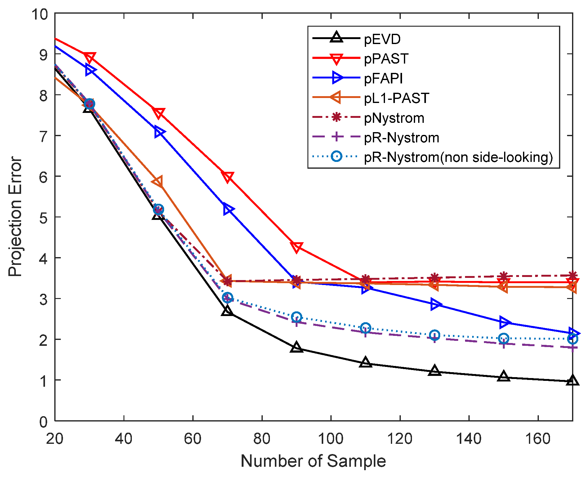
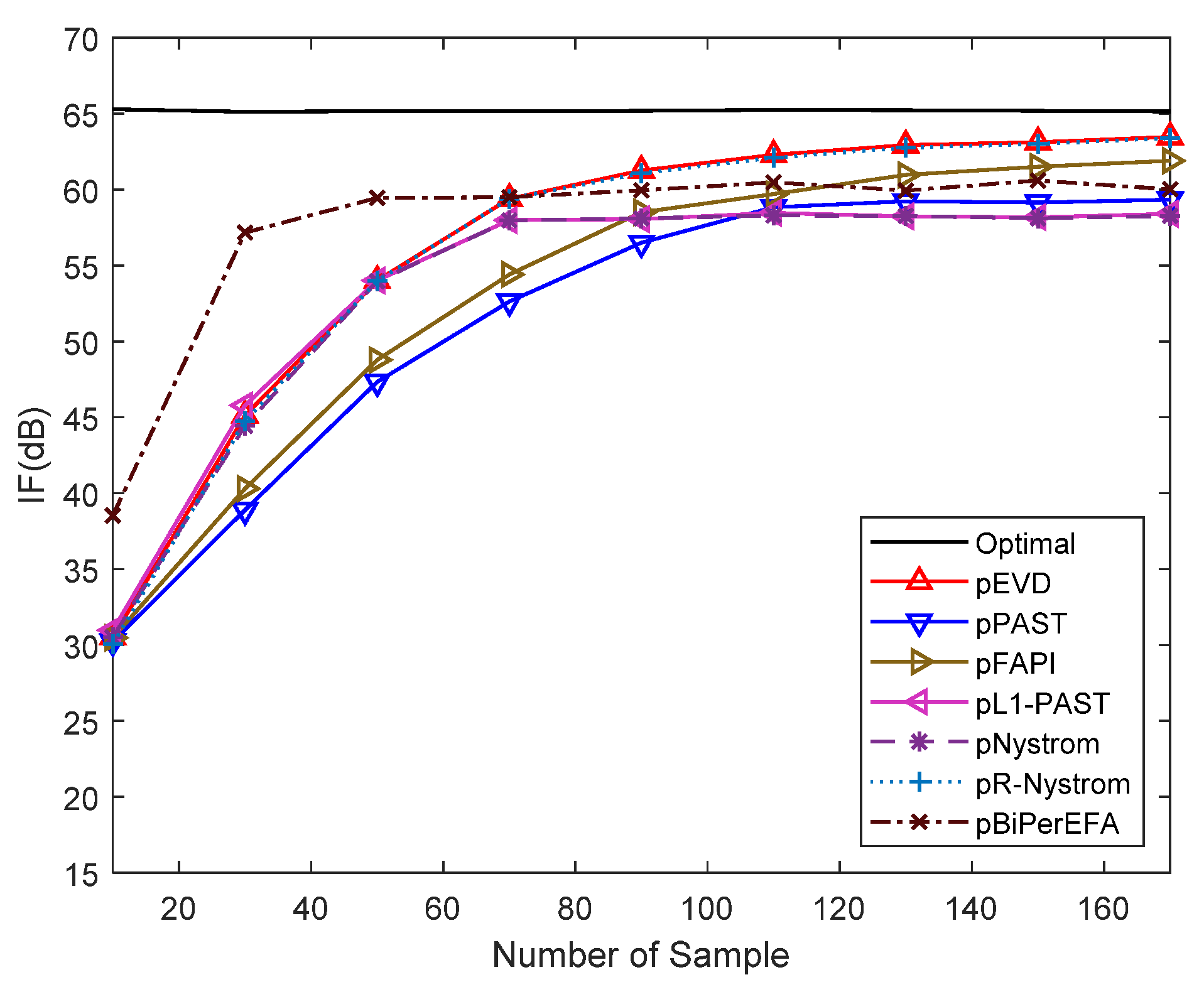
6. Numerical Results

In this section, to assess SCNR loss, simulated data are employed as the metric for comparison among different methods, which is defined by

$$\mathrm{SCNR}\mathrm{loss}=\frac{{\mathrm{SCNR}}_o}{{\mathrm{SCNR}}_i}=\frac{|{\widehat{w}}^{\mathrm{H}}\widehat{t}{|}^2}{({\widehat{w}}^{\mathrm{H}}{R}_{\mathrm{real}}\widehat{w})({\widehat{t}}^{\mathrm{H}}\widehat{t})}$$

(52)

where ${\mathrm{SCNR}}_o$ and ${\mathrm{SCNR}}_i$ denote the output and input signal to clutter plus noise ratio, respectively; $R_{\mathrm{real}}$ represents the true CNCM which is assumed to be known in simulation experiments and $\widehat{t}=A\widehat{p}$. The polarimetric radar system parameters are shown in Table 1, and $\kappa =1$. The curves shown are the averaged results of 100 Monte Carlo trials.

Shown in Figure 2 are the projection error curves versus training samples with different values of $\delta$, where the target normalized Doppler frequency is 0.2. It is observed that the pR-Nyström method is robust for different values of $\delta$ between $[10,40]$. In the following simulation, we set $\delta =20$.

Shown in Figure 3 are the projection error curves versus training samples, where the target normalized Doppler frequency is 0.2. It is observed that the pR-Nyström method has a smaller projection error and is closest to the pEVD method. This indicates that the pR-Nyström method has a better approximate performance than the other methods. Furthermore, in the case of the non-side-looking model, assuming that the angle between the array pointing and the direction of movement is 30°, the SCNR loss is a little weaker than the side-looking model.

Shown in Figure 4 are the SCNR loss curves versus training samples where the target normalized Doppler frequency is 0.2. It is observed that the pR-Nyström method has a better SCNR loss performance than the other methods with the increase in the training sample and is closest to the pEVD method.

Shown in Figure 5 are the SCNR loss curves versus the target normalized Doppler frequency, where the number of training samples is 130. It is observed that the pR-Nyström method can achieve a better SCNR loss performance than the other methods with different target normalized Doppler frequencies and is closest to the pEVD method.

Shown in Figure 6 are the SCNR loss curves versus the normalized Doppler frequency, with different clutter degree of polarization (DOP). The number of training samples is 130, and CNR = 40 dB. It is observed that when the target Doppler frequency is large, the SNCR loss performance of the pR-Nyström method stays stable with different DOPs; when the normalized Doppler frequency value is located in [−0.1, 0.1], the SCNR loss performance of pR-Nyström method changes. When the clutter DOP is large, the clutter is a completely polarized wave and this will make a larger notch [2]. When the clutter DOP is gradually reduced, the clutter presents a partially polarized wave and this leads to deeper and deeper notch.

Shown in Figure 7 are the SCNR loss curves versus the normalized Doppler frequency, with different CNRs. The number of training samples is 130, and $\left|\zeta \right|=0.99$. It is observed that the pR-Nyström method has a stable SCNR loss performance when the normalized Doppler frequency value is large. When the normalized Doppler frequency value is located in $[-0.1, 0.1]$, the SCNR loss performance of the pR-Nyström method changes with different CNRs. The reason is that when the clutter notch is formed in the main lobe clutter region of Doppler frequency by the clutter suppressor, its depth depends on the CNR. The clutter in the side lobe clutter region can be well suppressed to the noise level and is less affected by the CNR.

7. Conclusions

We have presented a random Nyström framework based on the matrix representation of the clutter subspace estimation method for pSTAP. The new method involves a new selection matrix for the complete use of CNCM, which is determined by the proposed random ridge cross leverage score rule. Simulation results show that the proposed method has an appealing clutter suppression performance and computational efficiency as compared with the existing methods.

It can be seen from the investigation in this article that high subspace estimation accuracy and computational efficiency can be achieved based on the new column selection criterion within the Nyström framework. In order to reduce the influence of adjustable factors on subspace estimation, the number of adjustable factors in the column selection criterion should be as small as possible. Hence, it is important to investigate further the adjustable factors in the subsequent research. When the newly proposed method is applied in airborne radar, the clutter suppression performance of pSTAP can be improved, and the target detection probability can be increased.

References

1. Park, H.R.; Wang, H.; Li, J. An adaptive polarization-space-time processor for radar system. In Proceedings of the IEEE Antennas and Propagation Society International Symposium, Ann Arbor, MI, USA, 28 June–2 July 1993; pp. 698–701. [Google Scholar]
2. Wu, D.; Xu, Z.; Zhang, L.; Xiong, Z.; Xiao, S. Performance analysis of polarization-space-time three-domain joint processing for clutter suppression in air-borne radar. Prog. Electromagn. Res. 2012, 129, 579–601. [Google Scholar] [CrossRef] [Green Version]
3. Wu, D.; Xu, Z.; Xiong, Z.; Zhang, L.; Xiao, S. Polarization-space-time joint domain processing for clutter suppression in subspace leakage environments. In Proceedings of the 2011 IEEE CIE International Conference on Radar, Chengdu, China, 24–27 October 2011; pp. 692–695. [Google Scholar]
4. Du, W.; Liao, G.; Yang, Z. Clutter space-time covariance matrix estimate based on multi-polarised data. IET Radar Sonar Navig. 2014, 8, 1109–1115. [Google Scholar] [CrossRef]
5. Ward, J. Space-Time Adaptive Processing for Airborne Radar; IET: London, UK, 1998. [Google Scholar]
6. Melvin, W.L. Space-time adaptive radar performance in heterogeneous clutter. IEEE Trans. Aerosp. Electron. Syst. 2000, 36, 621–633. [Google Scholar] [CrossRef]
7. Wang, Z.; Wang, Y.; Duan, K.; Xie, W. Subspace-augmented clutter suppression technique for STAP radar. IEEE Geosci. Remote Sens. Lett. 2016, 13, 462–466. [Google Scholar] [CrossRef]
8. Yang, B. Projection approximation subspace tracking. IEEE Trans. Signal Process. 1995, 43, 95–107. [Google Scholar] [CrossRef]
9. Badeau, R.; David, B.; Richard, G. Fast approximated power iteration subspace tracking. IEEE Trans. Signal Process. 2005, 53, 2931–2941. [Google Scholar] [CrossRef] [Green Version]
10. Yang, X.; Sun, Y.; Zeng, T.; Long, T.; Sarkar, T.K. Fast STAP method based on PAST with sparse constraint for airborne phased array radar. IEEE Trans. Signal Process. 2016, 64, 4550–4561. [Google Scholar] [CrossRef]
11. Zhang, K.; Kwok, J.T. Clustered Nyström method for large scale manifold learning and dimension reduction. IEEE Trans. Neural Netw. 2010, 21, 1576–1587. [Google Scholar] [CrossRef] [PubMed] [Green Version]
12. Kumar, S.; Mohri, M.; Talwalkar, A. Sampling methods for the Nyström method. J. Mach. Learn. Res. 2012, 13, 981–1006. [Google Scholar]
13. Wang, S.; Zhang, Z. Improving CUR matrix decomposition and the Nyström approximation via adaptive sampling. J. Mach. Learn. Res. 2013, 14, 2729–2769. [Google Scholar]
14. Qian, C.; Huang, L.; So, H.C. Computationally efficient ESPRIT algorithm for direction-of-arrival estimation based on Nyström method. Signal Process. 2014, 94, 74–80. [Google Scholar] [CrossRef]
15. Baker, C.T.H. The Numerical Treatment of Integral Equations; Oxford University Press: Oxford, UK, 1978. [Google Scholar]
16. Williams, C.K.I.; Seeger, M. Using the Nyström method to speed up kernel machines. In Proceedings of the 13th International Conference on Neural Information Processing Systems; MIT Press: Cambridge, MA, USA, 2000. [Google Scholar]
17. Fowlkes, C.; Belongie, S.; Chung, F.; Malik, J. Spectral grouping using the Nyström method. IEEE Trans. Pattern Anal. Mach. Intell. 2004, 26, 214–225. [Google Scholar] [CrossRef] [PubMed] [Green Version]
18. Drineas, P.; Magdon-Ismail, M.; Mahoney, M.W.; Woodruff, D.P. Fast approximation of matrix coherence and statistical leverage. J. Mach. Learn. Res. 2012, 13, 3475–3506. [Google Scholar]
19. Cohen, M.B.; Musco, C.; Musco, C. Ridge leverage scores for low-rank approximation. arXiv 2015, arXiv:1511.07263. [Google Scholar]
20. Calandriello, D.; Lazaric, A.; Valko, M. Analysis of Nyström method with sequential ridge leverage score sampling. In Proceedings of the 2016 Thirty-Second Conference on Uncertainty in Artificial Intelligence, New York, NY, USA, 25–29 June 2016. [Google Scholar]
21. Musco, C.; Musco, C. Recursive sampling for the Nyström method. In Proceedings of the 31st Conference on Neural Information Processing Systems (NIPS 2017), Long Beach, CA, USA, 4–9 December 2017. [Google Scholar]
22. Wang, W.; Chen, Z.; Li, X.; Wang, B. Space time adaptive processing algorithm for multiple-input-multiple-output radar based on Nyström method. IET Radar Sonar Navig. 2016, 10, 459–467. [Google Scholar] [CrossRef]
23. Reed, I.S.; Mallet, J.D.; Brennan, L.E. Rapid convergence rate in adaptive arrays. IEEE Trans. Aerosp. Electron. Syst. 1974, AES-10, 853–863. [Google Scholar] [CrossRef]
24. Smith, M.S.; Tan, T.G. Sidelobe reduction using random methods for antenna arrays. Electron. Lett. 1983, 19, 931–933. [Google Scholar] [CrossRef]
25. Zhou, Y.; Chen, X.; Li, Y.; Li, Y.; Wang, L.; Jiang, B.; Fang, D. A fast STAP method using persymmetry covariance matrix estimation for clutter suppression in airborne MIMO radar. EURASIP J. Adv. Signal Process. 2019, 2019, 13. [Google Scholar] [CrossRef]
Figure 1. The geometry of polarimetric radar array.
Electronics 09 01488 g001
Figure 2. Projection error versus training samples: with different δ .
Electronics 09 01488 g002
Figure 3. Projection error versus training samples.
Electronics 09 01488 g003
Figure 4. Signal to clutter plus noise ratio (SCNR) loss performance versus training samples.
Electronics 09 01488 g004
Figure 5. SCNR loss performance versus target Doppler frequency.
Electronics 09 01488 g005
Figure 6. SCNR loss performance versus target Doppler frequency: with different clutter degrees of polarization (DOPs).
Electronics 09 01488 g006
Figure 7. SCNR loss performance versus target Doppler frequency: with different clutter to noise ratio (CNR).
Electronics 09 01488 g007