Staging Melanocytic Skin Neoplasms Using High-Level Pixel-Based Features


Abstract
:1. Introduction
2. Related Work
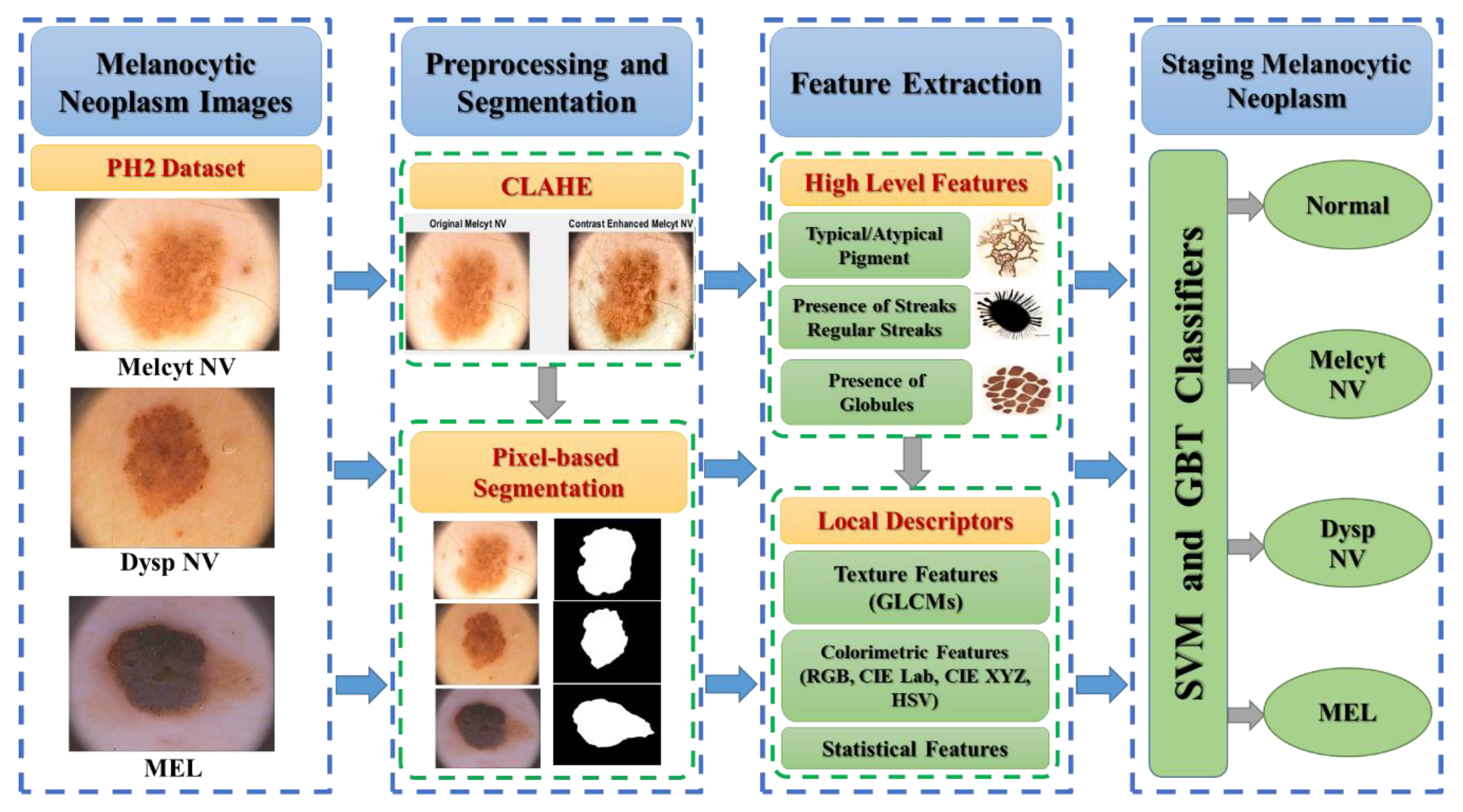
3. The Proposed Framework
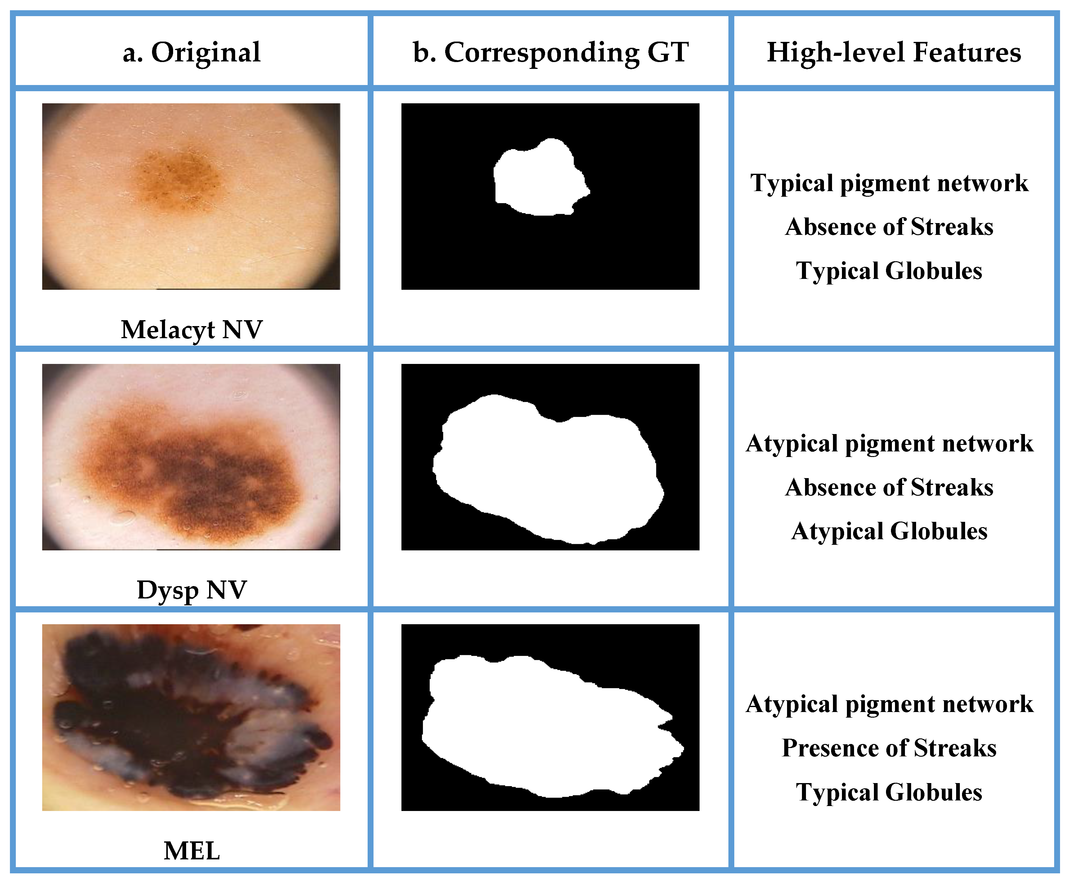
3.1. Pre-Processing and Segmentation
3.2. Feature Extraction
3.2.1. Morphological Boundary Shape Descriptor
Binary Dilation
Grayscale Dilation
Binary Erosion
Grayscale Erosion
3.2.2. Local Feature Descriptors
3.3. Feature Reduction
3.4. Classification of Melanocytic Dermoscopic Images
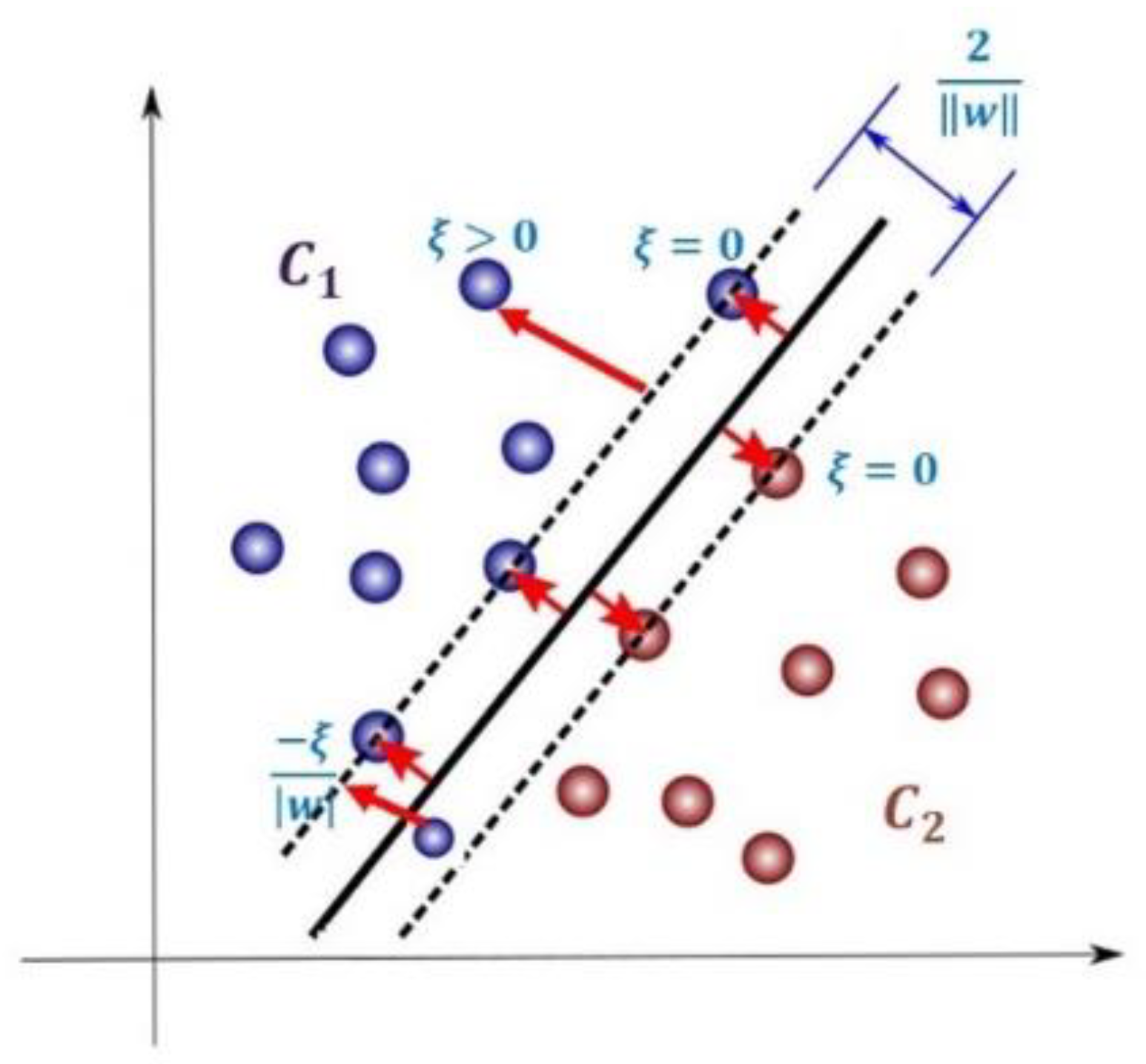
3.4.1. Support Vector Machine Classifier
Non-Separable Case
RBF SVMs
3.4.2. Gradient Boosted Trees:
3.5. Staging Melanocytic Neoplasms
4. Materials and Methods
4.1. Dataset
4.2. Hardware and Software Specifications
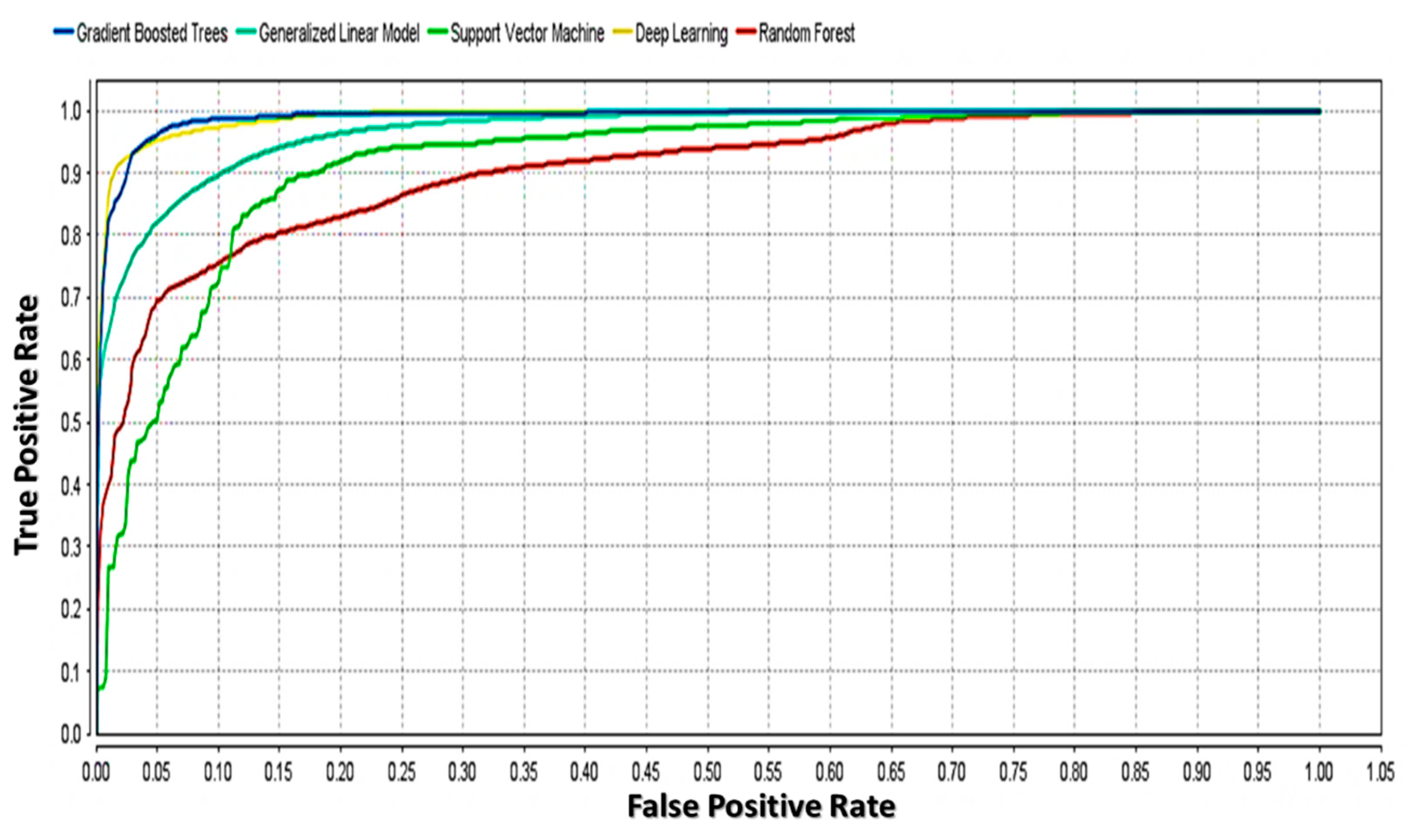
4.3. Performance Evaluation
4.4. Results
4.5. Discussion
5. Conclusions
Author Contributions
Funding
Conflicts of Interest
References
- Tschandl, P.; Wiesner, T. Advances in the diagnosis of pigmented skin lesions. Br. J. Dermatol. 2018, 178, 9–11. [Google Scholar] [CrossRef] [PubMed] [Green Version]
- Russo, T.; Piccolo, V.; Ferrara, G.; Agozzino, M.; Alfano, R.; Longo, C.; Argenziano, G. Dermoscopy pathology correlation in melanoma. J. Dermatol. 2017, 44, 507–514. [Google Scholar] [CrossRef] [PubMed]
- Jeffrey, G.; Danielle, S.; Orengo, I. Common Adult Skin and Soft Tissue Lesions. Semin Plast Surg. 2016, 30, 98–107. [Google Scholar]
- Ankad, B.S.; Sakhare, P.S.; Prabhu, M.H. Dermoscopy of non-melanocytic and pink tumors in brown skin: A descriptive study. Dermatopathol. Diagn. Dermatol. 2017, 4, 41–51. [Google Scholar] [CrossRef]
- Damsky, W.; Bosenberg, M. Melanocytic nevi and melanoma: Unraveling a complex relationship. HHS Public Access 2017, 36, 5771–5792. [Google Scholar] [CrossRef] [Green Version]
- Jason, P.; Lott, M. Almost one in Four Skin Biopsies is Melanocytic Proliferation; Medical Press: New Haven, CT, USA, 2017. [Google Scholar]
- Cannavò, S.P.; Tonacci, A.; Bertino, L.; Casciaro, M.; Borgia, F.; Gangemi, S.; Casciaro, M.; Borgia, F. The role of oxidative stress in the biology of melanoma: A systematic review. Pathol. Res. Pract. 2019, 215, 21–28. [Google Scholar] [CrossRef]
- Abbasi, N.R.; Shaw, H.M.; Rigel, D.S.; Friedman, R.J.; McCarthy, W.H.; Osman, I.; Kopf, A.W.; Polsky, D. Early Diagnosis of Cutaneous Melanoma. JAMA 2004, 292, 2771–2776. [Google Scholar] [CrossRef]
- Philip, C. Benign pigmented skin lesions. AJGP 2019, 48, 364–367. [Google Scholar]
- Kittler, H.; Marghoob, A.A.; Argenziano, G.; Carrera, C.; Curiel-Lewandrowski, C.; Hofmann-Wellenhof, R.; Malvehy, J.; Menzies, S.; Puig, S.; Rabinovitz, H.; et al. Standardization of terminology in dermoscopy/dermatoscopy: Results of the third consensus conference of the International Society of Dermoscopy. J. Am. Acad. Dermatol. 2016, 74, 1093–1106. [Google Scholar] [CrossRef] [Green Version]
- Khalil, A.; Elmogy, M.; Ghazal, M.; Burns, C.; El-Baz, A. Chronic Wound Healing Assessment System Based on Different Features Modalities and Non-Negative Matrix Factorization (NMF) Feature Reduction. IEEE Access 2019, 7, 80110–80121. [Google Scholar] [CrossRef]
- Anantha, M.; Moss, R.; Stoecker, W. Detection of pigment network in dermatoscopy images using texture analysis. Comput Med. Imaging Graph. 2011, 28, 225–234. [Google Scholar] [CrossRef] [PubMed] [Green Version]
- Abbes, W.; Sellami, D. Automatic Skin Lesions Classification Using Ontology-Based Semantic Analysis of Optical Standard Images. Procedia Comput. Sci. 2017, 112, 2096–2105. [Google Scholar] [CrossRef]
- Zaqout, I. Diagnosis of Skin Lesions Based on Dermoscopic Images Using Image Processing Techniques. In Pattern Recognition—Selected Methods and Applications; Intechopen Limited: London, UK, 2019. [Google Scholar] [CrossRef] [Green Version]
- Krig, S. Interest Point Detector and Feature Descriptor Survey. In Computer Vision Metrics; Apress: Berkeley, CA, USA, 2014. [Google Scholar]
- Krig, S. Global and Regional Features. In Computer Vision Metrics; Apress: Berkeley, CA, USA, 2014. [Google Scholar]
- Raju, S.; Rajan, E. Skin Texture Analysis Using Morphological Dilation and Erosion. Int. J. Pure Appl. Math. 2018, 118, 205–223. [Google Scholar]
- Olugbara, O.; Taiwo, T.; Heukelman, D. Segmentation of Melanoma Skin Lesion Using Perceptual Color Difference Saliency with Morphological Analysis. Math. Probl. Eng 2018. [Google Scholar] [CrossRef]
- Descombes, X.; Komech, S. Shape Descriptor Based on the Volume of Transformed Image Boundary. In Pattern Recognition and Machine Intelligence; Springer: Berlin, Germany, 2011; pp. 142–147. [Google Scholar]
- Amelard, R.; Wong, A.; Clausi, D. Extracting morphological high-level intuitive features (HLIF) for enhancing skin lesion classification. Conf Proc. IEEE Eng. Med. Biol Soc. 2012, 2012, 4458–4461. [Google Scholar]
- Ballerini, L.; Fisher, R.; Aldridg, B.; Rees, J.L. A Color and Texture Based Hierarchical K-NN Approach to the Classification of Non-melanoma Skin Lesions. In Color Medical Image Analysis; Springer Science: Berlin, Germany, 2013. [Google Scholar]
- Abbadi, N.; Faisal, Z. Detection and Analysis of Skin Cancer from Skin Lesions. Int. J. Appl. Eng. Res. 2017, 12, 9046–9052. [Google Scholar]
- Lynn, N.; War, N. Melanoma Classification on Dermoscopy Skin Images using Bag Tree Ensemble Classifier. In Proceedings of the International Conference on Advanced Information Technologies (ICAIT), Yangon, Myanmar, 6–7 November 2019. [Google Scholar]
- Ibraheem, M.R.; Elmogy, M. Automated Segmentation and Classification of Hepatocellular Carcinoma Using Fuzzy C-Means and SVM. In Medical Imaging in Clinical Applications, Studies in Computational Intelligence; Springer International Publishing: Cham, Switzerland, 2016. [Google Scholar]
- Moughal, T.A. Hyperspectral image classification using Support Vector Machine. J. Phys. Conf. Ser. 2013, 439. [Google Scholar] [CrossRef]
- Codella, N.C.F.; Gutman, D.; Celebi, M.E.; Helba, B.; Marchetti, M.A.; Dusza, S.W.; Kalloo, A.; Liopyris, K.; Mishra, N.; Kittler, H.; et al. Skin Lesion Analysis toward Melanoma Detection: A Challenge at the International Symposium on Biomedical Imaging (ISBI) 2016, hosted by the International Skin Imaging Collaboration (ISIC). arXiv 2016, arXiv:1605.01397. [Google Scholar]
- Do, T.-T.; Hoang, T.; Pomponiu, V.; Zhou, Y.; Chen, Z.; Cheung, N.-M.; Koh, D.; Tan, A.; Tan, S.-H.; Zhao, C.; et al. Accessible Melanoma Detection using Smartphones and Mobile Image Analysis. IEEE Trans. Multimed. 2018, 20, 2849–2864. [Google Scholar] [CrossRef] [Green Version]
- Lee, Y.; Jung, S.; Won, H. WonDerM: Skin Lesion Classification with Fine-tuned Neural Networks. Available online: https://arxiv.org/abs/1808.03426 (accessed on 3 September 2020).
- Nammalwar, P.; Ghita, O.; Whelan, P. Integration of Colour and Texture Distributions for Skin Cancer Image Segmentation. Available online: https://www.researchgate.net/publication/236645646_Integration_of_Colour_and_Texture_Distributions_for_Skin_Cancer_Image_Segmentation (accessed on 3 September 2020).
- Codella, N.C.F.; Nguyen, Q.-B.; Pankanti, S.; Gutman, D.; Helba, B.; Halpern, A.C.; Smith, J.R. Deep learning ensembles for melanoma recognition in dermoscopy images. IBM J. Res. Dev. USA 2017, 6, 4–5. [Google Scholar] [CrossRef] [Green Version]
- Li, Y.; Shen, L. Skin Lesion Analysis towards Melanoma Detection Using Deep Learning Network. Sensors 2018, 18, 556. [Google Scholar] [CrossRef] [PubMed] [Green Version]
- Kawahara, J.; BenTaieb, A.; Hamarneh, G. Deep features to classify skin lesions. In International Symposium on Biomedical Imaging (ISBI); IEEE: Prague, Czech Republic, 2016. [Google Scholar]
- Shrestha, B.; Bishop, J.; Kam, K.; Chen, X.; Moss, R.H.; Stoecker, W.V.; Umbaugh, S.; Stanley, R.J.; Celebi, M.E.; Marghoob, A.A.; et al. detection of atypical texture features in early malignant melanoma. Ski. Res. Technol. 2010, 16, 60–65. [Google Scholar] [CrossRef] [PubMed] [Green Version]
- Ganster, H.; Pinz, A.; Röhrer, R. Automated Melanoma Recognition. IEEE Trans. ON Med Imaging 2001, 20, 233–239. [Google Scholar] [CrossRef] [PubMed]
- Rezvantalab, A.; Safigholi, H.; Karimijeshni, S. Dermatologist Level Dermoscopy Skin Cancer Classification Using Different Deep Learning Convolutional Neural Networks Algorithms. Comput. Vis. Pattern Recognit. arXiv 2018, arXiv:1810.10348. [Google Scholar]
- Hekler, A.; Utikal, J.S.; Enk, A.H.; Hauschild, A.; Weichenthal, M.; Maron, R.C.; Berking, C.; Haferkamp, S.; Klode, J.; Schadendorf, D.; et al. Superior skin cancer classification by the combination of human and artificial intelligence. Eur. J. Cancer 2019, 120, 114–121. [Google Scholar] [CrossRef] [Green Version]
- Adekanmi, A.; Viriri, S. Deep Learning-Based System for Automatic Melanoma Detection. IEEE Access 2020, 8, 7160–7172. [Google Scholar]
- Phillips, M.; Greenhalgh, J.; Marsden, H.; Palamaras, L. Detection of Malignant Melanoma Using Artificial Intelligence: An Observational Study of Diagnostic Accuracy. Dermatol. Pract. Concept. 2020, 10, e2020011. [Google Scholar]
- Michael Phillips, M.; Marsden, H.; Jaffe, W.; Matin, R.N.; Wali, G.N.; Greenhalgh, J.; McGrath, E.; James, R.; Ladoyanni, E.; Bewley, B.; et al. Assessment of Accuracy of an Artificial Intelligence Algorithm to Detect Melanoma in Images of Skin Lesions. JAMA Netw. Open 2019, 2, e1913436. [Google Scholar] [CrossRef] [Green Version]
- Haenssle, H.A.; Fink, C.; Schneiderbauer, R.; Toberer, F.; Buhl, T.; Blum, A.; Kalloo, A.; Hassen, A.B.H.; Thomas, L.; Enk, A.; et al. Man against machine: Diagnostic performance of a deep learning convolutional neural network for dermoscopic melanoma recognition in comparison to 58 dermatologists. Ann. Oncol. 2018, 29, 1836–1842. [Google Scholar] [CrossRef]
- Verma, A.; Pal, S.; Kumarb, S. Comparison of skin disease prediction by feature selection using ensemble data mining techniques. Inform. Med. Unlocked 2019, 16, 100202. [Google Scholar] [CrossRef]
- Hoshyar, A.N.; Al-Jumailya, A.; Hoshyar, A.N. The Beneficial Techniques in Pre-processing Step of Skin Cancer Detection System Comparing. In Procedia Computer Science; Elsevier: Amsterdam, The Nertherlands, 2014; pp. 25–31. [Google Scholar]
- Campos, G.; Mastelini, S.; Aguiar, G. Machine learning hyperparameter selection for Contrast Limited Adaptive Histogram Equalization. EURASIP J. Image Video Process. 2019, 59. [Google Scholar] [CrossRef] [Green Version]
- Krig, S. Local Feature Design Concepts, Classification, and Learning. In Computer Vision Metrics; Apress: Berkeley, CA, USA, 2014. [Google Scholar]
- Iwanowski, M. Morphological Boundary Pixel Classification. In Proceedings of the International Conference on “Computer as a Tool”, Warsaw, Poland, 9–12 September 2007. [Google Scholar]
- Ramkumar, P. Morphological Representation Operators, Algorithms And Shape Descriptors. Available online: https://shodhganga.inflibnet.ac.in/bitstream/10603/40771/8/08_chapter3.pdf (accessed on 3 September 2020).
- Banerjee, S.; Sahasrabudhe, S. A morphological shape descriptor. J. Math. Imaging Vis. 1994, 4, 43–55. [Google Scholar] [CrossRef]
- Zhang, L.; Dong, W.; Zhang, D.; Shi, G. Two-stage image denoising by principal component analysis with local pixel grouping. Pattern Recognit. 2010, 43, 1531–1549. [Google Scholar] [CrossRef] [Green Version]
- Cao, H.; Naito, T.; Ninomiya, Y. Approximate RBF Kernel SVM and Its Applications in Pedestrian Classification. Available online: https://www.researchgate.net/publication/29621872_Approximate_RBF_Kernel_SVM_and_Its_Applications_in_Pedestrian_Classification (accessed on 3 September 2020).
- Afentoulis, V.; Lioufi, K. Svm Classification With Linear And Rbf Kernels. Available online: https://www.researchgate.net/publication/279913074_SVM_Classification_with_Linear_and_RBF_kernels (accessed on 3 September 2020).
- Song, B.; Sacan, A. Automated wound identification system based on image segmentation and artificial neural networks. In Proceedings of the 2012 IEEE International Conference on Bioinformatics and Biomedicine, Philadelphia, PA, USA, 4–7 October 2012; pp. 1–4. [Google Scholar]
- Liu, S.; Xiao, J.; Liu, J.; Wang, X.; Wu, J.; Zhu, J. Visual Diagnosis of Tree Boosting Methods. IEEE Trans. Vis. Comput. Graph. 2018, 24, 163–173. [Google Scholar] [CrossRef] [Green Version]
- Yang, J. Applying Boosting Algorithm for Improving Diagnosis of Interstitial Lung Diseases. Available online: http://cs229.stanford.edu/proj2016/report/YangApplyingBoostingAlgorithmForImprovingDiagnosisOfInterstitialLungDisease-report.pdf (accessed on 3 September 2020).
- Friedman, J.H. Machine. Ann. Stat. 2001, 29, 1189–1232. [Google Scholar] [CrossRef]
- Jiménez, A.; Serrano, C.; Acha, B.; Karray, F.; Campilho, A.; Cheriet, F. Automatic Detection of Globules, Streaks and Pigment Network Based on Texture and Color Analysis in Dermoscopic Images. In Bioinformatics Research and Applications; Springer Science: Berlin, Germany, 2017; pp. 486–493. [Google Scholar]
- PH2 Dataset. Available online: https://www.fc.up.pt/addi/ph2%20database.html (accessed on 3 September 2020).
- Bradley, P.; Andrew, P. The use of the area under the ROC curve in the evaluation of machine learning algorithms. Pattern Recognit 1997, 30, 1145–1159. [Google Scholar] [CrossRef] [Green Version]


| Study | Image Analysis | Dataset | Methodology | Performance |
|---|---|---|---|---|
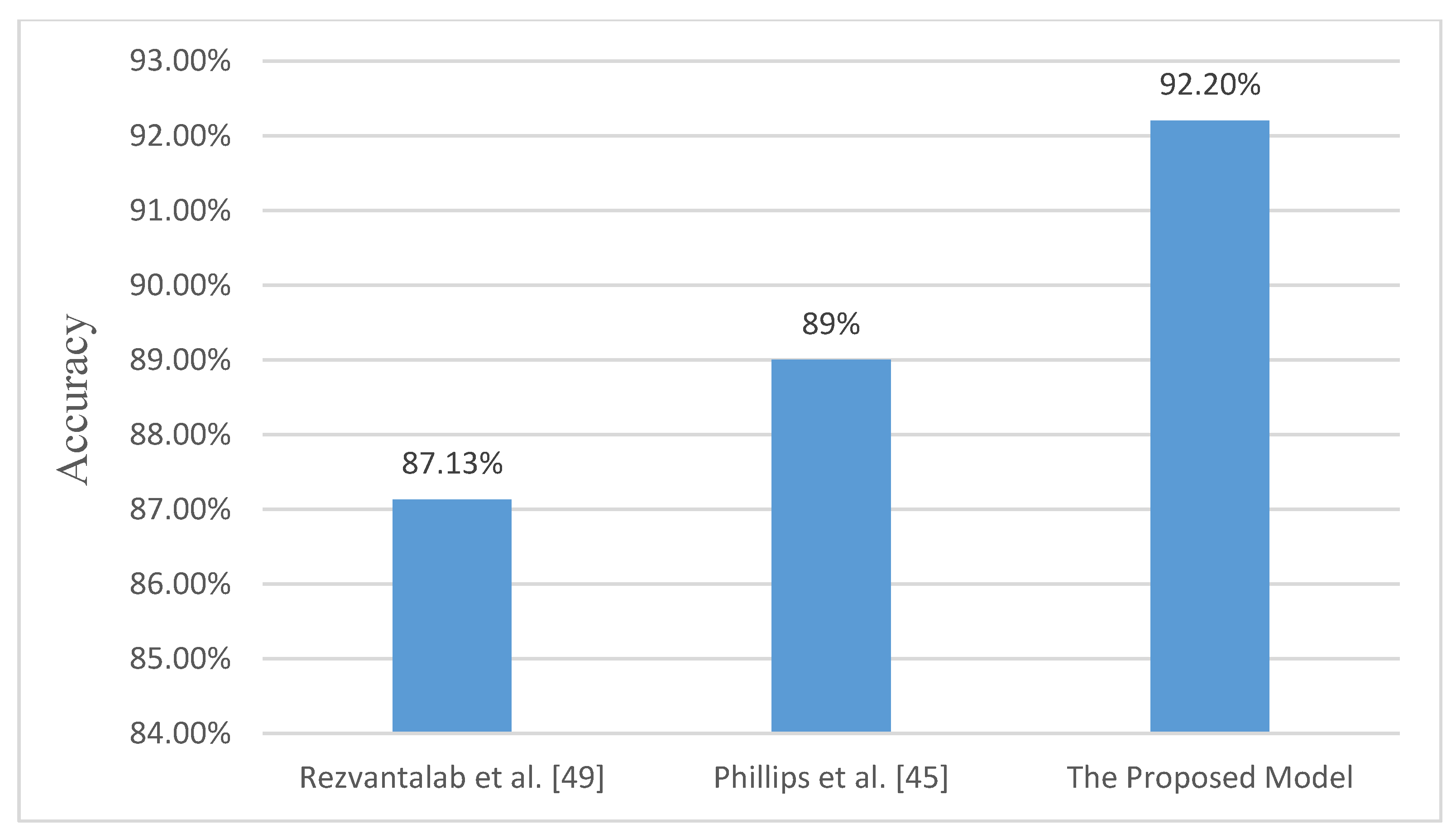
| Rezvantalab et al. [35] | Classification of 8 diagnostic categories of skin diseases | 120 images PH2 dataset and 10,015 HAM10000 | 4 deep convolutional neural networks | Average Accuracy 87.13% |
| Hekler et al. [36] | Classification of skin lesions images into five diagnostic categories | 300 images HAM10000 (60 for each disease class | Convolutional neural networks (CNN) into a binary output | Accuracy 82.95% |
| Adekanmi and Viriri [37] | Classification of melanoma lesions | PH2 dataset | Softmax classifier for pixel-wise | Accuracy 95% (Binary output classifier) |
| Lynn and War [23] | Skin lesion border detection system | ISBI2016, ISIC2017, PH2 datasets | Asymmetry, border, color, and diameter (ABCD) feature extraction rule and bagging decision tree ensemble classifier | Average accuracy 84.5% |
| Gutman et al. [26] | Automatic detection for globules and streaks | 807 training and 335 testing form ISIC 2016 dataset | Superpixels feature extraction mask in addition to dermoscopic features | Accuracy 91% |
| Abbadi and Faisal [22] | Detecting and segmenting malignant and benign lesion image | 220 images: 120 from PH2 and 100 from the websites | YUV color space conversion, ABCD rules, segmentation based on Markov and Laplace filter | Accuracy 95.45% (Binary output classifier) |
| Lee et al. [28] | WonDerM pipeline (pre-processing, segmentation and classification) | HAM10000 Dataset | (DenseNet and U-net) | Accuracy 89.9% |
| Do et al. [27] | Detection of melanoma | 117 benign nevi and 67 malignant melanomas | GLCM features, hierarchical segmentation and SVM classifier | Specificity 90% |
| Nammalwar et al. [29] | Segmentation of skin lesions | 18 images | ABCD’s clinical features, Modified Kolmogorov–Smirnov (MKS), boundary refinement algorithm | Figure comparisons |
| Codella et al. [30] | Segmentation and classification of melanoma | ISBI 2016 dataset | U-Net architecture, six color channels, RGB (red, green, and blue) and HSV (hue, saturation, and value) color spaces | Accuracy 76% |
| Li and Shen [31] | Segmentation, feature extraction, and lesion classification using two deep learning methods | ISBI 2016 dataset 2000 images | two fully convolutional residual networks (FCRN), lesion index calculation unit (LICU) | Accuracy 83.3% |
| Kawahara et al. [23] | Linear classifier with no lesion segmentations nor pre-processing | 1300 images | multi-scale features using CNN | Accuracy 81.8% |
| Ballerini et al. [21] | Hierarchical classifier | 960 images | k-nearest neighbors, region-based active contour | Accuracy 74% |
| Shrestha et al. [33] | Discrimination of early malignant melanoma | 106 images | Haralick statistical texture measures | Accuracy 95.4% |
| Ganster et al. [34] | Early recognition of melanoma | 5393 images | shape, color and local features, k-nearest neighbor (KNN) classifier | Accuracy 88% |
| Phillips et al. [38] | Recognition of Melanoma | 7102 dermoscopic images | Deep Ensemble Model | Area under the curve (AUC) of 0.93, 85% for sensitivity |
| Phillips et al. [39] | Assessment of the suspicious from benign skin lesions | 1550 images | artificial intelligence algorithm | AUC of 90.1% for biopsied lesions and 95.8% for other lesions |
| Haenssle et al. [40] | Detection of melanoma | Compared to an international group of 58 dermatologists. | CNN | 82.5%, sensitivities of 86.6% and 88.9% AUC |
| Start Load the training data Load the corresponding GT data Load the labels CSV file Step 1. Pre-processing: Step 1.1 Image resize: Images were rescaled to 768 × 576 Step 1.2 Image Enhancement: Images were enhanced using CLAHE. Step 1.3 Image Conversion: Images were converted to grayscale. Step 2. Pixel base Segmentation: For Original Color Images For Corresponding GT Images For CSV labels file Test whether a label is melcyt nv, dysp nv or mel Use Corresponding GT mask along with Original Color Images End for Return single pixel labels have the values {0; 1; 2; 3}; 0 for background, 1 for melcyt nv lesion, 2 for dysp nv and 3 for mel Save integer intensity levels array of segmented images as labels mat file. End |
| Classifier | Parameters | Value |
|---|---|---|
| SVM | Kernel | RBF |
| Gamma | 0.01 | |
| C parameter | 1000 | |
| Support vectors | 1176 | |
| Bias (offset) | 1.234 | |
| GBT | No. of trees | 150 |
| Maximal depth | 7 | |
| Learning rate | 0.1 | |
| RF | No. of decision trees | 140 |
| Maximal depth | 7 | |
| NB | NB model | Bayesian |
| Distribution best-fit | Gaussian | |
| Distribution type | multinomial | |
| DL | No. of epochs | 20 |
| Activation function | ReLU | |
| Loss function | Cross-Entropy | |
| 𝜖 | 1.0 × 10⁻⁸ | |
| L1 | 1.0 × 10⁻⁵ | |
| L2 | 0 |
| Model | ACC | AUC | DSC | Sen | Spec | Recall | Precision | Total Time |
|---|---|---|---|---|---|---|---|---|
| SVM | 92.2% ± 0.3 | 0.969 ± 0.012 | 95.1% ± 0.2 | 99.0% ± 0.2 | 69.9% ± 5.3 | 99.0% ± 0.2 | 91.5% ± 0.3 | 25 min, 55 s |
| GBT | 92.1% ± 0.1 | 0.962 ± 0.002 | 95.0% ± 0.1 | 98.5% ± 0.1 | 71.1% ± 0.8 | 98.5% ± 0.1 | 91.8% ± 0.2 | 12 min, 40 s |
| RF | 90.0% ± 0.2 | 0.945 ± 0.003 | 93.6% ± 0.1 | 95.4% ± 0.3 | 72.5% ± 0.9 | 95.4% ± 0.3 | 91.9% ± 0.2 | 20 min, 53 s |
| NB | 84.7% ± 0.0 | 0.906 ± 0.0 | 89.9% ± 0.0 | 89.1% ± 0.0 | 70.1% ± 0.2 | 89.1% ± 0.0 | 90.7% ± 0.0 | 6 min, 1 s |
| DL | 84.1% ± 0.1 | 0.898 ± 0.0 | 90.5% ± 0.1 | 98.9% ± 0.0 | 35.8% ± 0.5 | 98.9% ± 0.0 | 83.5% ± 0.1 | 8 min, 39 s |
| Model | ACC | AUC | DSC | Sen | Spec | Recall | Precision | Total Time |
|---|---|---|---|---|---|---|---|---|
| SVM | 92.9% ± 0.3 | 0.959 ± 0.007 | 95.3% ± 0.2 | 98.8% ± 0.1 | 86.7% ± 1.5 | 98.8% ± 0.1 | 94.8% ± 0.6 | 16 min, 22 s |
| GBT | 91.6% ± 0.4 | 0.959 ± 0.001 | 94.2% ± 0.3 | 93.5% ± 0.9 | 77.5% ± 0.6 | 93.5% ± 0.9 | 92.0% ± 0.5 | 11 min, 14 s |
| RF | 89.8% ± 0.4 | 0.945 ± 0.002 | 92.9% ± 0.2 | 92.6% ± 0.3 | 82.6% ± 1.0 | 92.6% ± 0.3 | 93.3% ± 0.4 | 15 min, 15 s |
| NB | 85.2% ± 0.1 | 0.923 ± 0.0 | 89.2% ± 0.0 | 84.8% ± 0.0 | 86.4% ± 0.2 | 84.8% ± 0.1 | 94.2% ± 0.1 | 4 min, 13 s |
| DL | 90.1% ± 0.1 | 0.956 ± 0.002 | 93.6% ± 0.0 | 99.9% ± 0.0 | 64.8% ± 0.3 | 99.9% ± 0.0 | 88.0% ± 0.1 | 7 min, 35 s |
© 2020 by the authors. Licensee MDPI, Basel, Switzerland. This article is an open access article distributed under the terms and conditions of the Creative Commons Attribution (CC BY) license (http://creativecommons.org/licenses/by/4.0/).
Share and Cite
Ibraheem, M.R.; El-Sappagh, S.; Abuhmed, T.; Elmogy, M. Staging Melanocytic Skin Neoplasms Using High-Level Pixel-Based Features. Electronics 2020, 9, 1443. https://doi.org/10.3390/electronics9091443
Ibraheem MR, El-Sappagh S, Abuhmed T, Elmogy M. Staging Melanocytic Skin Neoplasms Using High-Level Pixel-Based Features. Electronics. 2020; 9(9):1443. https://doi.org/10.3390/electronics9091443
Chicago/Turabian StyleIbraheem, Mai Ramadan, Shaker El-Sappagh, Tamer Abuhmed, and Mohammed Elmogy. 2020. "Staging Melanocytic Skin Neoplasms Using High-Level Pixel-Based Features" Electronics 9, no. 9: 1443. https://doi.org/10.3390/electronics9091443
APA StyleIbraheem, M. R., El-Sappagh, S., Abuhmed, T., & Elmogy, M. (2020). Staging Melanocytic Skin Neoplasms Using High-Level Pixel-Based Features. Electronics, 9(9), 1443. https://doi.org/10.3390/electronics9091443