1. Introduction
In recent years, with the escalating energy crisis and environmental problems, low-pollution, high-efficiency electric vehicles (EVs) have become a hot spot in the automotive industry. Lithium-ion batteries have the characteristics of small size, light weight, high energy density, large output power and high safety performance, and have become the first choice for energy storage devices of EVs [
1,
2,
3]. State of charge (SOC) is used to directly reflect the remaining capacity of the battery, which is an important basis for the vehicle control system to formulate an optimal energy management strategy. SOC is an important battery performance parameter; accurate estimation of SOC is of great significance to improve battery safety performance, extend battery life and ensure reliable operation of battery system [
4,
5].
At present, the commonly used SOC estimation methods for lithium batteries include the ampere-hour integration method, the open circuit voltage method, the neural network method, the particle filter algorithm and the Kalman Filter (KF) method. Among them, the ampere-hour integration method estimates the SOC of the battery by accumulating the amounts of charge and discharge, and at the same time compensates the estimated SOC according to the self-discharge rate [
6,
7]. The ampere-hour integration method is relatively simple; it can dynamically estimate the battery SOC, but the current integration needs to obtain the initial SOC value, and the battery current must be accurately collected, which leads to the accumulation of SOC estimation errors over time. In practical applications, the ampere-hour integration method is usually used in combination with other methods to improve the estimation accuracy.
The open circuit voltage method is to indirectly fit the corresponding relationship between the open circuit voltage and the battery SOC, according to the relationship between the open circuit voltage of the battery and the lithium ion concentration in the battery [
8,
9]. The open circuit voltage method requires the battery to be placed statically for a long time to obtain a stable terminal voltage. Therefore, the open circuit voltage method cannot be used to estimate the SOC of the battery online in real time.
The neural network method is an algorithm for simulating the human brain and its neurons to deal with nonlinear systems, without in-depth study of the internal structure of the battery. The neural network method only needs to extract a large number of input and output samples from the target battery in accordance with its working characteristics in advance, and input it into the system established by using this method, and the SOC of the battery can be obtained [
10,
11]. The neural network method has high operational complexity, and it needs to extract a large amount of comprehensive target sample data to train the system. The input training data and training method will affect the accuracy of SOC estimation to a large extent.
The particle filtering is a process of approximating the probability density function by finding a set of random samples propagating in the state space, replacing the integral operation with the sample mean and then obtaining the minimum variance estimation process of the system state [
12,
13]. The particle filter algorithm is suitable for nonlinear non-Gaussian systems. The more particles used, the more accurate the SOC estimation value. However, as the number of particles increases, the calculation load increases. Additionally, particle degradation and insufficient particle diversity will seriously affect the SOC estimation results.
The KF algorithm is a type of optimized autoregressive data filtering algorithm. The essence of the algorithm is to make an optimal estimate of complex dynamic systems according to the principle of least mean square error [
14,
15,
16,
17,
18]. KF algorithm overcomes the serious shortcoming of the current integration dependence on the initial value, and does not require a large number of sample data, and can be used to estimate the battery SOC online. In the SOC estimation of electric vehicle power batteries with complex operating conditions, the KF algorithm has a significant application value, and has become a hot spot in the research of battery SOC estimation algorithms in recent years [
19,
20]. The KF is an algorithm that uses the linear system state equation to observe the system input and output data to optimally estimate the state of the system.
Since KF cannot solve the problem of nonlinear systems, study [
21] used the extended Kalman filter (EKF) to expand nonlinear systems into linear systems using Taylor series. EKF is an extended form of the standard Kalman filter in non-linear situations, and it is a highly efficient recursive filter. The basic idea of EKF is to use Taylor series expansion to linearize the nonlinear system, and then use the Kalman filter framework to filter the signal, so it is a sub-optimal filter. EKF algorithm is used for SOC estimation in battery management systems (BMSs), and has achieved good results in SOC estimation based on equivalent circuit model [
22,
23,
24]. Although this method solves the nonlinear problem, it ignores high-order terms and increases linear errors, which may cause the filter to diverge.
Reference [
25] used the unscented Kalman filter (UKF) to perform an unscented transformation on a nonlinear system without ignoring higher-order terms, which improved the accuracy of the estimation. UKF is a combination of unscented transform and standard Kalman filter system. Through unscented transform, the nonlinear system equation is suitable for the standard Kalman system under the linear assumption. The basic idea of UKF is Kalman filtering and unscented transform, which can effectively overcome the problems of low accuracy and poor stability of EKF estimation. As high-order terms are not ignored, the calculation accuracy of nonlinear distribution statistics is high. However, the uncertainty of the battery model and system noise is not considered. Uncertainty of model noise and system noise will lead to increased error, slow convergence speed and filter divergence. Reference [
26] introduces adaptive filtering on the basis of UKF, and replaces system noise covariance and observation noise covariance of UKF with adaptive-filter-estimated system noise covariance and observation noise covariance, respectively. In order to update the system error and the observation error in real time, the filtering effect is relatively good, but the adaptive filtering cannot truly reflect the system noise and the observation noise error, so it can be further improved.
In the traditional UKF algorithm [
27,
28], the system noise covariance and the observation noise covariance are usually set as constants, which cannot truly reflect the dynamic characteristics of noise, and have a certain influence on the accuracy of SOC estimation. In view of the shortcomings of the traditional UKF algorithm in the case of low model accuracy and uncertain noise, we designed an adaptive unscented Kalman filter (AUKF). The AUKF algorithm monitors the dynamic changes of innovation and residual in the filter in real time; corrects the system noise covariance and observation noise covariance in real time; and adjusts the filter gain to improve the estimation accuracy.
The organizational structure of this paper is as follows. In
Section 1, the common methods for battery SOC estimation are introduced, and the methods designed in this paper are briefly introduced. In
Section 2, the second-order RC equivalent circuit model is established, the parameters are identified and the accuracy of the model is verified. In
Section 3, the traditional UKF algorithm and the AUKF algorithm designed in this paper are introduced. In
Section 4, the convergence speed and estimation accuracy of the UKF algorithm and AUKF algorithm are compared through experiments. In
Section 5, the work and research results of this paper are summarized.
3. Design of the SOC Estimation Algorithm
For a nonlinear system, the state equation and observation equation considering the system noise and observation noise are as shown in Equation (12):
where
is the current moment,
is the nonlinear system state transition equation,
is the nonlinear observation equation,
is the state variable,
is the known input,
is the observation signal,
is the system noise and
is the observation noise.
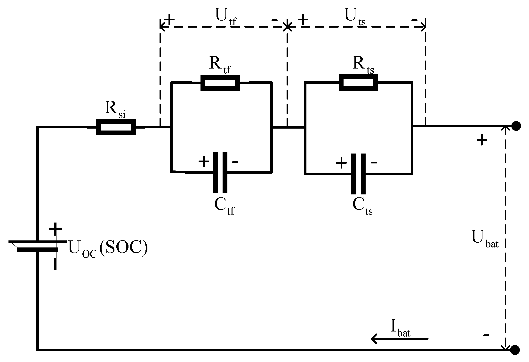
According to the second-order equivalent circuit model of the battery, combining Equations (1) and (2), the discretized state equation and observation equation of the equivalent circuit model of the battery can be shown in Equation (13):
Equations (13) can be simplified to Equations (14):
where
, , , is the ohmic internal resistance of the battery.
According to the KF principle, combining Equations (12) and (14), the first derivative of the nonlinear observation equation is calculated at the current state value, and the observation matrix can be obtained as Equation (15).
3.1. Design of the Unscented Kalman Filter Algorithm
The unscented Kalman filter (UKF) is a combination of the unscented transform (UT) and the standard Kalman filter system, and uses the unscented transform to adapt the nonlinear system equations to the standard Kalman system under the linear assumption. UKF uses statistical linearization technology, which mainly linearizes the nonlinear function of random variables through linear regression of n Sigma points collected in the prior distribution. This linearization is more accurate than Taylor series linearization. The basic idea of UKF is Kalman filtering and unscented transform. Since UKF does not ignore high-order terms, it can effectively overcome the problems of low accuracy and poor stability of EKF estimation.
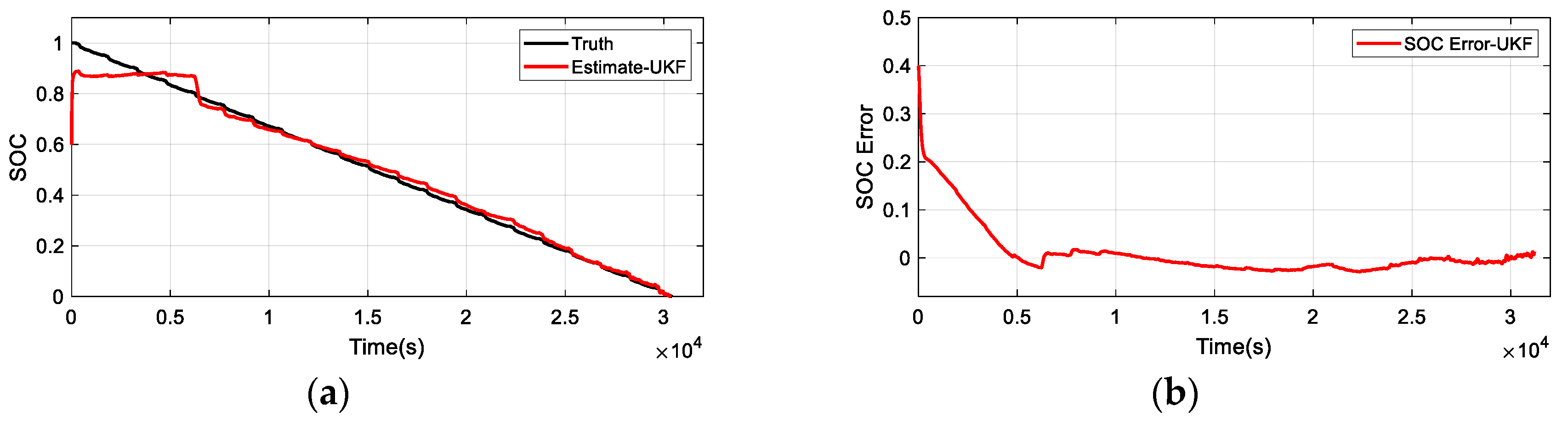
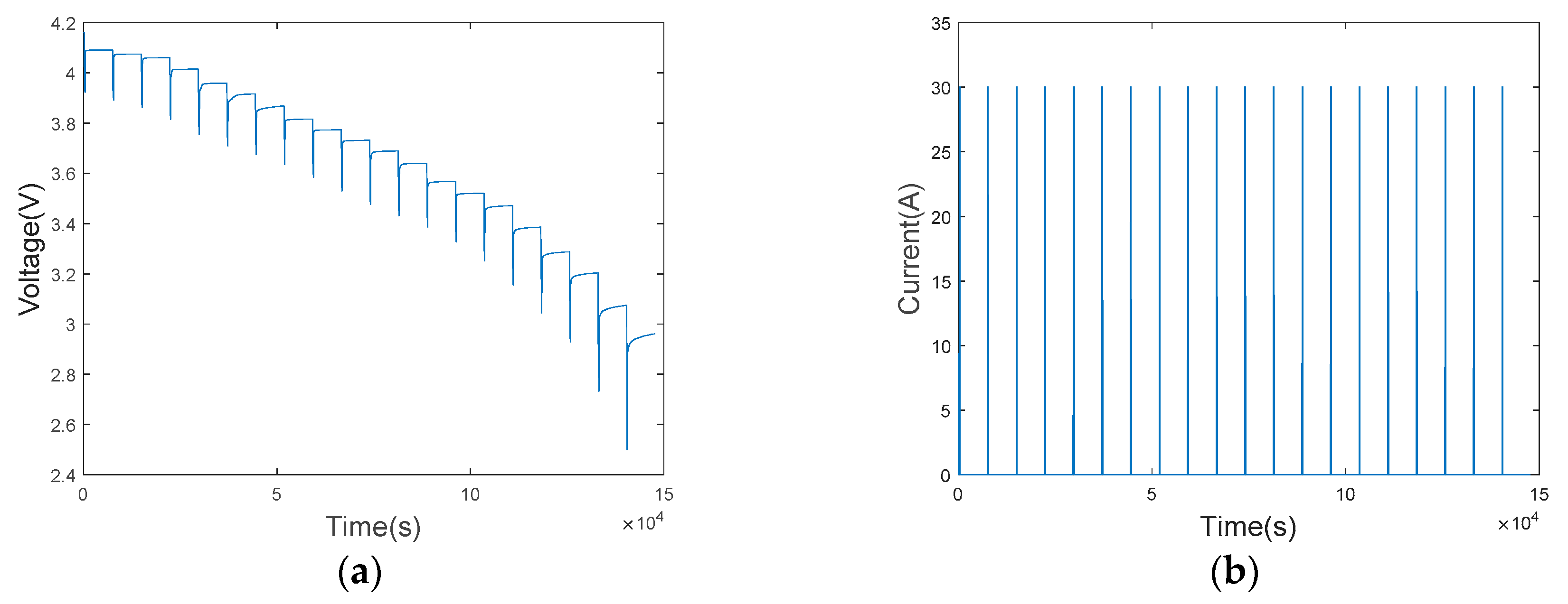
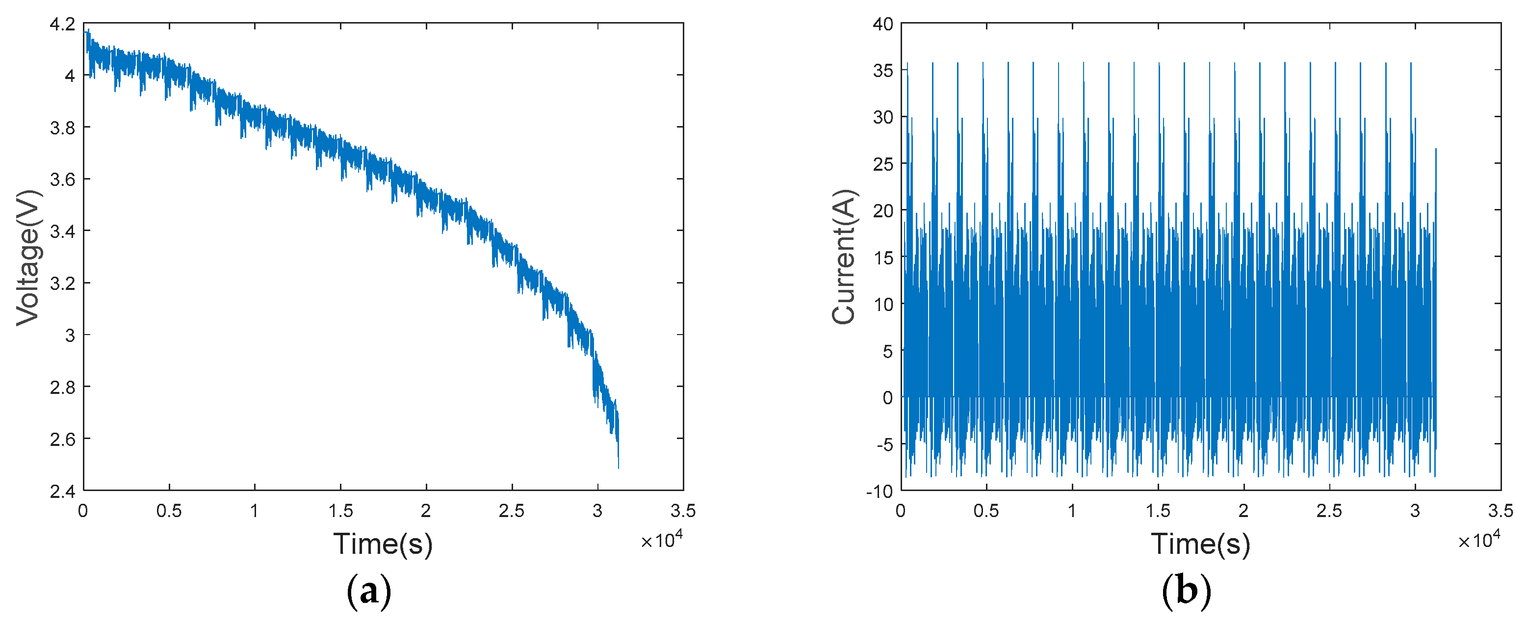
We conducted simulation experiments in MATLAB, and used the UKF algorithm to perform SOC estimation experiments under urban dynamometer driving schedule (UDDS) conditions, where the initial value , .
The UDDS operating conditions are shown in
Figure 8. The estimation terminal voltage of the battery using the UKF algorithm for SOC estimation is shown in
Figure 9. The SOC estimation results of the battery using the UKF algorithm for SOC estimation are shown in
Figure 10.
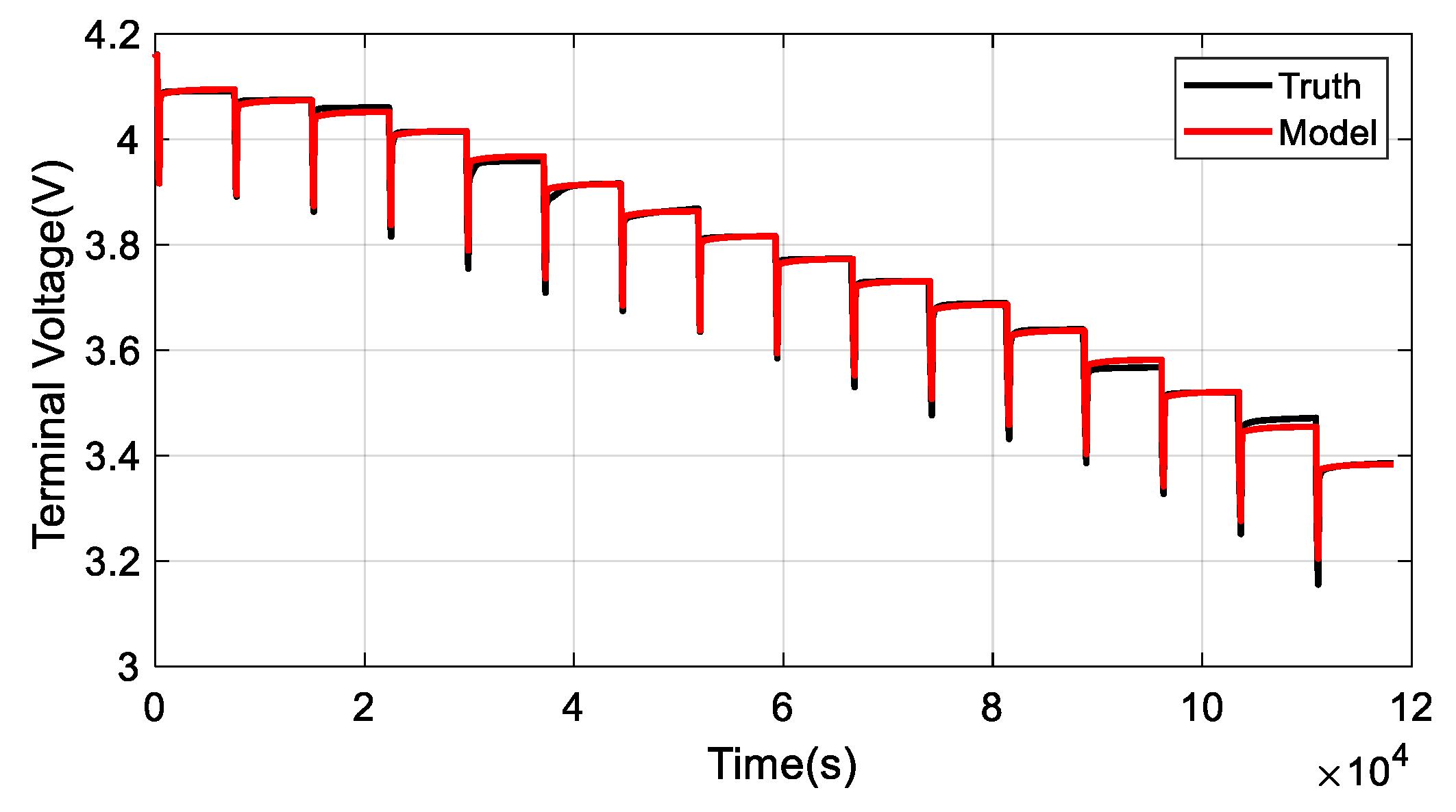
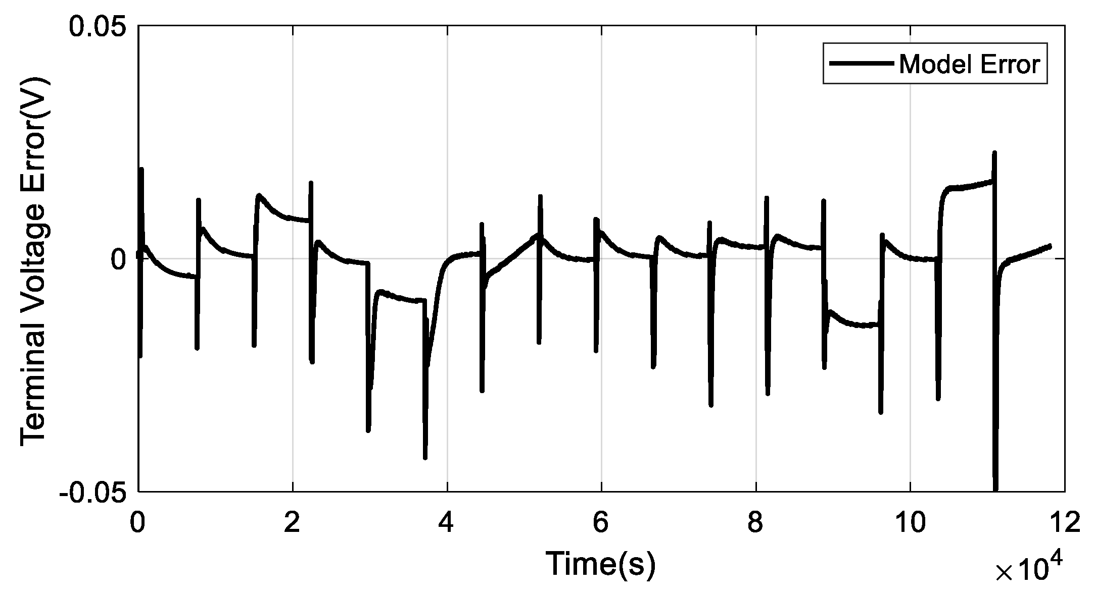
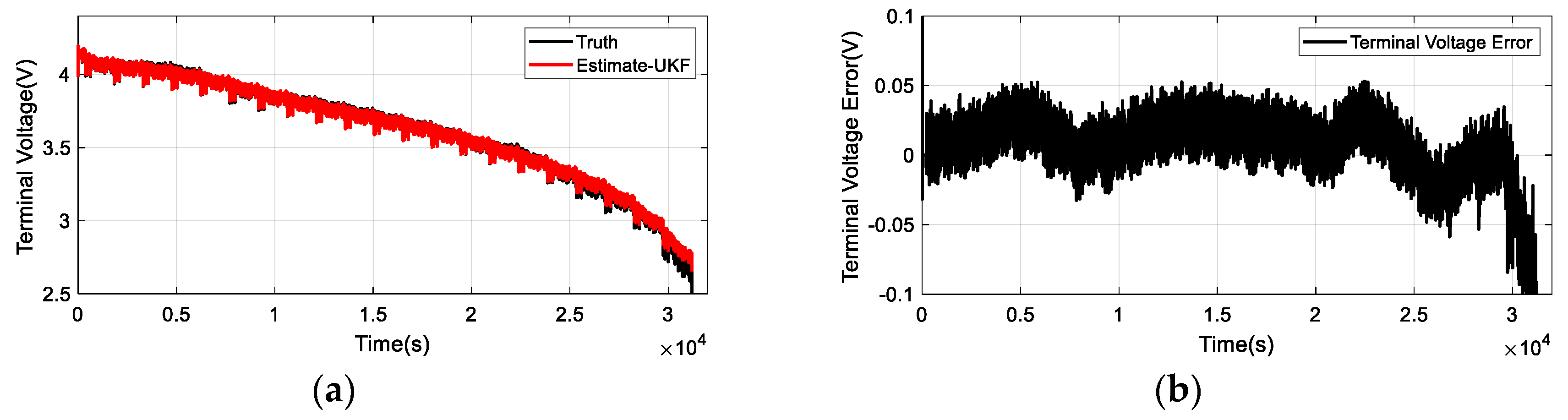
In
Figure 9, the battery terminal voltage estimated by the UKF algorithm is shown. In
Figure 9a, the estimated terminal voltage is compared with the true terminal voltage, and the estimated terminal voltage is not much different from the true terminal voltage. In
Figure 9b, the terminal voltage error value of the battery fluctuates greatly. In
Figure 10, the SOC of the battery estimated by UKF is shown. In
Figure 10a, the estimated SOC of the battery differs greatly from the true value before 5000 seconds. In
Figure 10b, the SOC estimation error of the battery just approached zero after 5000 seconds, and the convergence speed of the filter is slow.
3.2. Design of the Adaptive Unscented Kalman Filter Algorithm
The UKF algorithm uses UT to replace Taylor series expansion to transform a nonlinear system into a linear system, improving the accuracy of the algorithm. However, in the UKF algorithm, the system model noise and observation noise are set as constants, which cannot reflect the effect of real noise on the filter, which causes the SOC estimation error to increase or even diverge. In order to solve the above problems, we designed an AUKF algorithm; the algorithm is improved on the basis of the UKF algorithm; the algorithm monitors the change of innovation and residual in the filter in real time, and calculates the variance of innovation and residual by the moving window method. The system noise covariance is corrected in real time by the innovation variance, and the observation noise covariance is corrected in real time by the residual variance.
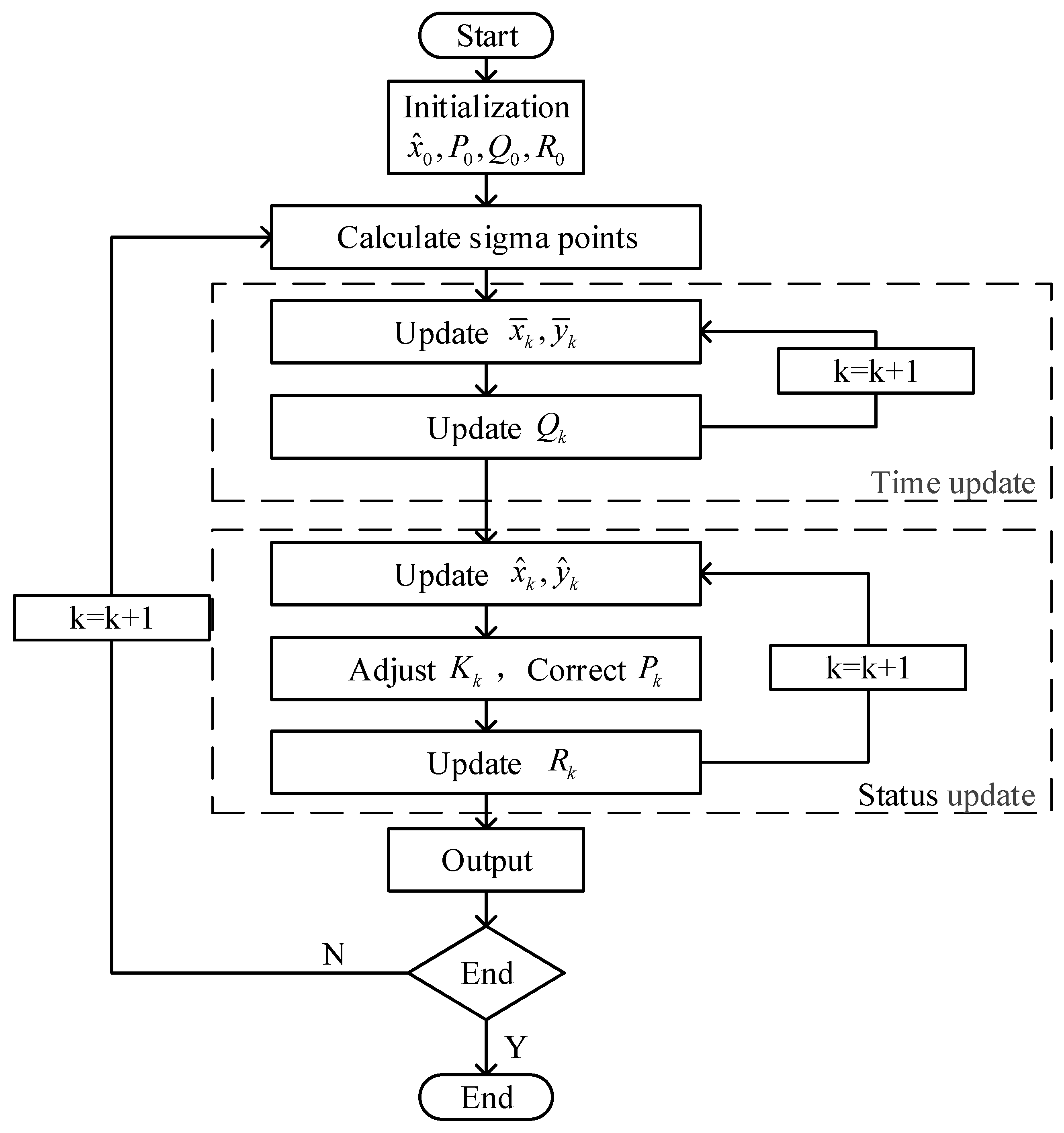
The AUKF algorithm process is as follows:
(1) Determine the initial value of state value
and the initial value of state error covariance
:
(2) Calculate Sigma point:
where
is the length of the state vector, the length of the state vector in this paper is 3 and the weight value calculation is shown in Equation (19):
where
.
(3) Time update.
Update predicted status value
:
Update predicted observation
.
Update system covariance prediction value
.
Calculate innovation value
and innovation variance value
.
Update system noise covariance
.
(4) Status update.
Update observation covariance prediction value
.
Update covariance
.
Calculate Kalman gain
.
Update estimated state value
.
Update estimated observation
.
Update error covariance
.
Calculate the residual value
and the residual variance value
.
Update the observation noise covariance
.
The AUKF algorithm flow is shown in
Figure 11.
3.2.1. Adaptive System Noise Covariance
From Equations (18), (21), (24), (27) and (33), it can be seen that when the value is too large, system covariance prediction increases, so that the next predicted state value becomes larger, which eventually leads to the estimated state value being too large, which increases the SOC estimation error. Therefore, the system noise covariance can be updated in real time to correct the influence of the system error on the estimation result.
The innovation
at time
is defined as the difference between the actual observation value
and the predicted observation value
. The expression of innovation is shown in Equation (37):
According to the moving window method, the variance of innovation
is calculated as:
where
is the length of the moving window. Through the innovation variance
, the system noise covariance
can be calculated [
36] as shown in Equation (39),
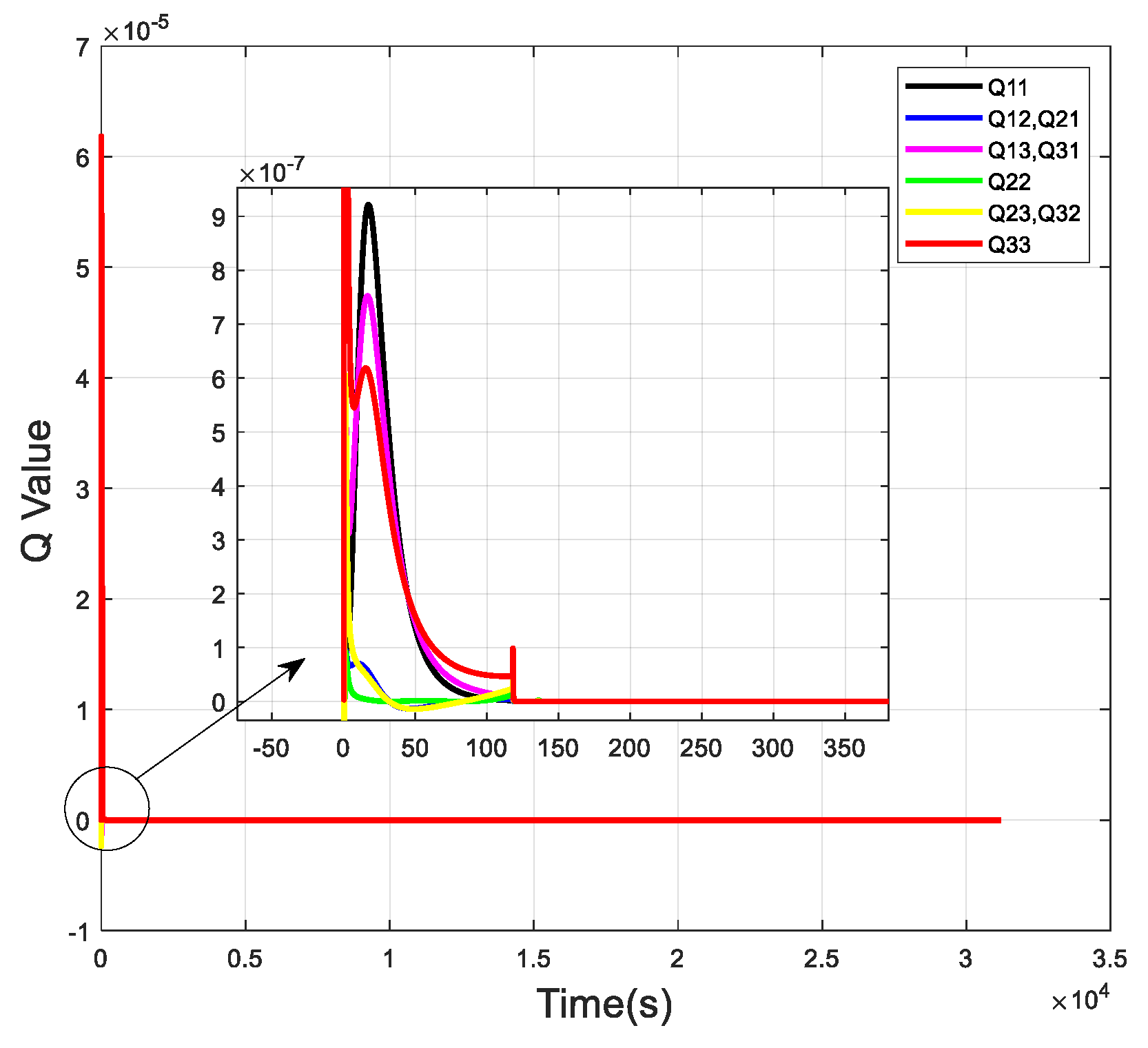
Since the system state variable has a dimension of 3,
is a 3 × 3 symmetric matrix. This paper will represent
as
, where
. The
value when using the AUKF algorithm to estimate the SOC in MATLAB is shown in
Figure 12.
It can be seen from
Figure 12 that since the initial value of SOC is uncertain, the system error is relatively large at this time, so the system noise covariance
is relatively large. By calculating the value of innovation
, and then updating
in real time to correct the error covariance
in time, the system noise is corrected in time, and the value of
approaches to zero.
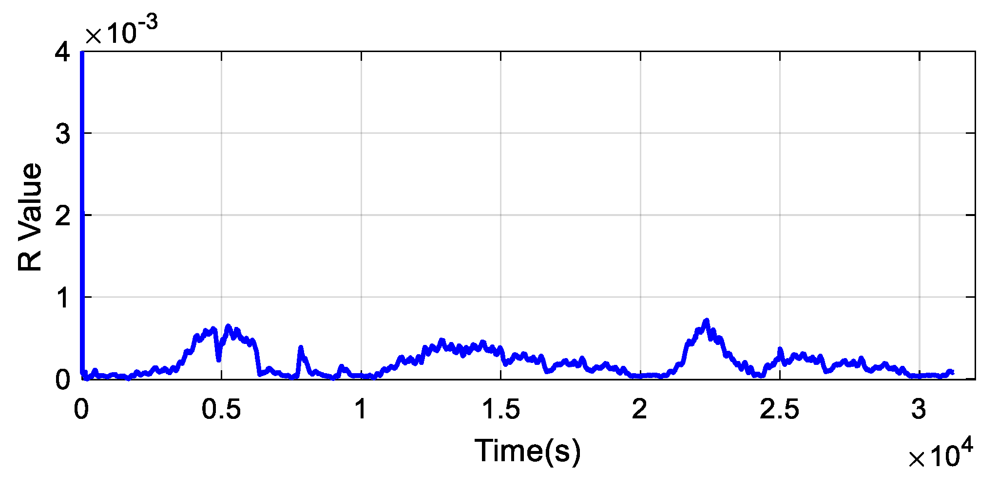
3.2.2. Adaptive Observation Noise Covariance
From Equations (28), (30) and (33), it can be seen that the value of determines the weight of the observation value to the estimated result. When the value increases, the filter gain decreases, resulting in the effect of the observation value on the estimated state value becoming smaller. Conversely, when the value of decreases, the filter gain will increase, which will increase the proportion of the observation value in the estimated state value. Therefore, the observation noise covariance adjusts the Kalman gain in real time to change the proportion of the predicted observation value in the estimation result, thereby reducing the influence of the observation noise on the estimation result.
The residual
at time
is defined as the difference between the actual observation value
and the estimated observation value
. The expression of the residual is shown in Equation (40):
According to the moving window method, the variance of residual
is calculated as:
Through the residual variance
, the observation noise covariance
can be calculated [
37] as shown in Equation (42),
The
value when using the AUKF algorithm to estimate the SOC in MATLAB is shown in the
Figure 13.
It can be seen from
Figure 13 that the value of
fluctuates in a small range. The residual
calculates the difference between the actual observation value and the estimated observation value, and then realizes the real-time update of
, and then adjusts the Kalman gain
to achieve the optimal estimation.
4. Comparison of SOC Estimation Algorithms
The battery SOC was estimated using the unscented Kalman filter algorithm;
and
in the adaptive unscented Kalman filter algorithm were analyzed and simulated—see
Section 3. In this section, we describe how the AUKF algorithm was used to estimate the battery SOC under different load cycles and different initial SOC values. The results of SOC estimation using AUKF algorithm and the results of SOC estimation using UKF algorithm are compared and analyzed.
4.1. Under Pulsed Discharge Conditions
We carried on the simulation experiment in MATLAB, using the AUKF algorithm to carry on the SOC estimation experiment under the pulsed discharge condition. Firstly, the initial values of the AUKF algorithm were set as follows: , , . Then, the AUKF algorithm was used to estimate the SOC under pulsed discharge conditions. The robustness of the proposed AUKF algorithm was tested under different initial SOC conditions. Finally, the results of SOC estimation using UKF algorithm and AUKF algorithm were compared and analyzed.
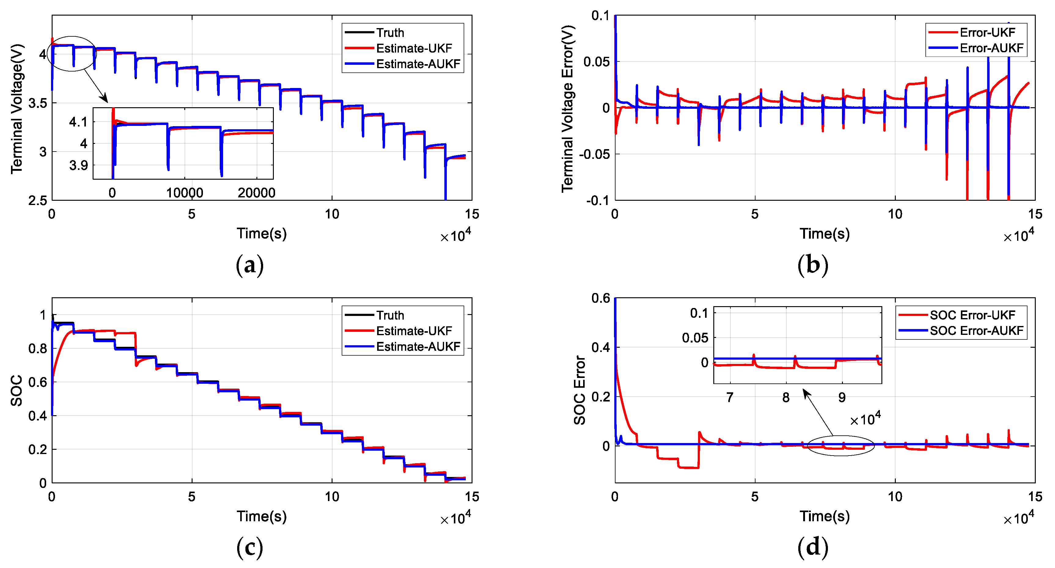
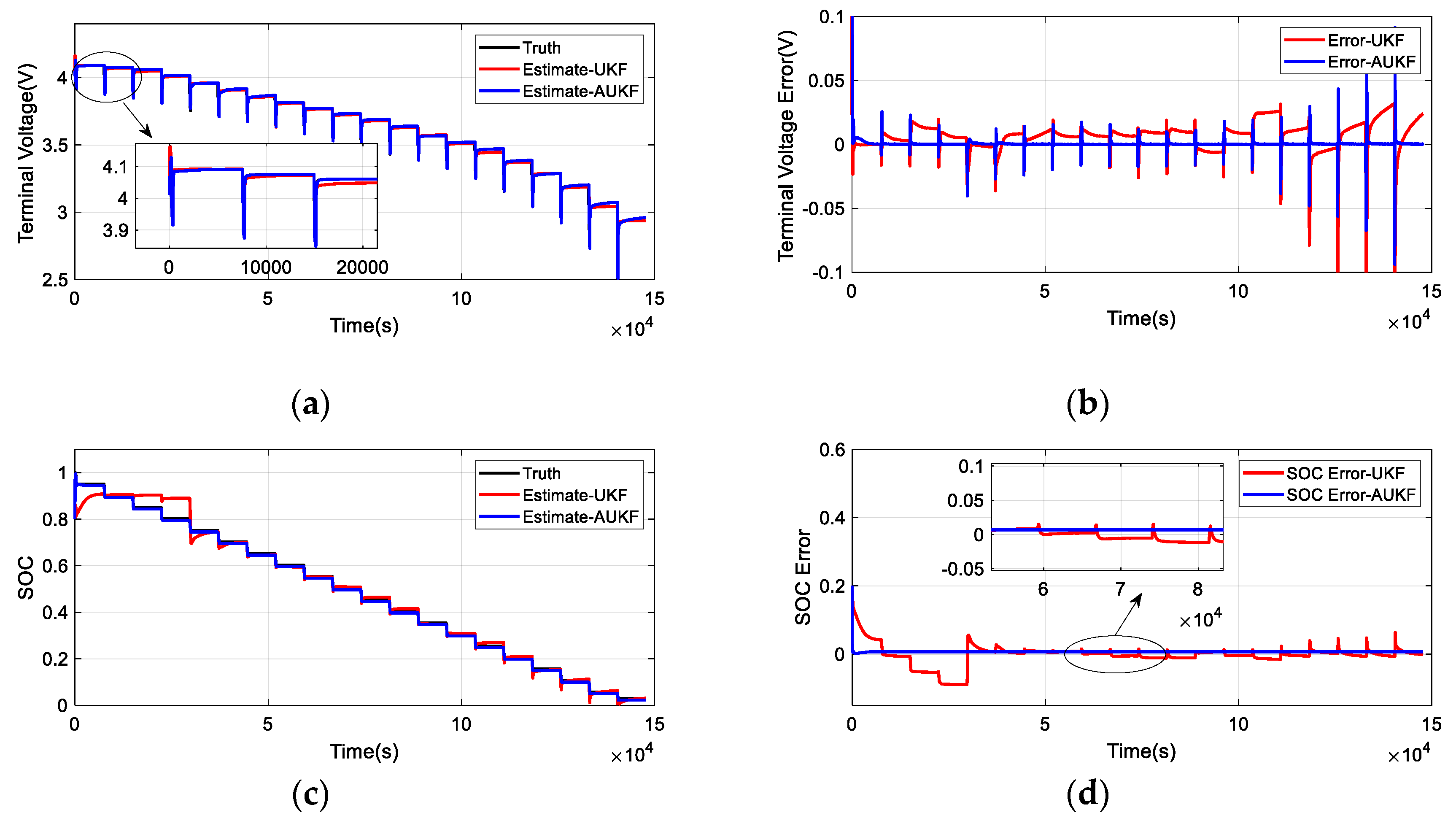
Experiments and analyses were performed under pulsed discharge conditions. For the initial SOC = 0.4, the comparison between the results estimated using the UKF algorithm and the AUKF algorithm is shown in
Figure 14. For the initial SOC = 0.6, the comparison between the results estimated using the UKF algorithm and the AUKF algorithm is shown in
Figure 15. For the initial SOC = 0.8, the comparison of the results estimated using the UKF algorithm and the AUKF algorithm is shown in
Figure 16.
From
Figure 14a,
Figure 15a and
Figure 16a, it can be seen that under pulsed discharge conditions, the value of the battery terminal voltage estimated by the AUKF algorithm is closer to the true value than the value estimated by the UKF algorithm value. From
Figure 14b,
Figure 15b and
Figure 16b, it can be seen that under pulsed discharge conditions, the terminal voltage error value estimated by the AUKF algorithm is smaller than the terminal voltage error value estimated by the UKF algorithm. Additionally, the error value of the terminal voltage estimated by the AUKF algorithm is relatively small. According to
Figure 14c,
Figure 15c and
Figure 16c, it can be seen that the SOC value estimated using the AUKF algorithm is closer to the true value. From
Figure 14d,
Figure 15d and
Figure 16d, it can be seen that the SOC estimation error of AUKF is smaller than that of UKF, and the convergence speed of AUKF algorithm is faster. In summary, under pulsed discharge conditions and different initial SOC conditions, the robustness of the AUKF algorithm for estimating the SOC of the battery is better than that of the UKF algorithm.
4.2. Under UDDS Discharge Conditions
We carried on the simulation experiment in MATLAB, using AUKF algorithm to carry on the SOC estimation experiment under the UDDS discharge condition. Firstly, the initial values of the AUKF algorithm were set as follows: , , . Then, the AUKF algorithm was used to estimate the SOC under UDDS discharge conditions. The robustness of the proposed AUKF algorithm was tested under different initial SOC conditions. Finally, the results of SOC estimation using UKF algorithm and AUKF algorithm were compared and analyzed.
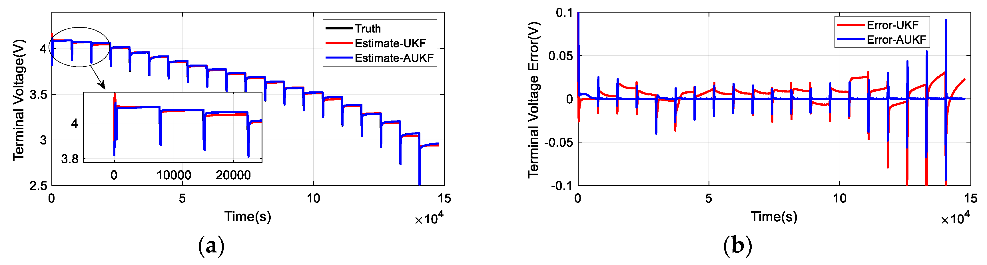
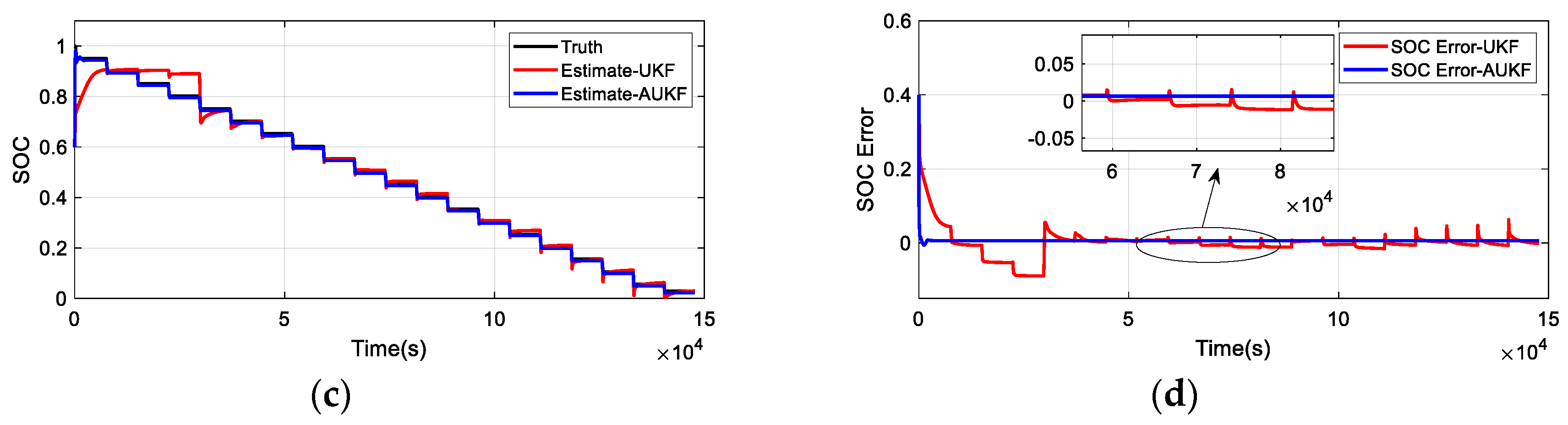
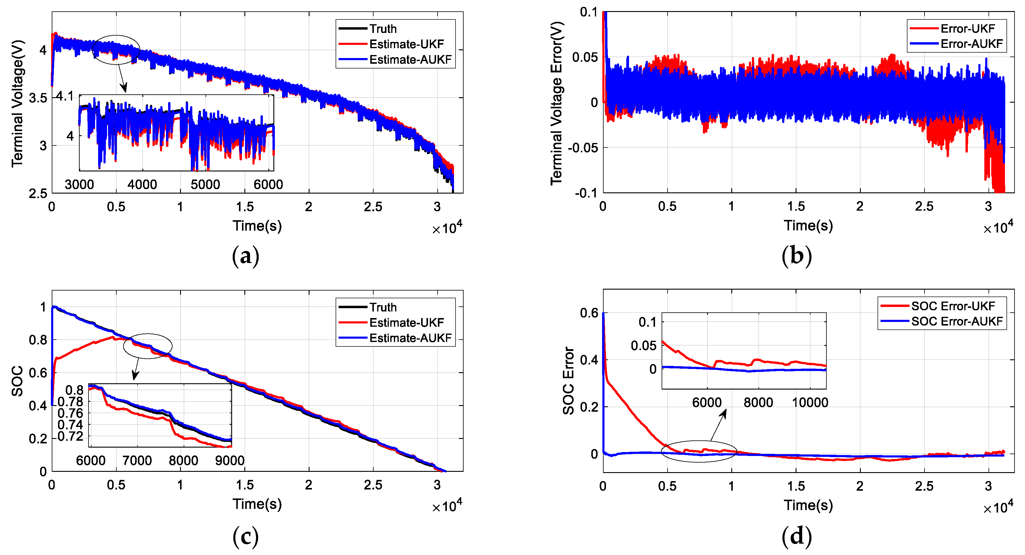
Experiments and analyses were performed under UDDS discharge conditions. For the initial SOC = 0.4, the comparison between the results estimated using the UKF algorithm and the AUKF algorithm is shown in
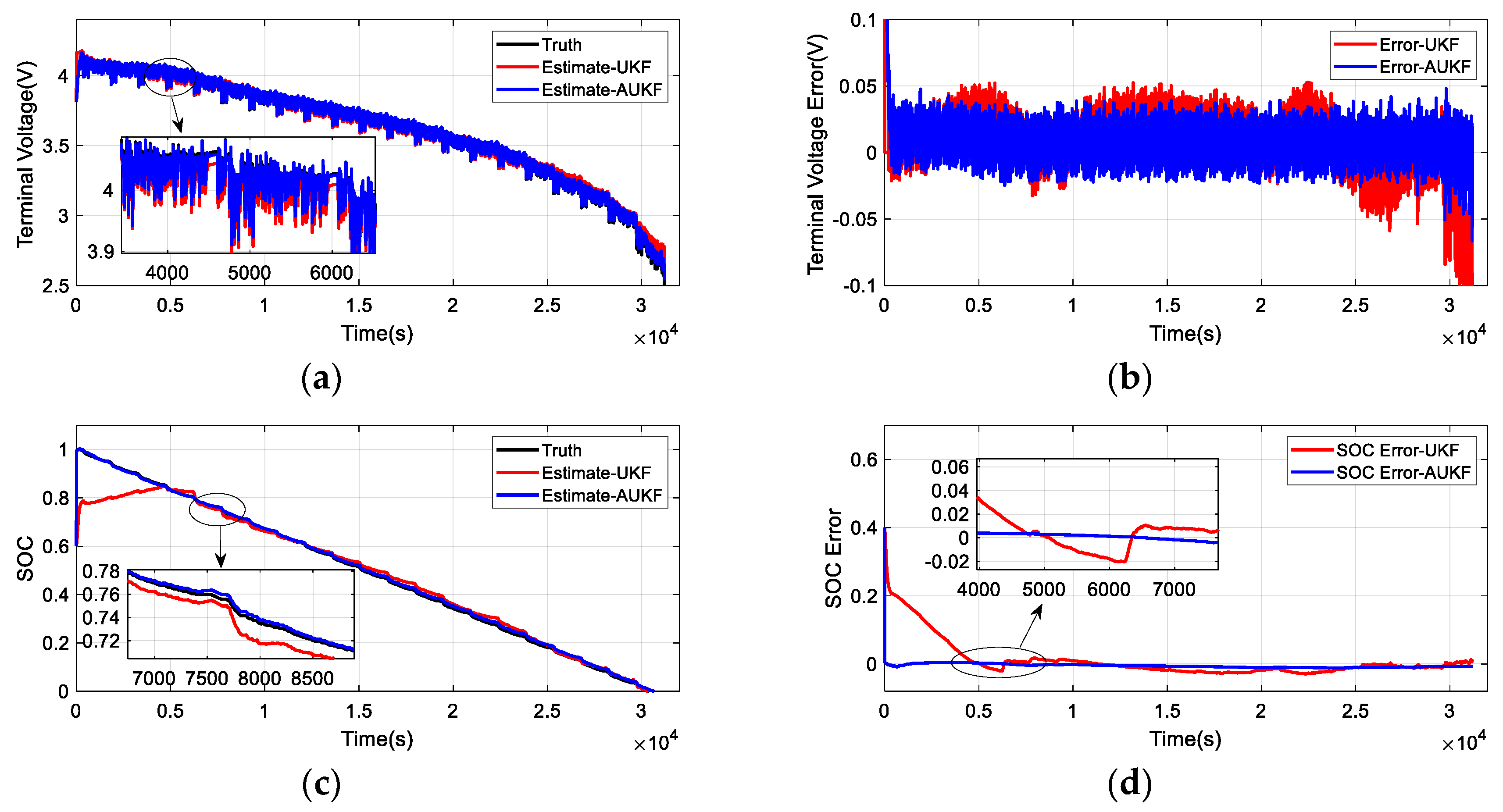
Figure 17. For the initial SOC = 0.6, the comparison between the results estimated using the UKF algorithm and the AUKF algorithm is shown in
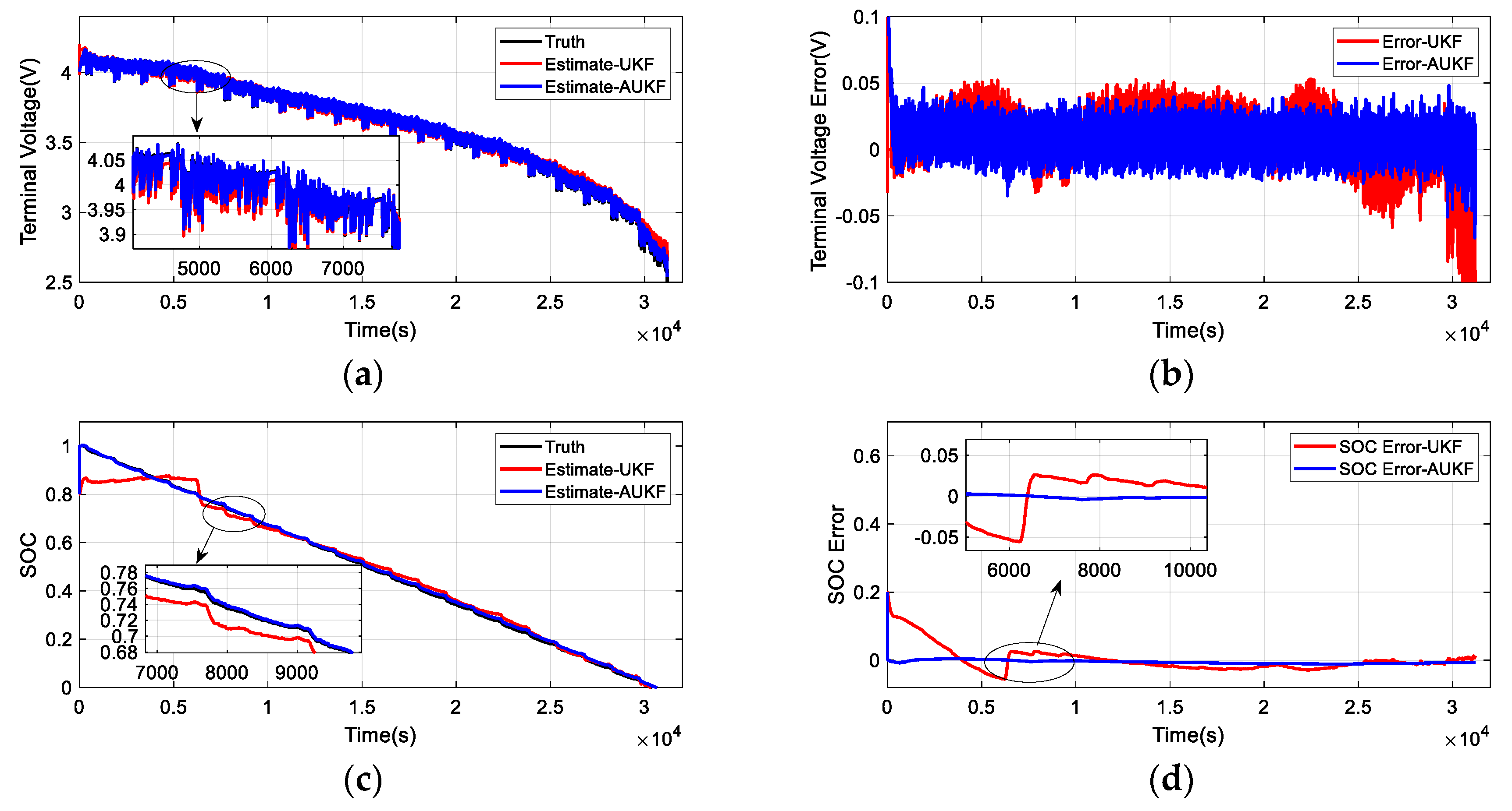
Figure 18. For the initial SOC = 0.8, the comparison of the results estimated using the UKF algorithm and the AUKF algorithm is shown in
Figure 19.
From
Figure 17a,
Figure 18a and
Figure 19a, it can be seen that under UDDS discharge conditions, the value of the battery terminal voltage estimated by the AUKF algorithm is closer to the true value than the value estimated by the UKF algorithm. From
Figure 17b,
Figure 18b and
Figure 19b, it can be seen that under UDDS discharge conditions, the terminal voltage error value estimated by the AUKF algorithm is smaller than the terminal voltage error value estimated by the UKF algorithm. Additionally, the error value of the terminal voltage estimated by the AUKF algorithm is relatively stable. According to
Figure 17c,
Figure 18c and
Figure 19c, it can be concluded that the SOC value estimated using the AUKF algorithm is closer to the true value. From
Figure 17d,
Figure 18d and
Figure 19d, it can be seen that the SOC estimation error of AUKF is smaller than that of UKF, and the convergence speed of AUKF algorithm is faster. In summary, under UDDS discharge conditions and under different initial SOC conditions, the robustness of the AUKF algorithm for estimating the SOC of the battery is better than the UKF algorithm.
In order to further verify the accuracy of the SOC estimation by the AUKF algorithm, the terminal voltage value and the SOC value estimated by the UKF algorithm and the AUKF algorithm were subjected to error analysis. The error results of the battery SOC estimation under different load cycles and different initial SOC values were averaged. The error analysis results of the terminal voltage are shown in
Table 5. The error analysis results of the estimated SOC are shown in
Table 6.
The mean absolute error (MAE) can avoid the problem of the deviations cancelling each other out, and can well describe the degree of data dispersion. The root mean square error (RMSE) measures the deviation between the observation value and the true value, and can well reflect the accuracy of the measurement.
Table 5 shows that the MAE of the terminal voltage estimated by AUKF was smaller, indicating that the terminal voltage estimated by AUKF is less discrete than that of UKF algorithm; the RMSE of terminal voltage estimated by AUKF algorithm was smaller than that of UKF algorithm.
Table 6 shows that the SOC value estimated by the AUKF algorithm had a smaller MAE than that of UKF algorithm. The RMSE of SOC estimated by AUKF algorithm was 2.6% smaller than that of UKF algorithm. The above error analysis results indicate that the accuracy of SOC estimation using AUKF algorithm is better than that of UKF algorithm.


