1. Introduction
Owing to growing interest in industrial robots, various robots have been utilized in manufacturing sites. Previously, in the teaching process, skilled operators manually moved a robot and recorded its position in the robot controller. The recorded position was then replayed by performing a point-to-point or continuous-path motion in a real robot [
1,
2,
3]. Using this teaching process, the robot can execute pick and place, loading and unloading, and assembly tasks in the manufacturing site. However, for the same robot to adapt to more complex and flexible tasks such as painting, polishing, welding, etc., the complicated and optimal paths or trajectory planning methods are required [
4,
5,
6,
7,
8,
9]. One of the core processes in a shoe manufacturing factory [
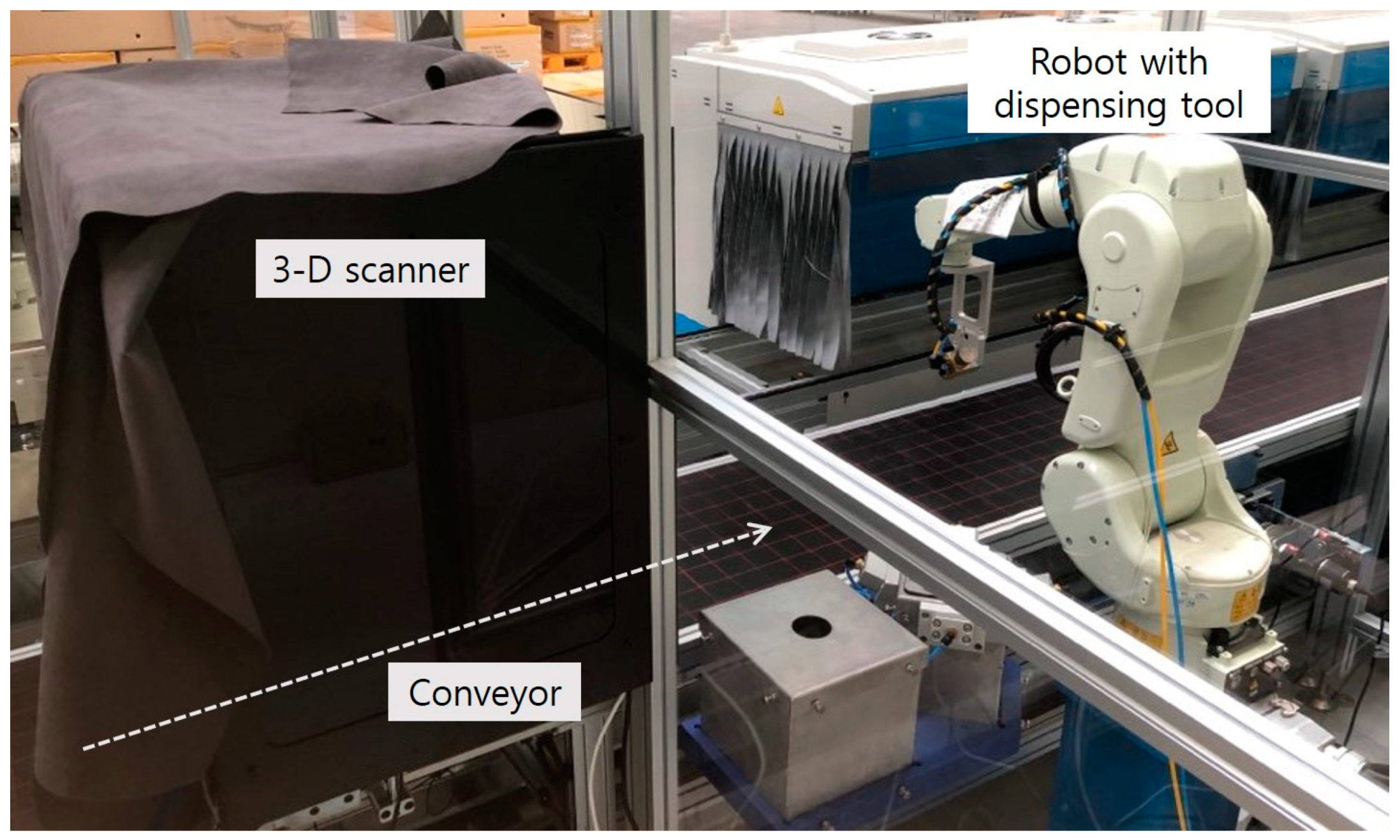
10] is attaching a sole to the upper part of a shoe, after applying adhesive to the upper contour of the sole. If a robot is adapted to this gluing task, its Tool Center Point (TCP) should follow the 3-D contour path of the sole with a uniform dispensation of the glue. For the robot to move through this contour, a trajectory should be planned a priori. This trajectory is planned by connecting intermediate points on the contour obtained from the CAD data of the sole or from the point cloud scanned in the 3-D scanner while the target object is being moved by a conveyor, as shown in
Figure 1.
If the robot moves several consecutive points without stopping at each point, a smooth spline path is required to avoid discontinuity of velocity. The points through which the robot passes are called knots or knot points. This spline method has been widely applied to create paths for many systems such as mobile robots [
11], vehicles [
12], unmanned aerial vehicles (UAVs) [
13], and manipulators [
14,
15]. Actual examples of robotic tasks include welding, dispensing glue, and painting, where a manipulator must move continuously through multiple defined knots in a manufacturing site.
In the motion planning of the robot, path planning is used to find a series of the positions of robot end effectors without collision. However, in trajectory planning, it is necessary to move the real manipulator to determine the position, velocity, and acceleration of the robot over time. Sampling-based motion planning [
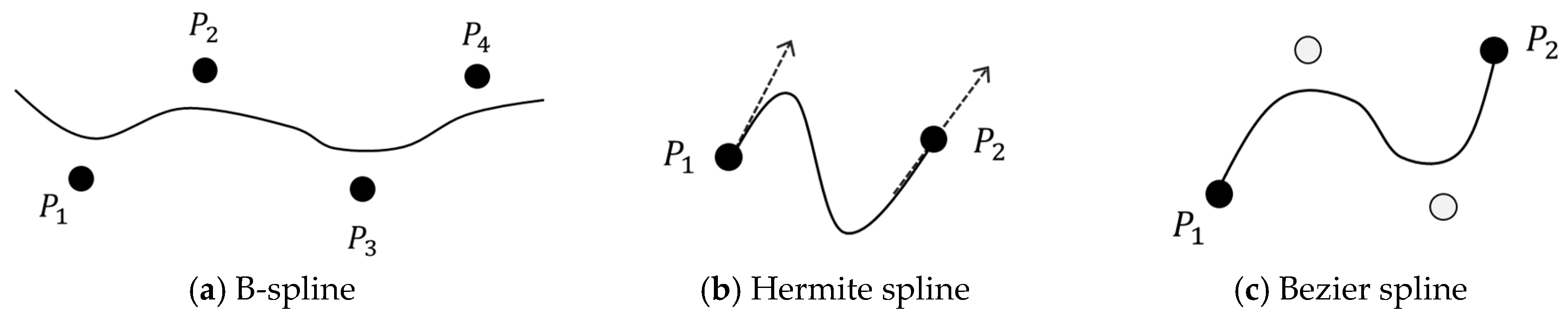
16] is widely used in path planning to find a collision-free path. However, it cannot be used to derive closed-form solutions to plan this trajectory. To apply to industrial robots, closed-form solutions are required to assign a position, velocity, and acceleration to them at each sampling time. Consequently, previous studies used other methods such as B-spline, cubic spline, trigonometric spline, and Bezier spline to plan a trajectory for multi-points [
17,
18,
19,
20,
21,
22,
23,
24,
25,
26]. The spline trajectory planning method can be divided into trajectory planning in the joint space and trajectory planning in the task space (Cartesian coordinate space). In the joint space, the cubic spline method is primarily used to generate the trajectory of each joint such that the change in angle of each joint is connected without stopping during motion. The joint vector at each knot should be calculated using inverse kinematics before applying the trajectory planning method. In the concept of the trajectory planning in the task space, the time series of position in the task space are derived at every sampling time. Then the joint vectors at each sampling time are calculated with inverse kinematics and the robot controller moves joint angles. Basically, the operators intuitively assign and record each knot of the manipulator in the real manufacturing site. Therefore, it is necessary to propose a new method to plan spline trajectory in the task space.
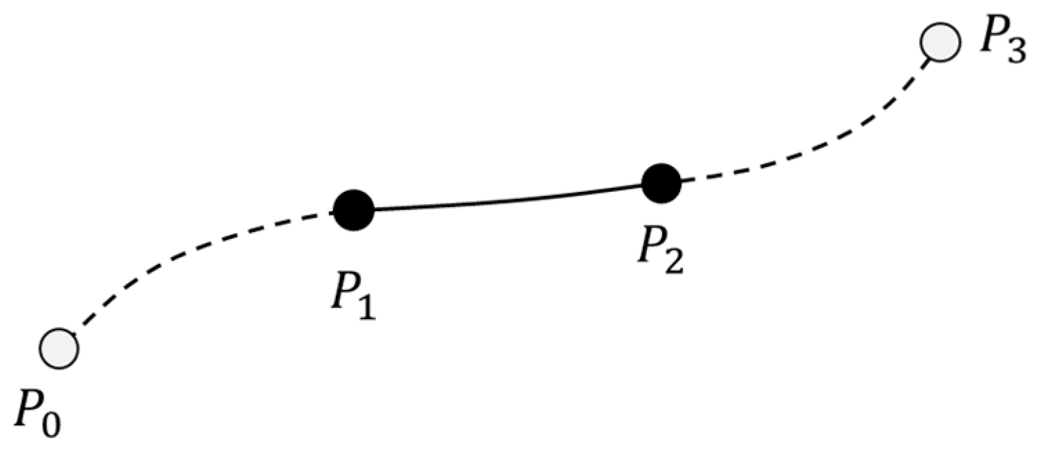
In the task space, the Catmull–Rom spline can be used to plan the spline path [
27] because it is simple and requires little computation. The Catmull–Rom spline is primarily used in computer graphics applications to draw paths that connect multiple points smoothly [
28], in order to satisfy the continuity of velocity at each point [
29]. At these points, Catmull–Rom can be applied to plan the trajectory of the robot manipulator. However, it is necessary to first derive the velocity and acceleration functions for the trajectory planning of the robot. A method is required to assign initial and final velocities while a systematic consideration is necessary to plan the trajectory for complicated industrial applications such as following a closed-loop contour at uniform speed. To apply this to the robot, it is necessary to maximize productivity by minimizing its cycle time [
30]. Previous studies considered this problem and proposed a method for an optimal trajectory using jerk bounding [
31,
32] or by considering velocity and acceleration [
33]. However, determining the jerk limit of a robot is difficult and counterintuitive [
34]. Therefore, it is necessary to optimize the velocity and acceleration of the robot considering limit conditions such as maximum speed and acceleration.
In this study, a simple novel method is proposed to generate a spline trajectory in a task space to allow the robot to move through multiple knots. To help the basic Catmull–Rom spline adapt to the robot trajectory planning problem, the authors propose an iterative segmentation method for multiple knots and present a method that determines control points outside the trajectory, such that the initial and final velocities of the motion are zero. To minimize the operating time of the robot and stay within the physical limit value, an optimization method that considers the physical maximum velocity and acceleration of the robot is presented. The systematic planning process is presented for applications in complicated industrial tasks, to enable the robot to follow the 3-D contour at uniform speed. The proposed methods are evaluated via simulation in various cases and to compare computational load with the cubic spline method. They are also implemented with an experiment that involves dispensing adhesive uniformly to the upper contour of the sole of a shoe at a shoe manufacturing factory. The results show that the proposed trajectory planning in the task space can be applied to the robotic task in actual manufacturing processes.
Section 2 introduces related studies and a basic Catmull–Rom spline in detail. In
Section 3, the method for creating the task space trajectory based on the Catmull–Rom spline is explained with the simulation. An experiment to test the proposed method on real industrial robotic tasks are described in
Section 4. Finally,
Section 5 contains the discussion and conclusion of this study.
3. Trajectory Planning for Multiple Knots
3.1. Iterative Segmentation for Multiple Knots
The Catmull–Rom spline is basically utilized to find paths in order to connect two points. Therefore, the Catmull–Rom spline method should be sequentially applied by connecting two consecutive neighboring points to generate a trajectory via multiple knots.
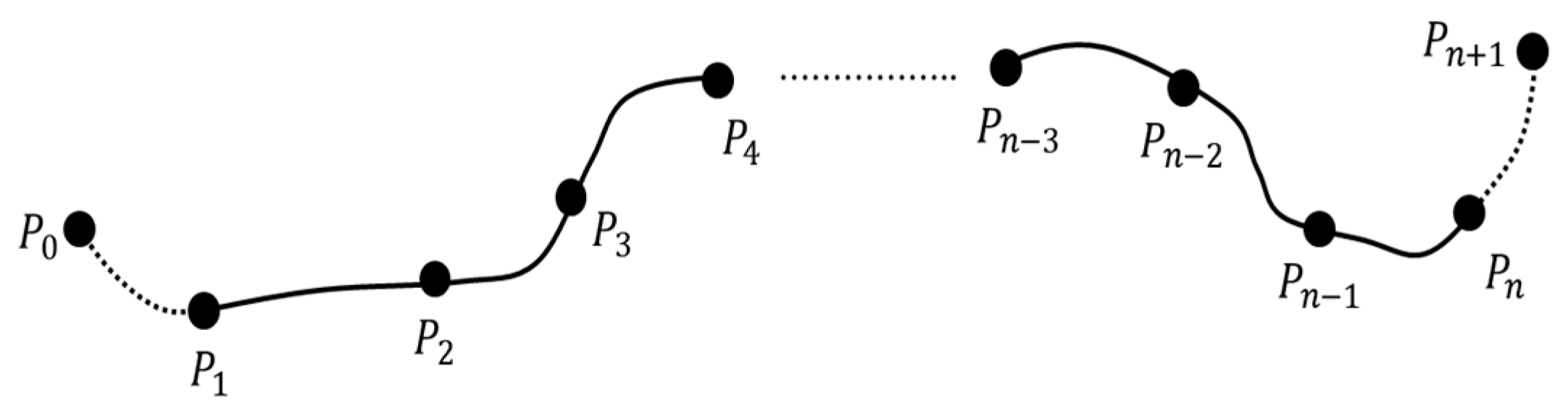
Figure 4 shows an example of
n knots starting at
up to
.
To connect
and
in the first segment, two control points are required. One control point can be designated as the next knot
. For the other control point, a virtual control point
can be selected using the constraint that maintains the velocity at
at zero because
is the starting position in the overall path. From Equation (2), the velocity at
is zero when
is equal to
, as expressed in Equation (8).
To derive the path in the subsequent segment, two control points are placed using the points that immediately precede and follow them. When the last segment connects to , similar to the first segment, the virtual control point can be replaced with , such that the velocity at becomes zero in Equation (9). Therefore, the first control point and last control point of the entire trajectory can be determined. Equations (5)–(7) can be applied repeatedly to obtain the position, velocity, and acceleration of the entire trajectory.
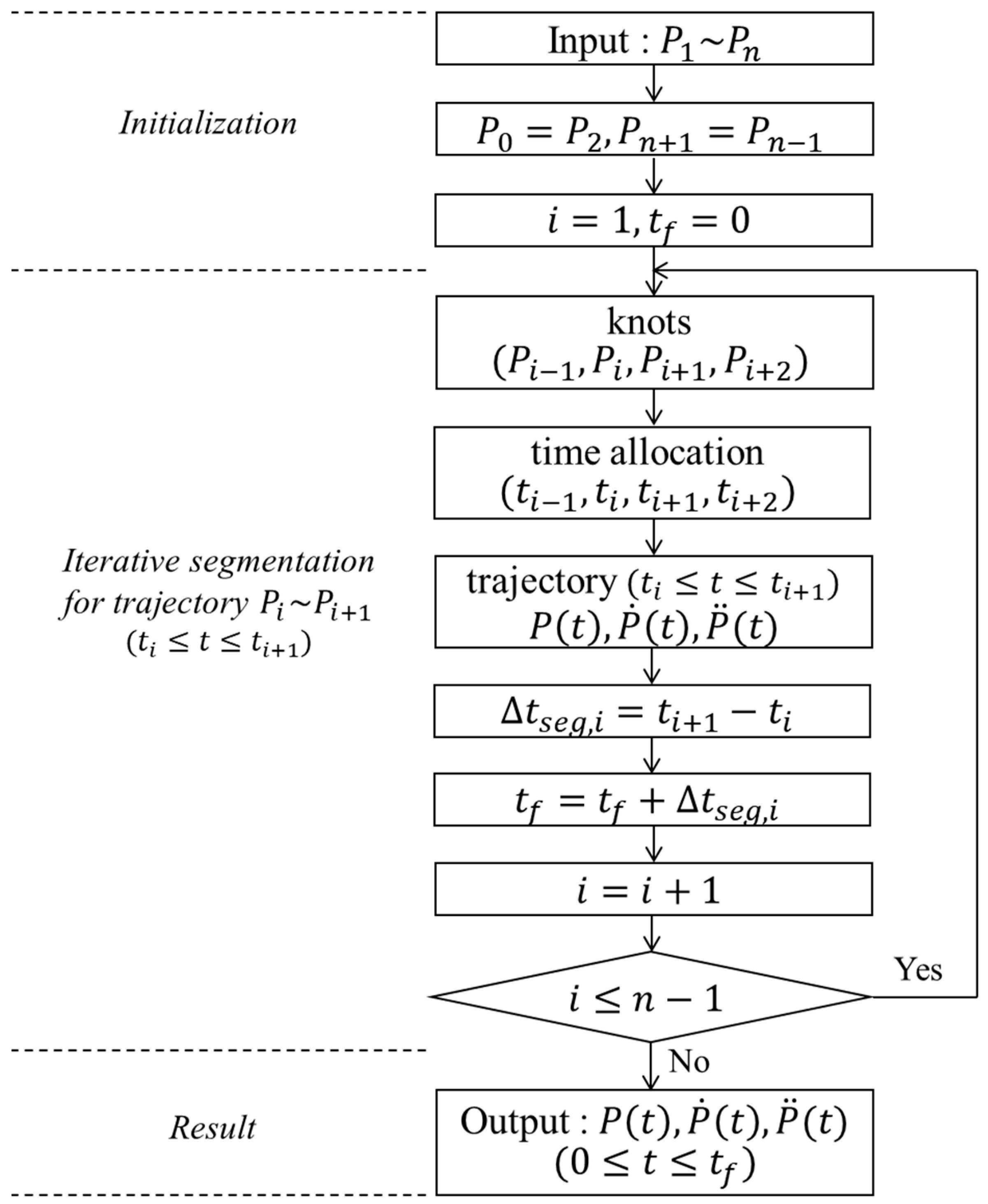
The process to plan trajectory from
to
is represented as a flowchart in
Figure 5. Two virtual control points,
and
, are assigned using (8) and (9) when the
n multiple knots are given. Every four knots are selected as a segment from
to
, and trajectory from
to
are iteratively calculated using Equations (4)–(7). Then position, velocity, and acceleration for the entire path can be derived as a result and final motion time can be found as
. Simulation to evaluate the proposed method is performed with MATLAB in the computer operated by Windows operating system. The source code for the algorithm is implemented as a script language in MATLAB without using a toolbox.
The simulations used to move multiple knots in the task space are executed using data in
Table 1. The first simulation is implemented to show trajectory planning when all segments have an equal distance with knots in the task #1. In the second simulation, each segment has a different distance as knots in the task #2.
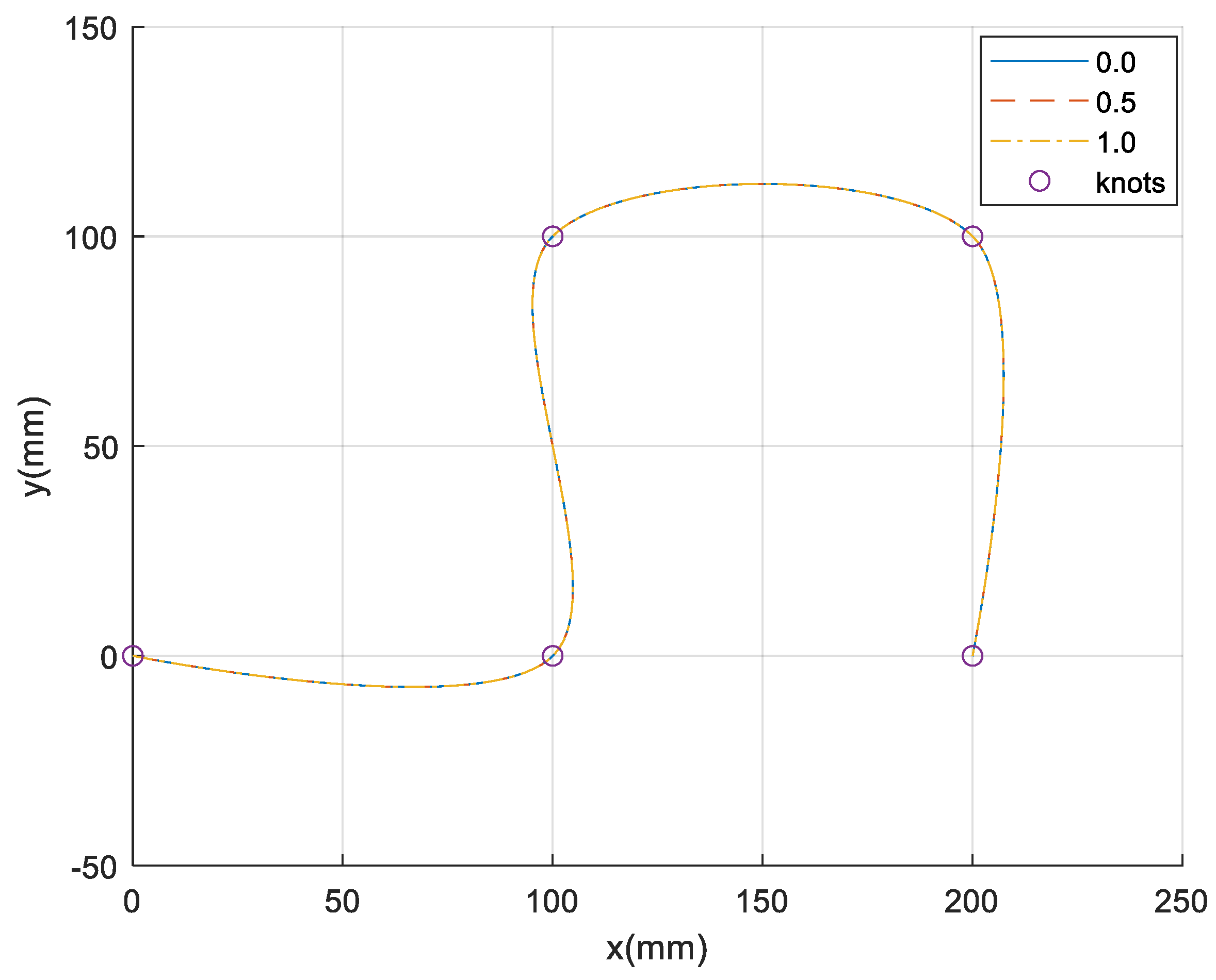
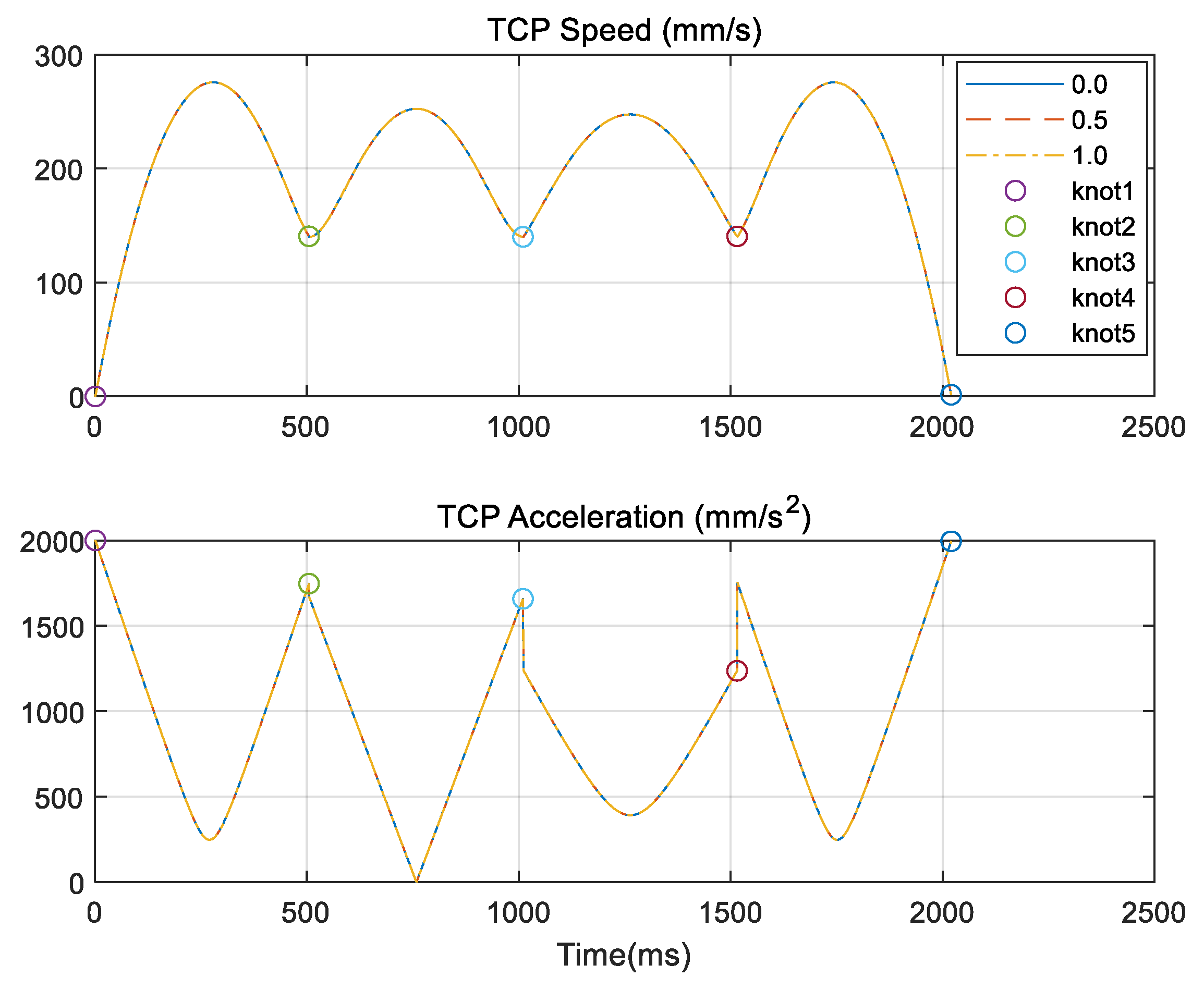
The target path in the task #1 consists of five points, and the distance between two points in each segment is 100 mm. The result of the planned path using the proposed method is shown in
Figure 6. The given knots are represented as a circle at each point, and each line corresponds to the case when
in Equation (3) is changed from 0 to 1. The velocity and acceleration of the TCP of the robot are shown in
Figure 7. The results show that the three trajectories are exactly the same even when a different
is applied. The velocity at the initial or final point is zero, and the trajectory exhibits continuity in velocity at each point. This shows that the trajectory remains consistent regardless of the value of
, provided all segments are uniform in length.
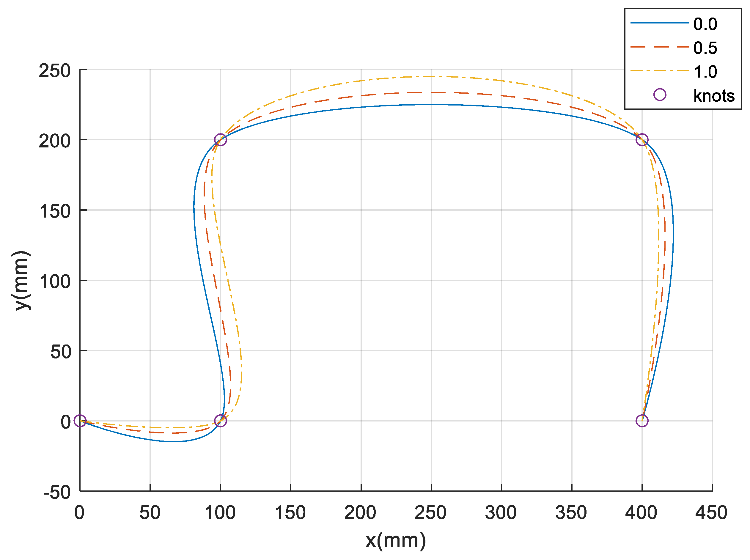
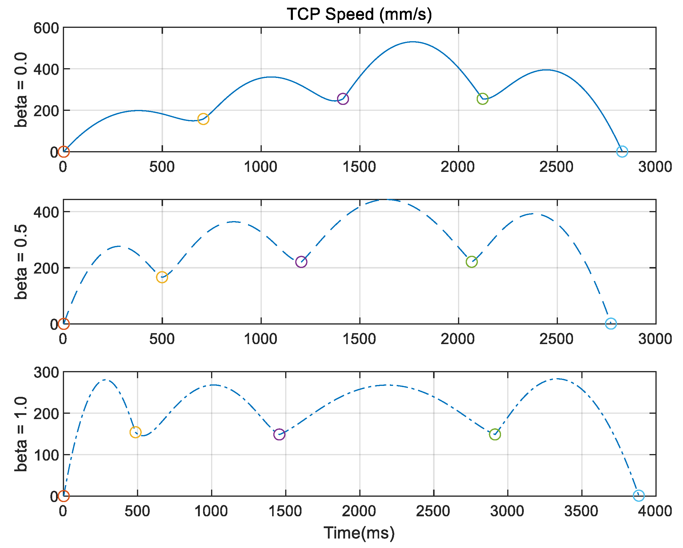
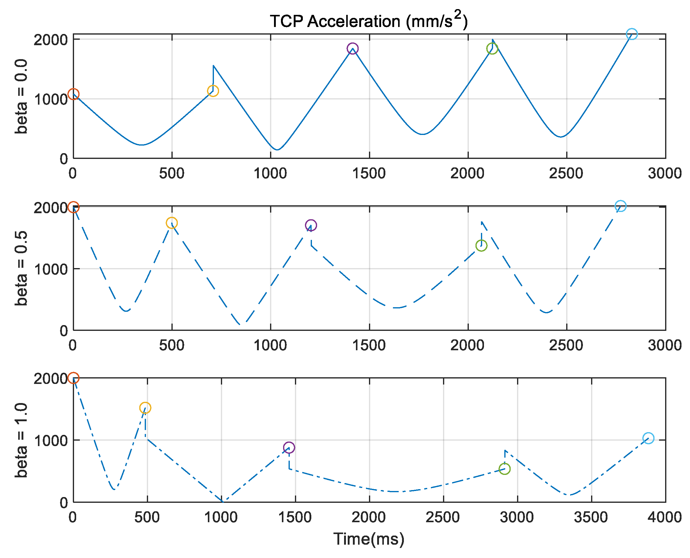
In the second simulation with the task #2, each segment has its own distance, from 100 mm to 300 mm. The result of the planned path is shown in
Figure 8 and its velocity and acceleration profiles are represented in
Figure 9 and
Figure 10, respectively. As shown in these figures, the path and trajectory change according to the value of
. As shown in the third segment with the longest distance between points 3 and 4, a long motion time is required and this motion follows the long path in the chordal case (
). This occurs because the time in each segment is proportional to the relative distance between two points. However, the deviation in the velocity at each segment is relatively small when
is one. Therefore, if the robot is required to move at a relatively uniform speed to execute the spline motion,
can be chosen as one.
3.2. Comparison with Cubic Spline
The proposed method based on the Catmull–Rom spline is compared with the previous spline method used in the interpolation. The representative method is the planning using a cubic spline curve. It has a piecewise-cubic trajectory, which passes through the multiple waypoints and satisfies velocity continuity at each waypoint. The simulation is implemented using knots in the task #1 and the task #2 to show computational efficiency and shape of the curve.
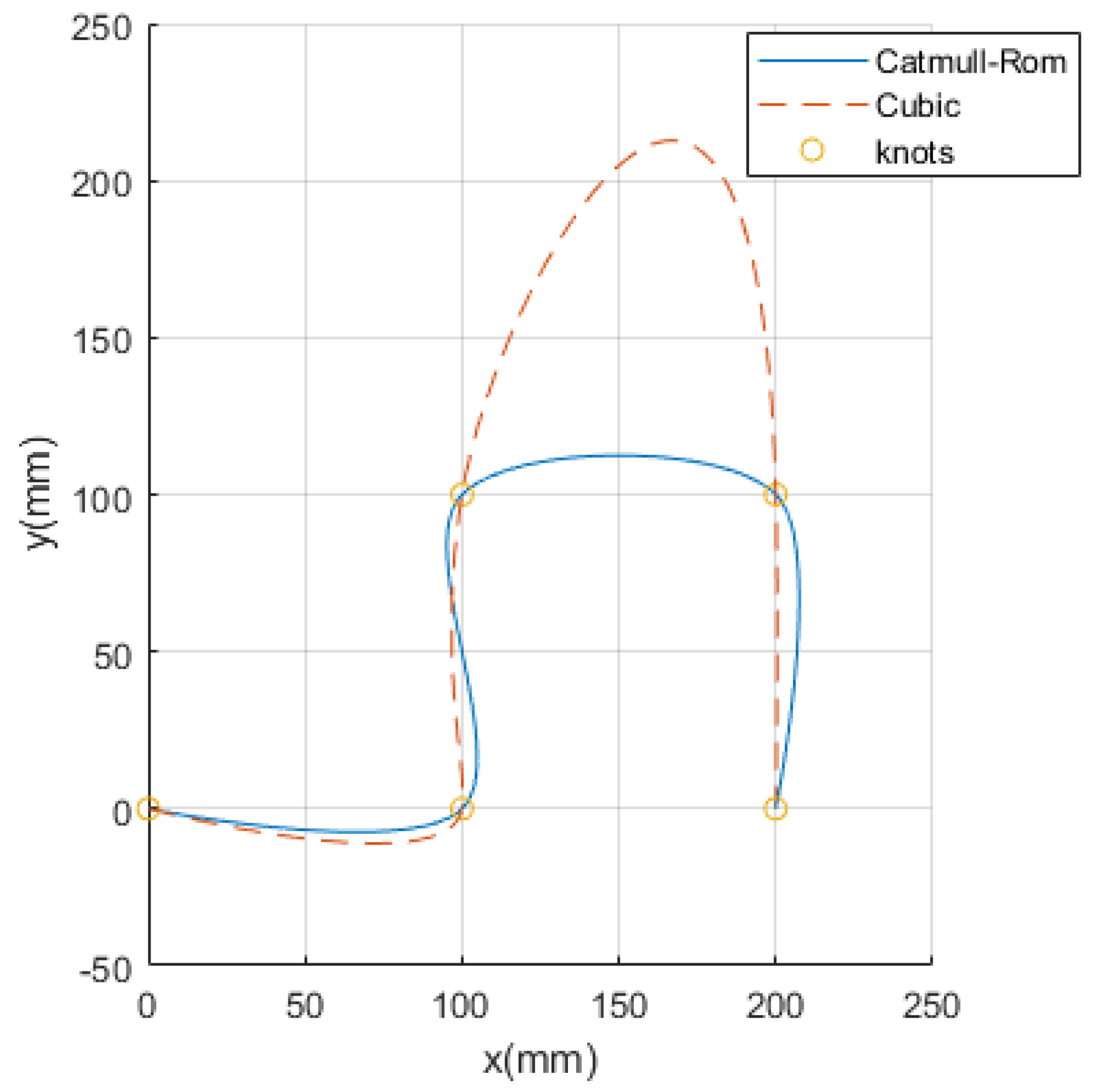
In
Figure 11 and
Figure 12, the difference between the two results can be shown. The paths are compared in
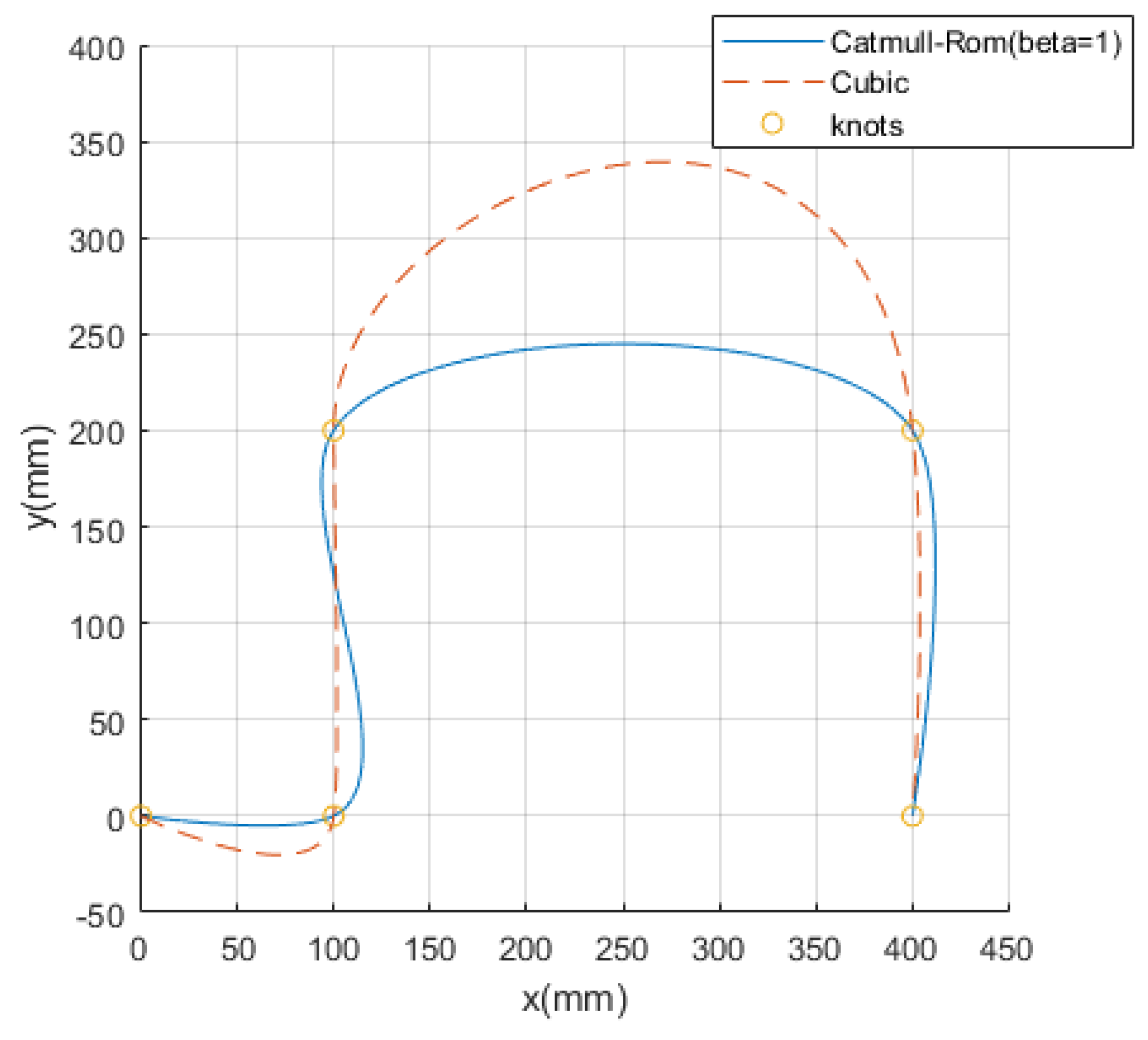
Figure 11 when knots in the task #1 are used for planning. A large overshoot exists between the third and fourth waypoints when the cubic spline is applied.
Figure 12 shows the paths from knots in the task #2 and a large overshoot can be shown in the same segment. It means that the curve using cubic spline can exert large overshoot as mentioned in reference [
24].
The computation time is measured while these simulations are executed to compare computational efficiency for two methods. This simulation is performed with MATLAB in the computer operated by Windows 10. It has an Intel Core i7 4 GHz CPU with 32 GB RAM. The 20 simulations are performed, and the average time and standard deviation are listed in
Table 2. The results show that it takes less time in about 5.7~5.8 ms when the Catmull–Rom is used compared with cubic spline. Therefore, it can be concluded that the proposed method requires less computation.
3.3. Optimization of Velocity and Acceleration
Because the trajectory generated by the iterative segmentation procedure is determined by the time passed by each point in Equation (4), the physical maximum velocity and acceleration of the actual robot are not considered in the magnitudes of the velocity and acceleration. To minimize the operating time of the robot and maintain its physical limit value, it is important that velocity and acceleration would cause the trajectory to move lower and closer to the maximum velocity and acceleration to which the robot can move.
The points where the velocity and acceleration of the robot are maximum in the trajectory are those points where the derivatives of its position and velocity are zero. The time corresponding to the trajectory of the actual robot movement in one segment is between and . The maximum velocity and acceleration in each segment can be estimated from Equations (6) and (7). When these values are determined in the entire segments, the maximum velocity and maximum acceleration can be predicted in the entire trajectory.
To optimize the velocity and acceleration of motion and enable the robot to follow the planned trajectory, the maximum velocity
and the maximum acceleration
in the task space of the real robot should be determined. If the initial and final velocities in the trajectory are zero, the maximum velocity and maximum acceleration of the robot can be changed according to the ratio of the motion time. The parameters
and
representing this ratio can be calculated using Equation (10) because the velocity is linear with time and acceleration is proportional to the square of time. By determining the maximum ratio value
in Equation (11) and multiplying it by the motion time
, the optimized motion time
can be obtained, as expressed by Equation (12). Hence, by redistributing the motion time according to this ratio, the actual velocity and acceleration of the robot can be approximated to the physical maximum value, and the motion of the robot can be optimized.
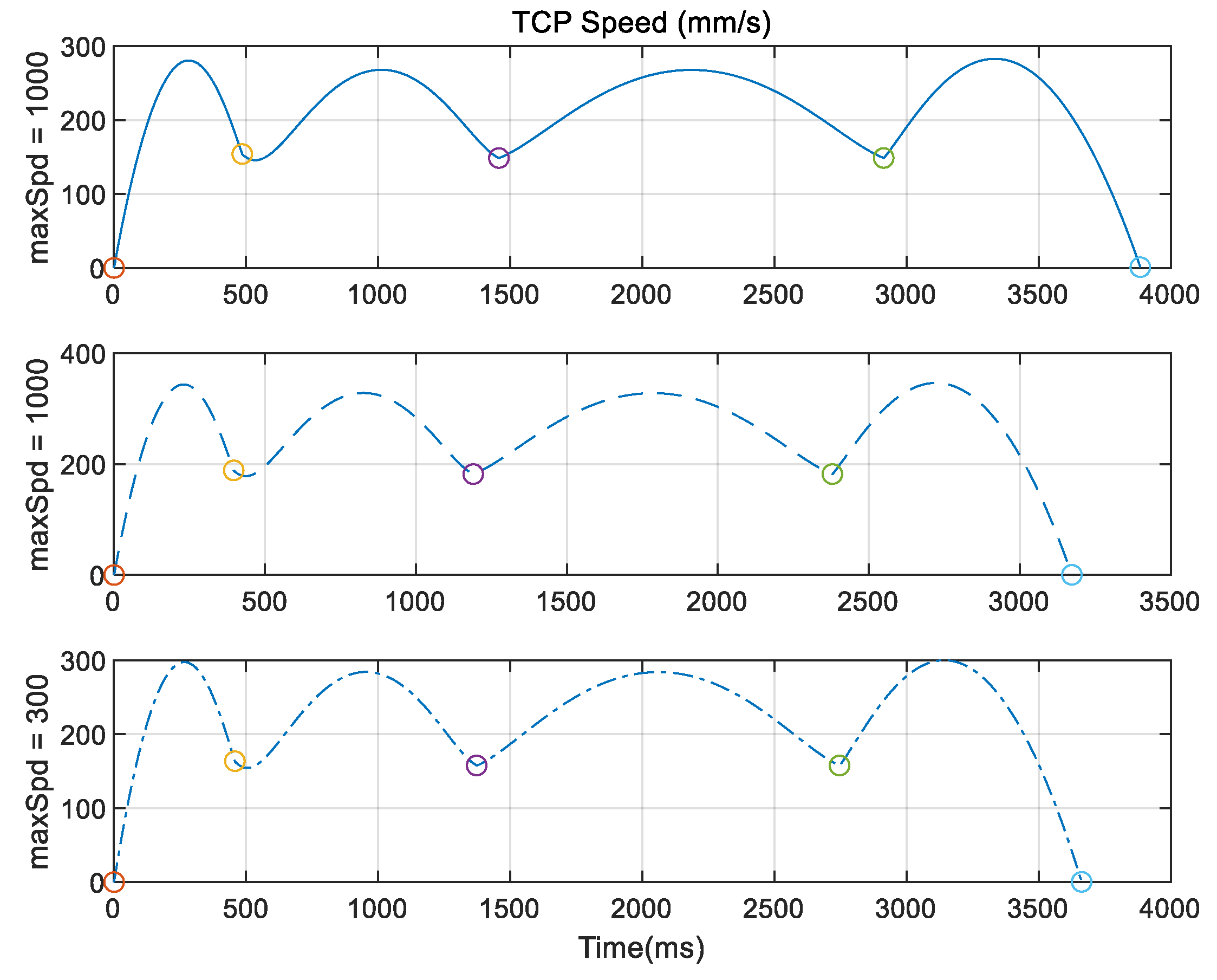
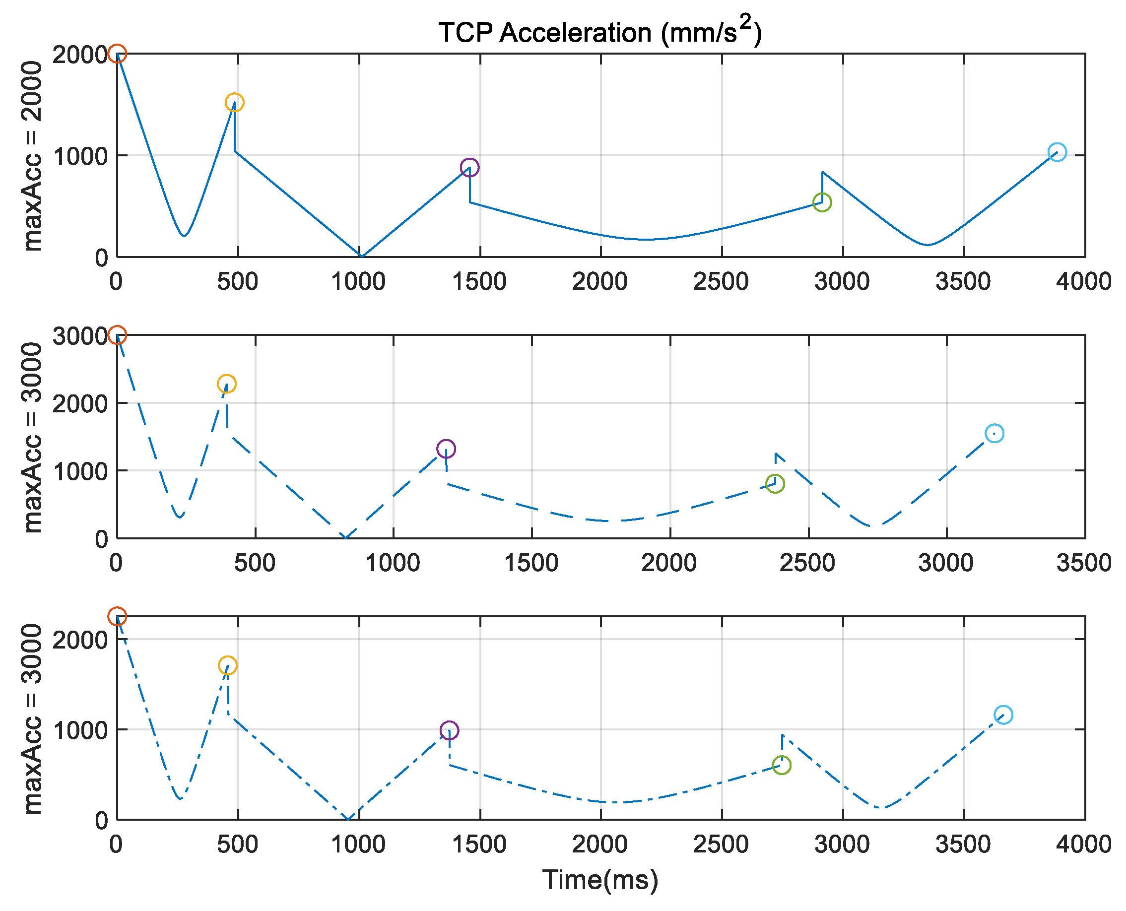
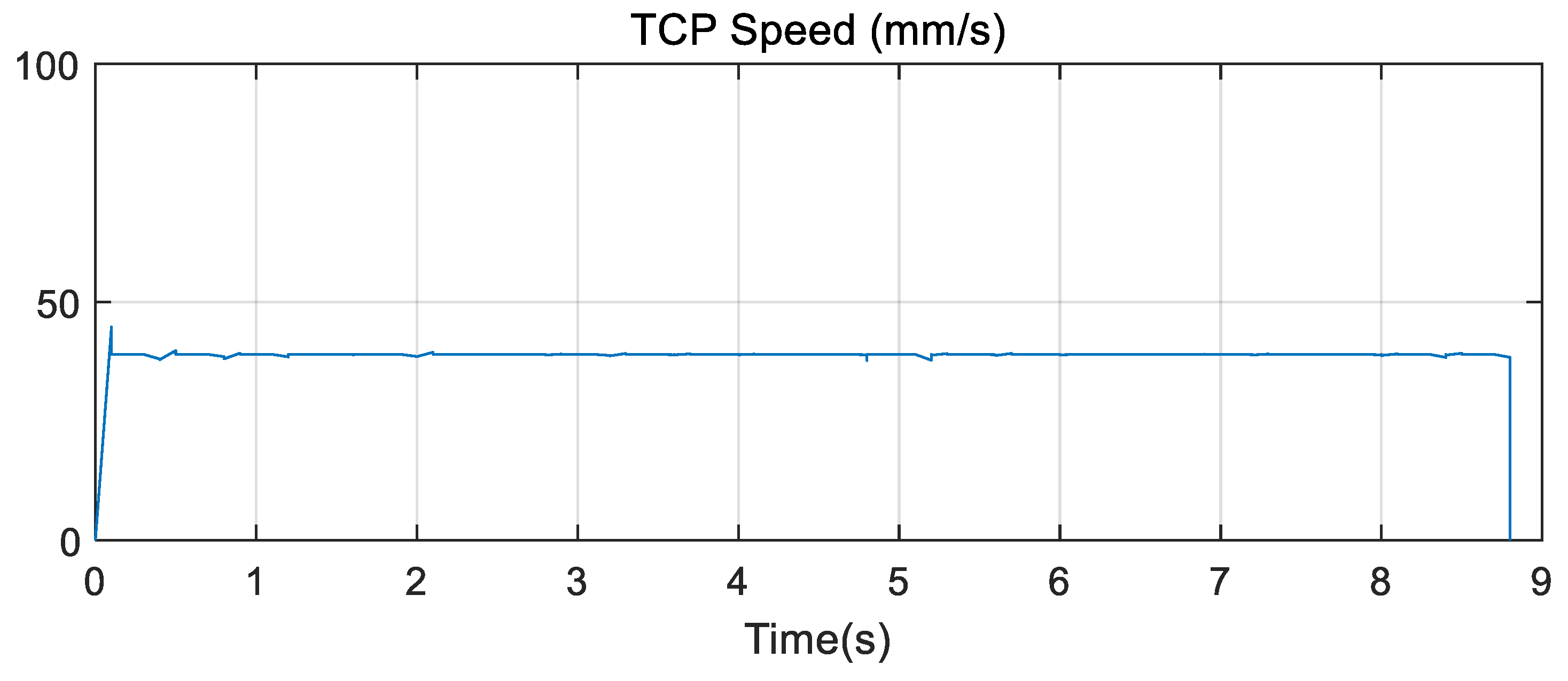
The effect of optimizing the time of motion is evaluated in the simulation with task #2. To evaluate the optimization of the motion time, three cases are compared with the knots in task #2 and
is set to 0, as shown in
Table 3. The resulting velocity and acceleration are shown in
Figure 13 and
Figure 14, respectively. In the first case, the maximum velocity is less than 300
. However, the maximum acceleration is 2000
when time is zero and is equal to
. The
is then changed to 3000
in the second case. Subsequently, the maximum acceleration in the planned trajectory becomes 3000
and motion time is decreased by approximately 0.7 s. This means that motion is optimized by satisfying the acceleration limit. In the third case,
is set at 300
to verify the effect of the velocity limit. The third plot in
Figure 13 shows that the maximum velocity in the trajectory is equal to
, whereas maximum acceleration is less than
, as shown in the third plot in
Figure 14. This shows that motion is optimized by limiting the maximum velocity of the robot.
5. Conclusions
In this study, the authors proposed a method for generating the trajectory of a robot using the spline method, which allows the robot to move several points without stopping in a task space. The basic interpolation was based on the Catmull–Rom spline, which satisfied the continuity of velocity at each knot. To adapt a basic Catmull–Rom spline to the robot trajectory planning problem, a method was proposed to select control points outside the trajectory such that the initial and final velocities of the robot were zero. The simulation results demonstrated that the trajectory did not change with respect to time at each knot when the relative distance between two neighboring points was constant for the entire path. However, when the relative distance was varied and the chordal Catmull–Rom spline applied, the robot moved at a relatively uniform speed to execute a spline motion, in which the time in each segment was determined to be proportional to the relative distance between two points.
By proposing the motion time redistribution method based on the maximum velocity and acceleration of the robot, the motion time of the actual robot could be optimized. This was verified via simulations using various maximum velocities and accelerations.
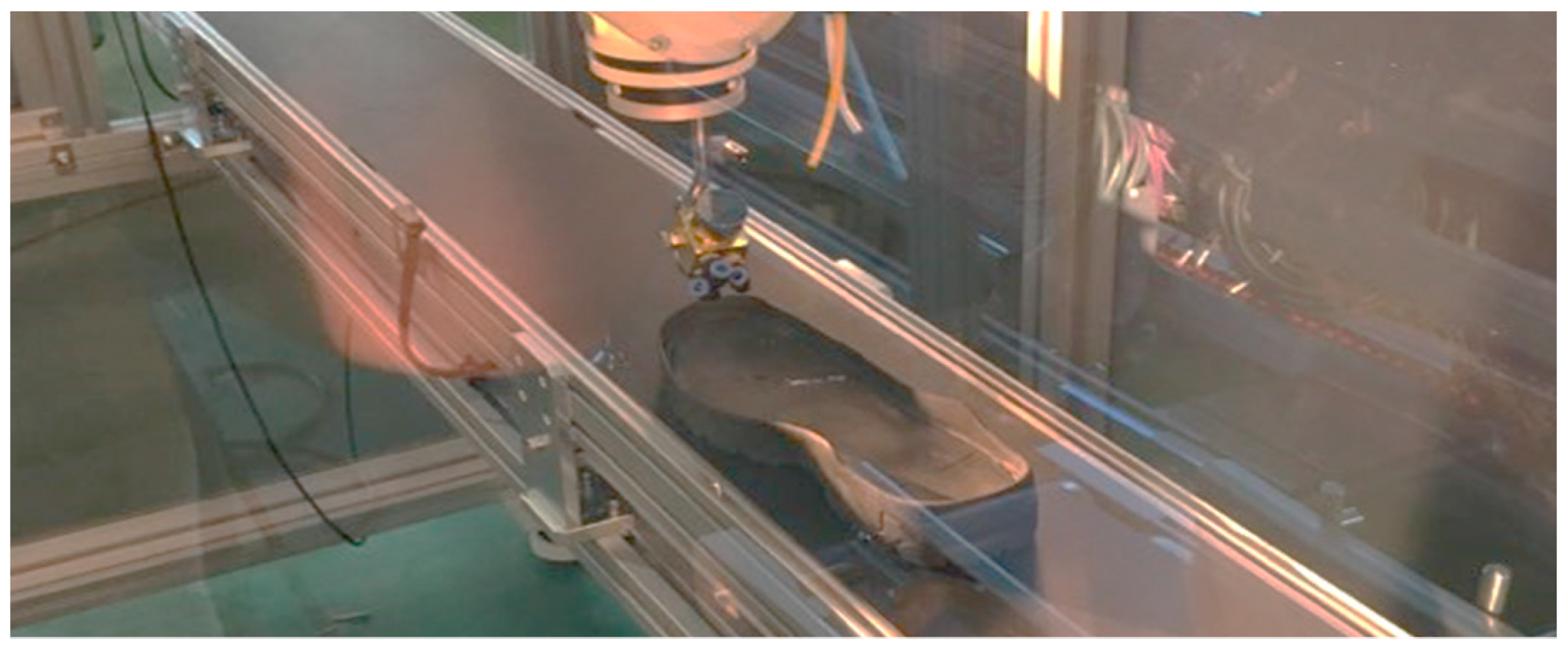
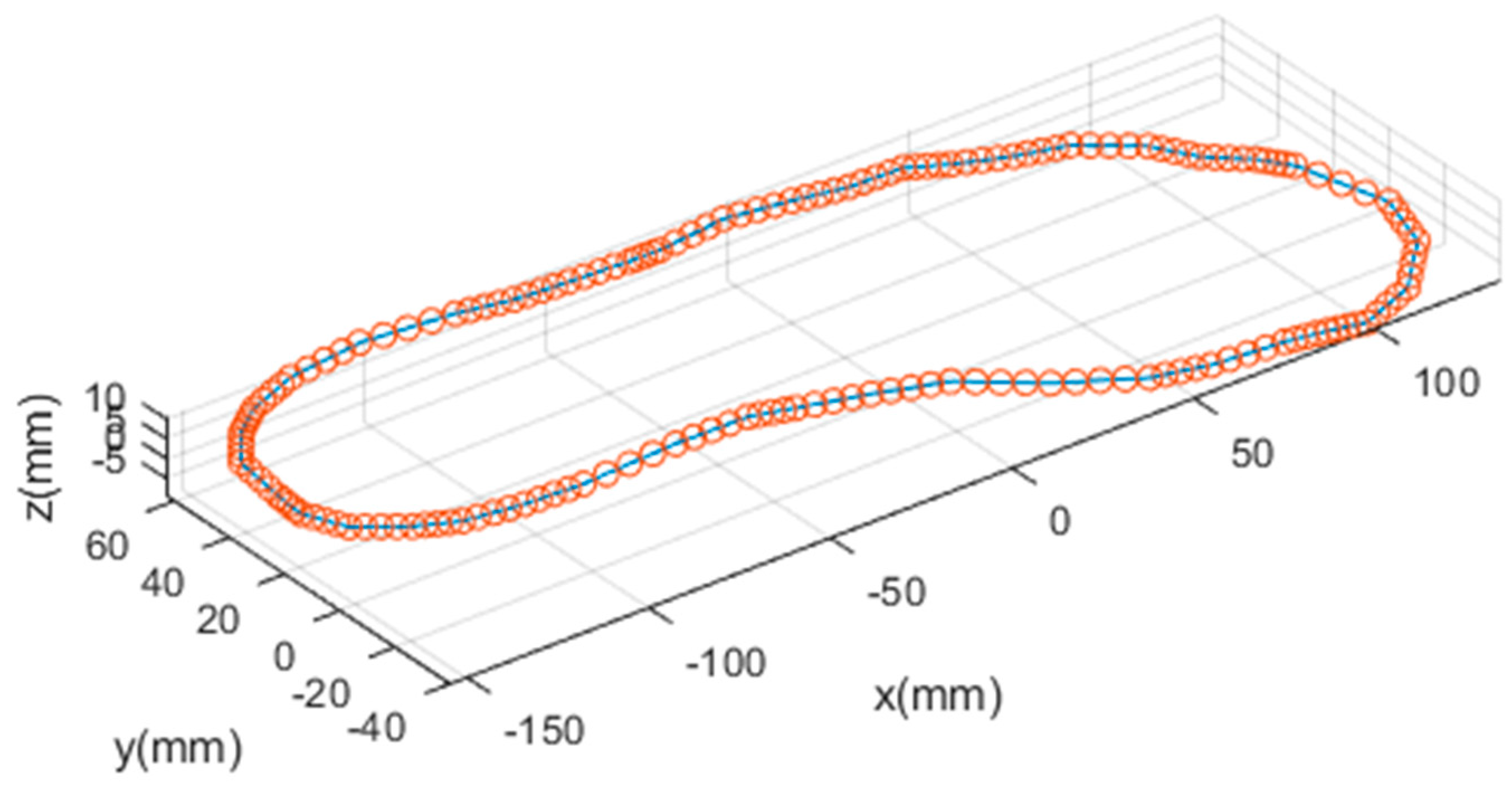
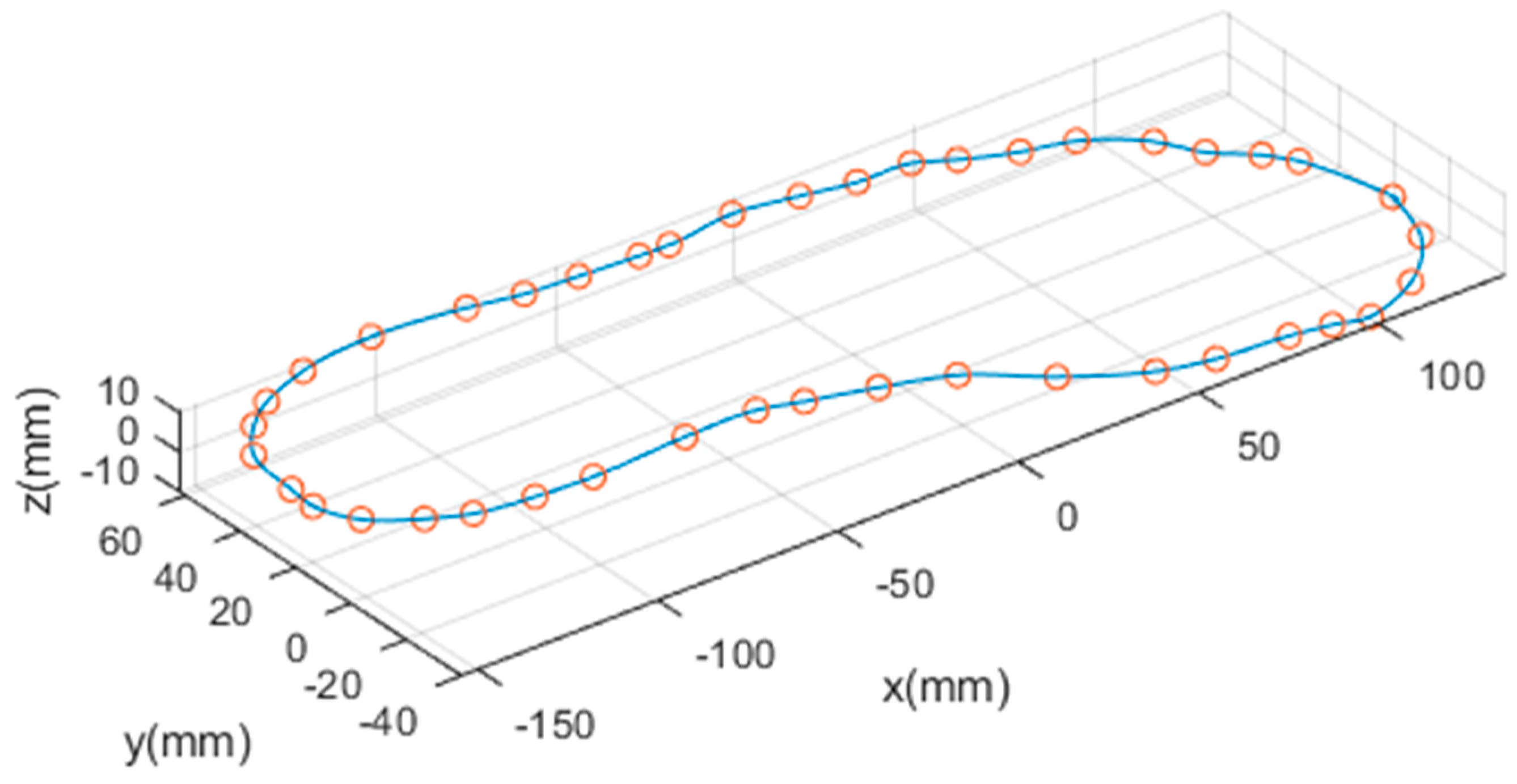
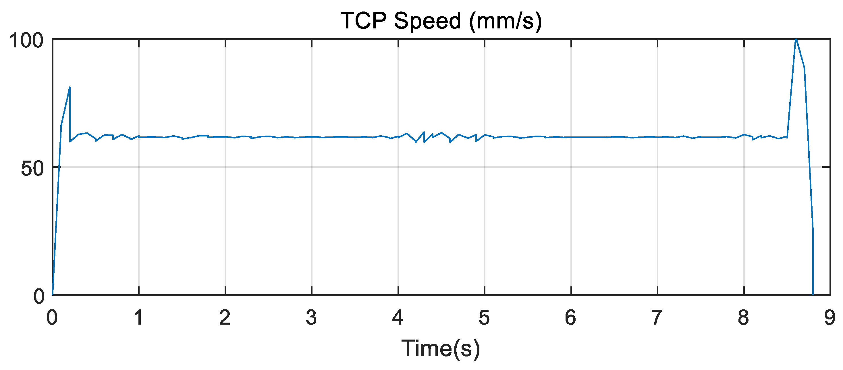
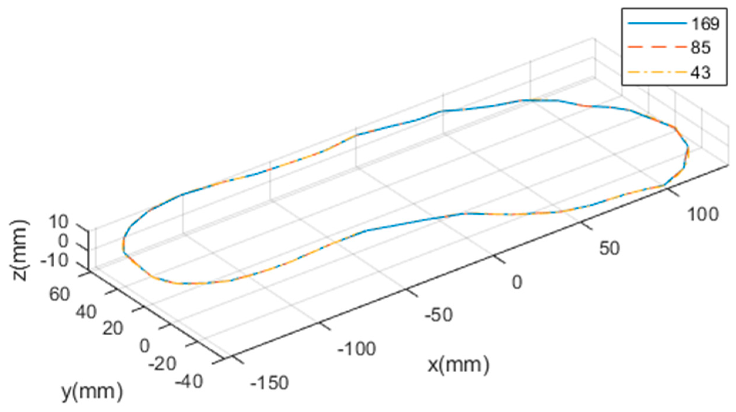
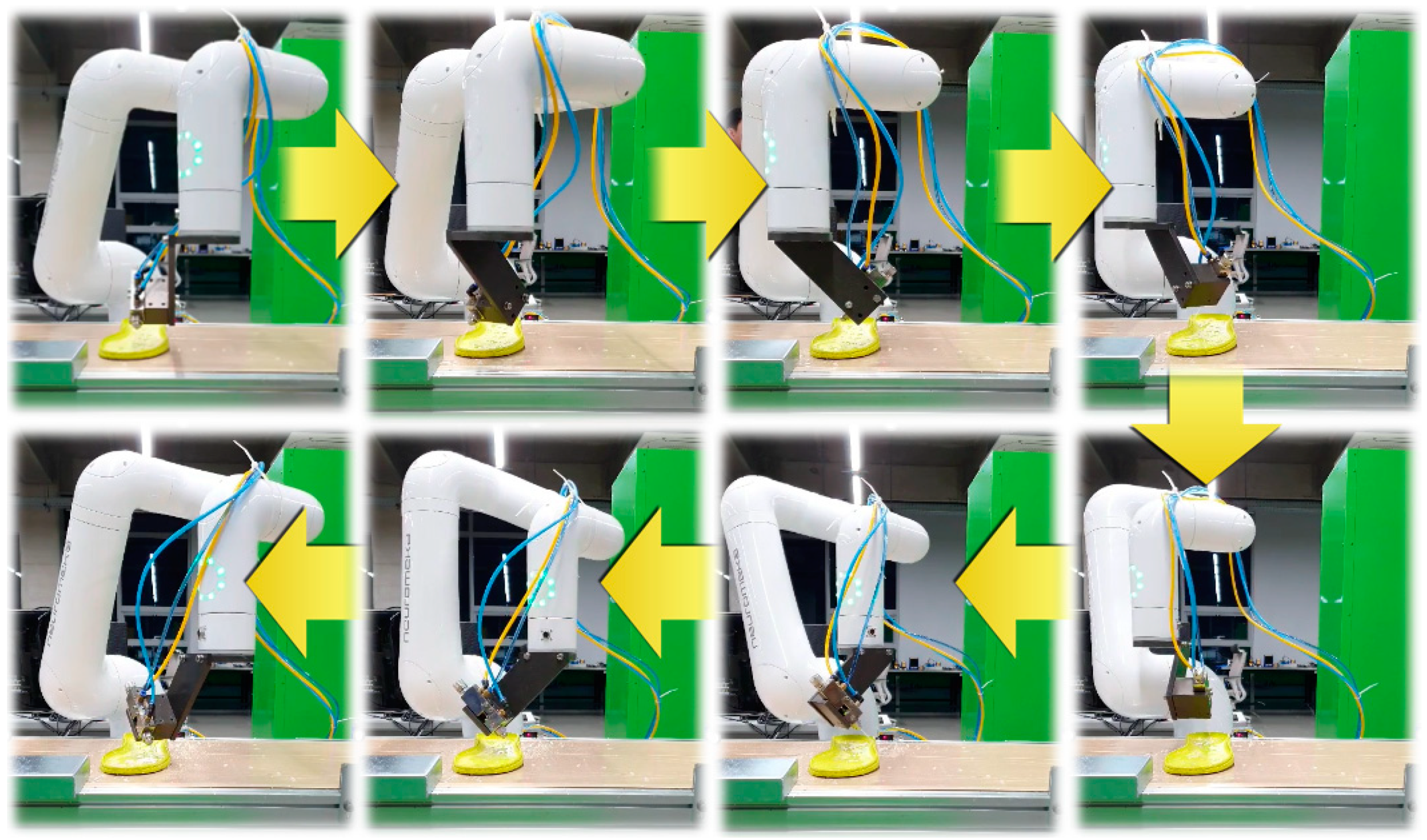
The proposed method is applicable to various robotic tasks requiring a robot to move continuously through multiple assigned points. To evaluate this, an experiment is executed to follow a 3-D curved contour. The target task is for the robot manipulator to dispense adhesive uniformly on the upper contour of the sole at a shoe manufacturing factory. The experimental results show that the proposed trajectory planning in the task space can be applied to the robotic task in the real manufacturing process.
Although the simulation and experimental results demonstrated that the proposed method was applicable to the robotic trajectory problem, this method could not guarantee the continuity of acceleration, and the curvature constraint in the cases where the knots consist of sharp curves should be considered. In the future, this method will be more applied to various complicated robotic tasks, and a method will also be studied to guarantee the continuity of acceleration and the constraints of physical curvature.


