Reformulating the Binary Masking Approach of Adress as Soft Masking

Abstract

Binary masking forms the basis for a number of source separation approaches that have been successfully applied to the problem of de-mixing music sources from a stereo recording. A well-known problem with binary masking is that, when music sources overlap in the time-frequency domain, only one of the overlapping sources can be assigned the energy in a particular time-frequency bin. To overcome this problem, we reformulate the classical pan-pot source separation problem for music sources as a non-negative quadratic program. This reformulation gives rise to an algorithm, called Redress, which extends the popular Adress algorithm. It works by defining an azimuth trajectory for each source based on its spatial position within the stereo field. Redress allows for the allocation of energy in one time-frequency bin to multiple sources. We present results that show that for music recordings Redress improves the SNR, SAR, and SDR in comparison to the Adress algorithm.

1. Introduction

Audio source separation is the problem of extracting sources that have been combined to form an observed audio mixture. Applications include speech enhancement and recognition [1] and hearing aid devices [2]. The separation of music sources from audio mixtures, namely Music Source Separation (MSS), has applications, such as (1) creating audio effects for the purpose of remixing and DJing; (2) automatic transcription of pitched instruments; and, (3) key-signature and chord-detection [3]. Time-Frequency (TF) two-channel methods for audio source separation have left an indelible mark on the field [4,5,6]. These methods are based on one or both of the following estimators, weighted, power-weighted or non-weighted relative attenuation, and/or delay estimation—a unifying framework for these estimators is given in [7]. We consider this mixing case, as most commercial music is in stereo format according to [3] (Formats such as 5.1 are not considered). Stereo mixtures allow for the spatial positioning of sources in a sound field; sources are perceived as originating from the left, centre or right, etc. Positioning is achieved via pan-pot mixing, which scales the contribution of each source to each channel. The relative delay between channels is less important for MSS [5] than speech source separation [4], which uses both relative delay and attenuation estimates to de-mix sources.

Music sources are typically sparse. This means that in the majority of TF bins the source has little energy. The source’s TF support is the remaining TF bins; they are small in number. Sparsity of the underlying sources coupled with independence of occurrence of sources should mean than in general sources do not overlap in TF—the success of Adress [5] bears testament to the conjecture that this is approximately true. However, two-channel TF methods do not generally work well in the TF bins where the sources overlap. Overlap arises for a number of reasons in MSS: harmonic signals are composed of a fundamental frequency and its harmonics; harmony causes a large degree of overlap in the frequency content of sources locally in time; percussive signals have a flatter spectrum than harmonic instruments, which increases the likelihood of them overlapping with harmonic instruments. In this paper, we consider what to do in the TF bins where the music sources do overlap, using a demixing algorithm, called Adress, which has seen wide-spread usage (since it was originally proposed in [5]), and has been the subject of recent analysis in [8]. Before we delve into our contribution, we chart the progress of Adress since it was originally proposed. The Adress algorithm was licensed for use in Sony’s Singstar on the Sony Playstation 3. It was then licensed to Riffstation, which was then sold to Fender and used by millions of users from 2012 to 2018. Our contribution is a soft-masked version of Adress, namely Redress, which seeks to remedy problem of what to do when sources overlap in TF.

The approaches above aim to separate sources by modeling the source positions [4,5,9]. They rely on binary masking and the assumption that only one source has significant energy in a given TF bin. Separation is achieved by assigning each TF bin to one source. This has been shown to be a special case of generalized Wiener filtering [10]. However, if sources overlap, only one source can be assigned the energy in that TF bin. An alternative to these approaches is methods that separate by modeling the sources. Approaches have also leveraged source-filter models in order to over-come the requirement for training of MSS systems. For example, to separate harmonic and percussive sources via tensor factorizations, the authors leveraged source-filter models for pitched instruments as well as constraints to encourage temporal continuity on pitched sources in [11]. Source-filter models were used in order to address the problem of pre-training, which they identified as a shortcoming of the approaches [12,13]. In addition, a disadvantage of pre-training approaches, such as [11], is that they can be processor and memory intensive. More recently, Deep Neural networks (DNNs) have been proposed in order to estimate non-negative masks, which are then applied to the TF representations of the audio mixture [14]. The advantage of TF approaches is that they make it possible to exploit the spectral structure of sources, however, approaches that operate in the time domain directly, such as [15,16], provide a good counter-point.

In contrast to stereo approaches, single-channel recordings do not provide information about the spatial position of sources. Non-negative Matrix Factorization (NMF) [17], which is generally applied to the magnitude spectrogram [18], relies on similar assumptions in terms of the sparsity of the sources in the TF domain to the approaches [4,5,9]. Redress considers the stereo TF instantaneous mixing model proposed in [5]. It does not involve pre-training but instead looks to exploit an initial estimate of the pan-position of the sources to simplify the separation problem by posing it as a non-negative quadratic program. For the squared Euclidean distance objective function, if one of NMF factors is fixed, the resulting problem is a nonnegative quadratic programme. One of the contributions of the present submission is that the Redress nonnegative quadratic programme is constructed by using pre-computed azimuth trajectories as one of the factors. A non-negative matrix factorization approach, where both factors were alternated, was proposed in [19]. This approach was only successful when the number of sources equalled (or was less than) the number of channels; its suitability was limited as there are generally more sources than sensors in practical applications. Redress then solves this optimization problem using a standard NMF-style one-sided update, whose performance is well understood. It works well when there are more sources than sensors.

This paper is organized, as follows. We introduce a simple pan-de-mixing problem to introduce Adress in Section 2. We introduce the main shorting-coming of the Adress approach using this problem. We then use this de-mixing problem to motivate Redress in Section 3. We describe our source reconstruction algorithm in Section 4. Finally, we evaluate the performance of Redress and compare it with Adress in Section 5.

2. Mixing Model

We define pan-mixing using a specific example to establish the notation used in the rest of this paper. Two continuous-time sound sources are considered, namely $s_1\left(t\right)$ and $s_2\left(t\right)$. Each source has two frequency components. The first source, $s_1\left(t\right)$, is composed of the frequencies $f_1=100$ Hz and $f_3=300$ Hz and the second source, $s_2\left(t\right)$, is composed of the frequencies $f_2=200$ Hz and $f_3=300$ Hz in Figure 1 (rows 1 and 2). Both sources are scaled by 2 to simplify notation, which yields the expressions

$$s_1\left(t\right)=2sin\left(2\pi f_{1}t\right)+2sin\left(2\pi f_{3}t\right),$$

(1)

$$s_2\left(t\right)=2sin\left(2\pi f_{2}t\right)+2sin\left(2s\pi f_{3}t\right).$$

(2)

A stereo mixture of these sources is produced by pan-mixing, by weighting the contribution of each source on the left channel and the right channel. The left and right channel signals, namely $x_1\left(t\right)$ and $x_2\left(t\right)$, produced using the weights $\alpha$ and $\gamma$, are defined as

$$x_1\left(t\right)=s_1\left(t\right)+\alpha s_2\left(t\right),$$

(3)

$$x_2\left(t\right)=\gamma s_1\left(t\right)+s_2\left(t\right),$$

(4)

and are illustrated in Figure 1 (rows 3 and 4). The weights lie in the intervals $0<\alpha <1$ and $0<\gamma <1$.

Appealing to the Fourier transform we can express the source signals, $s_1\left(t\right)$ and $s_2\left(t\right)$, more compactly in the frequency domain. The sources are denoted $S_1\left(f\right)$ and $S_2\left(f\right)$, where f denotes frequency and where, $\delta (·)$, is the delta function,

$$\begin{array}{cc}\hfill & S_1\left(f\right)=\delta (f-f_1)+\delta (f+f_1)+\delta (f-f_3)+\delta (f+f_3),\hfill \\ \hfill & S_2\left(f\right)=\delta (f-f_2)+\delta (f+f_2)+\delta (f-f_3)+\delta (f+f_3).\hfill \end{array}$$

(5)

As a consequence, the mixtures, $X_1\left(f\right)$ and $X_2\left(f\right)$, can also be expressed compactly as,

$$X_1\left(f\right)=\delta (f-f_1)+\delta (f+f_1)+\alpha \left(\delta (f-f_2)+\delta (f+f_2)\right)+(1+\alpha )\left(\delta (f-f_3)+\delta (f+f_3)\right),$$

(6)

$$X_2\left(f\right)=\gamma \left(\delta (f-f_1)+\delta (f+f_1)\right)+\left(\delta (f-f_2)+\delta (f+f_2)\right)+(1+\gamma )\left(\delta (f-f_3)+\delta (f+f_3)\right),$$

(7)

in the frequency domain.

These sources have been designed to include one frequency component that causes overlap in the mixtures and a second component that does not overlap in the mixtures.

2.1. Adress

In the Adress algorithm, the authors construct a frequency-azimuth plane as a first step towards separating the sources, $s_1\left(t\right)$ and $s_2\left(t\right)$, from the mixtures, $x_1\left(t\right)$ and $x_2\left(t\right)$. The frequency-azimuth plane is constructed by varying an independent variable, g, over the range, $0\le g\le 1$ and computing the magnitude of the difference between the two frequency domain mixtures. It is necessary to perform this scaling twice, where the roles of $X_1\left(f\right)$ and $X_2\left(f\right)$ are swapped, to preserve the symmetry of the frequency-azimuth plane. The gwo halves of the frequency-azimuth plane are produced by computing

$$A_1\left(f\right)=|X_1\left(f\right)-g{X}_2\left(f\right)|,$$

(8)

$$A_2\left(f\right)=|X_2\left(f\right)-g{X}_1\left(f\right)|.$$

(9)

Concatenating the components, $A_1\left(f\right)$ and $A_2\left(f\right)$, produces the entire frequency-azimuth plane, which is defined as

$$A\left(f\right)=\left[A_1\left(f\right)A_2\left(f\right)\right].$$

(10)

Given this concatenation of components and the role of g, which can assume values in the range $0\le g\le 1$, in each of these components, when we plot the frequency-azimuth plane we denote the range of g to be $-1\le g\le 1$ to capture this symmetry. In addition, we refer to the frequency-azimuth plane as the azimugram in the following sections. To de-mix the pan-mixed mixtures presented above, we only need to consider three frequency components $f_1,f_2$ and $f_3$. The azimugram can be defined in closed form for these three components.

$$A_1\left(f\right)=\left\{\begin{array}{cc}|1-g\gamma |,\hfill & \mathrm{when}f=f_1,\hfill \\ |\alpha -g|,\hfill & \mathrm{when}f=f_2,\hfill \\ \left|\right(1+\alpha )-g(1+\gamma \left)\right|,\hfill & \mathrm{when}f=f_3,\hfill \\ 0,\hfill & \mathrm{otherwise}.\hfill \end{array}\right.$$

(11)

$$A_2\left(f\right)=\left\{\begin{array}{cc}|\gamma -g|,\hfill & \mathrm{when}f=f_1,\hfill \\ |1-g\alpha |,\hfill & \mathrm{when}f=f_2,\hfill \\ \left|\right(1+\gamma )-g(1+\alpha \left)\right|,\hfill & \mathrm{when}f=f_3,\hfill \\ 0,\hfill & \mathrm{otherwise}.\hfill \end{array}\right.$$

(12)

In Equations (11) and (12) the gain satisfies the relationship $\left|g\right|\le 1$. The locations of nulls in the azimugram are important for source separation. For the three frequencies $f_1,f_2$ and $f_3$ the null locations are given by the gains

$$A\left(f\right)=0\mathrm{if}\left\{\begin{array}{cc}g=\gamma ,\hfill & \mathrm{when}f=f_1,\hfill \\ g=\alpha ,\hfill & \mathrm{when}f=f_2,\hfill \\ g=\frac{1+\alpha }{1+\gamma }\mathrm{or}\frac{1+\gamma }{1+\alpha }\mathrm{s}.\mathrm{t}.g\le 1\hfill & \mathrm{when}f=f_3.\hfill \end{array}\right.$$

(13)

The operation of the Adress algorithm is now summarized for discrete-time source signals which have been sampled at a rate which satisfies the Nyquist–Shannon sampling theorem. Adress computes windowed Discrete Fourier Transforms, $X_1\left(k\right)$ and $X_2\left(k\right)$, of the left and right channel mixture signals. The index k denotes the frequency bin indices, $k=0,1,\cdots ,K$. Figure 2 illustrates the positive frequencies of the magnitude spectra of the sources and mixtures, illustrating the frequency components that do overlap and those that do not. We use a set of gain values, $g=\left\{\frac{0}{\beta },\frac{1}{\beta },\cdots \frac{\beta }{\beta }\right\}$, where $\beta =\frac{M}{2}$, to construct the frequency-azimuth matrix, $\mathbf{A}\in {\mathbb{R}}^{K\times M}$. The matrix $\mathbf{A}$ is generally transformed in order to produce peaks at the locations of nulls in $\mathbf{A}$, yielding the matrix $\widehat{\mathbf{A}}$,

$$\widehat{\mathbf{A}}[k,m]=\left\{\begin{array}{cc}r\left[k\right],\hfill & \mathrm{if}\mathbf{A}[k,m]\equiv min\left\{\mathbf{A}\right[k,:\left]\right\}\hfill \\ 0,\hfill & \mathrm{otherwise},\hfill \end{array}\right.$$

(14)

where we introduce $r\left[k\right]=max\left\{\mathbf{A}\right[k,:\left]\right\}-min\left\{\mathbf{A}\right[k,:\left]\right\}$ to simplify the presentation. The motivation for this transformation is to simplify null/peak detection for the user. Figure 3 illustrates the resulting matrix, $\widehat{\mathbf{A}}$, for the two-source mixture introduced above. The peaks located at $\{f,g\}=\{100,-0.35\}$ and $\{200,0.4\}$ correspond to the frequency components of the sources that do not overlap. Recall that the sign of g is changed in order to distinguish between the right and left components of the azimugram (the value $-0.35$ is a gain of $0.35$ and the negative value indicates which TF mixture is scaled relative to the other one). Reconstruction of the component sources is achieved by assigning TF bins to sources depending on the location of the nulls in the frequency-azimuth plane using an azimuth subspace width parameter H.

2.2. Problem

A null is produced at the gain location, $g=\alpha$, in the frequency-azimuth plane by the mixture signals described above. This null corresponds to the source, $s_2\left(t\right)$, in the mixture, which excites the frequency $f_2=200$ Hz (cf. Figure 3). The source $s_2\left(t\right)$ also excites the frequency $f_3=300$ Hz. The location of the null in the $f_3=300$ Hz frequency band is generally not located at the same gain as the $f_2=200$ Hz component, e.g., $\alpha$. It is located at either $\frac{1+\alpha }{1+\gamma }$ or $\frac{1+\gamma }{1+\alpha }$ depending on the scale of $\alpha$ and $\gamma$. In Figure 3, this peak is located at $\frac{1+0.35}{1+0.4}\approx 0.96$. Note that we have used the scale value $0.35$ in the numerator and not $-0.35$ as the negative sign is used to facilitate plotting both components of the azimugram size-by-side in Figure 3. The scaling of the source signals in the mixtures produce another null at $g=\gamma$ at the frequency $f_1=100$ Hz. This null arises due to the source, $s_1\left(t\right)$, which is scaled by $\gamma$ in the second mixture $x_2$. A null is generally not located at the gain $g=\gamma$ in the $f_3=300$ Hz band. Co-occupation of the $f_3$ bin by the two source signals (which are scaled by different gains) causes the Adress algorithm to assign all of the energy of the frequency $f_3$ to one of the sources. The other source receives none of the energy. The decision on which source obtains the energy is made based on the distance of the location of the null of the $f_3$ component from the location of the nulls for the other frequency components of the $s_1$ and $s_2$ source signals. For example, in Figure 4, the recovered magnitude spectra for the two sources, obtained using the Adress algorithm are illustrated. The absence of the $f_3$ frequency component in one of the signals is a deficit. In this example, 50% of the frequency components of one of the sources will be missing and the other source will have a magnitude that is too large for that missing frequency component, because that source has incorrectly been assigned all of the energy in the $f_3$ frequency bin. This type of problem has been identified and called Frequency-Azimuth Smearing in [5], but it has not been solved.

Methods for trying to ensure that overlap does not happen rely on measuring the level of disjointness of sources in the TF domain; a common measure is Windowed Disjoint Orthogonality (WDO) [4,6]. WDO has been used in order to determine what parametrization of the Short-Time Fourier Transform (STFT) will give the most non-overlapping representation of the source signals in the TF mixtures [4,6]. We now present a solution to the problem of overlapping frequency components presented above that is motivated by re-considering the Adress mixing model.

3. Separation via Azimuth Trajectories

We introduce Redress, which uses azimuth trajectories to recover the source magnitude spectra.

Definition 1.

An azimuth trajectory is the response recorded in the frequency-azimuth matrix, $\mathbf{A}$, as a function of the gain, g, which has been varied over its range $0\le g\le 1$ in Equations (8) and (9).

We only consider the positive frequencies due to the symmetry of the TF representation. In the two-source case

$$X_1\left(f\right)=\delta (f-f_1)+\alpha \delta (f-f_2)+(1+\alpha )\delta (f-f_3),$$

(15)

$$X_2\left(f\right)=\gamma \delta (f-f_1)+\delta (f-f_2)+(1+\gamma )\delta (f-f_3).$$

(16)

In this discussion, one source dominates on the left-channel and the other dominates on the right-channel in order to address both scenarios. The first component of the azimugram is defined as:

$$\begin{array}{cc}\hfill A_1(f,m)& =\left|X_1\left(f\right)-g_m{X}_2\left(f\right)\right|\hfill \\ \hfill & =\left|(1-g_m\gamma )\delta (f-f_1)+(\alpha -g_m)\delta (f-f_2)+[(1-g_m\gamma )+(\alpha -g_m)]\delta (f-f_3)\right|\hfill \end{array}$$

(17)

The pan-mixing model does not delay sources and, thus, there is no relative delay between the two microphones. Each term can be expressed as a real-valued scalar, c, times a complex value, $z=(a+bj)$. The absolute value of the product $\left|cz\right|$ can be re-expressed as the product of the absolute value of the scalar times the absolute value of the complex value, $\left|cz\right|=\left|c\right|\left|z\right|$. Two cases warrant examination.

• When $f=f_1$ the azimugram can be simplified

  $$A_1(f_1,m)=|(1-g_m\gamma )\delta (f_1-f_1)|=|(1-g_m\gamma )\left|\right|\delta (f_1-f_1)|,$$

  (18)

  as the product of $s_1$’s azimuth trajectory $h_1\left(g\right)=\left|(1-g_m\gamma )\right|$ and $s_1$’s spectral content $\left|\delta \right(f_1-f_1\left)\right|$ at that frequency.
• When $f=f_3$ the azimugram can be expressed as

  $$A_1(f_3,m)=|(1-g_m\gamma )+(\alpha -g_m)\left|\right|\delta (f_3-f_3)|,$$

  (19)

  however, from the triangle inequality, it holds that

  $$\left|\right(1-g\gamma )+(\alpha -g\left)\right|\le \left|\right(1-g\gamma \left)\right|+\left|\right(\alpha -g\left)\right|.$$

  (20)
  Expressing this portion of the azimugram as the product of source trajectories, $h_1\left(g\right)=\left|(1-g_m\gamma )\right|$ and $h_2\left(g\right)=\left|(\alpha -g_m)\right|$, and their corresponding source spectral content is an approximation.

For mixtures consisting of an arbitrary number of sources, who have, in turn, different magnitudes in each of the TF bins, the error introduced by assuming the inequality is in fact equality in Equation (20) depends on the location of the sources that are occupying the bins, the values of $\alpha$ and $\gamma$ in Equation (20) and also the magnitude spectra in those frequency bins.

Continuing with discrete TF representations of the signals, and cognisant of the approximation introduced by the triangle inequality, we approximate the azimugram component ${\mathbf{A}}_1(k,m)$ with the following factorization in the two source case. The two matrices, $\mathbf{W}$ and $\mathbf{H}$, are defined as

$$\begin{array}{c}{\mathbf{A}}_1\approx \left[\begin{array}{cc}⋮& ⋮\\ {\delta }_{k{k}_1}& 0\\ ⋮& ⋮\\ 0& {\delta }_{k{k}_2}\\ ⋮& ⋮\\ {\delta }_{k{k}_3}& {\delta }_{k{k}_3}\\ ⋮& ⋮\end{array}\right]\times \left[\begin{array}{cccc}\left|\right(1-g_0\gamma \left)\right|& \left|\right(1-g_1\gamma \left)\right|& \cdots & |(1-g_{\frac{M}{2}}\gamma )|\\ \left|\right(\alpha -g_0\left)\right|& \left|\right(\alpha -g_1\left)\right|& \cdots & |(\alpha -g_{\frac{M}{2}})|\end{array}\right]\end{array}$$

(21)

where the bins $k_1$, $k_2$, and $k_3$ correspond to the frequencies $f_1,f_2$, and $f_3$, and ${\delta }_{k{k}_i}$ is the Kronecker delta. A similar factorization can be constructed for the other component of the azimugram ${\mathbf{A}}_2(k,m)$.

4. Reconstruction

In the case of an arbitrary number of sources, R, the azimugram $\mathbf{A}\in {\mathbb{R}}_{+}^{K\times M}$ is approximated by the product of the source magnitude TF Spectra in the $\tau$-th time window times the azimuth trajectory of that source. The azimuth trajectories matrix is pre-computed. It is formed by adding a row to the matrix $\mathbf{H}\in {\mathbb{R}}_{+}^{R\times M}$ for each source, given estimates of the azimuths of each source, $a=\{a_1,a_2,\cdots ,a_R\}$. These azimuths are either selected by the user (cf. [5]) or estimated while using a relative attenuation estimator (cf. [7]). If the r-th source dominates on one channel the trajectory is

$${\mathbf{h}}_r=\left[\cdots ,|1-g_2{a}_r|,|1-g_1{a}_r|,1,|-a_r-g_1|,|-a_r-g_2|,\cdots \right].$$

(22)

If the r-th source dominates on the other channel the trajectory is

$${\mathbf{h}}_r=\left[\cdots ,|-a_r-g_2|,|-a_r-g_1|,1,|1-g_1{a}_r|,|1-g_2{a}_r|,\cdots \right].$$

(23)

The azimuth trajectories matrix, given the azimuth estimates a, is

$$\mathbf{H}={\left[\begin{array}{cccc}{\mathbf{h}}_1& {\mathbf{h}}_2& \cdots & {\mathbf{h}}_R\end{array}\right]}^T.$$

(24)

The recovery of the magnitude spectra of the source signals is achieved by solving the non-negative quadratic programme

$$\begin{array}{cc}\hfill {\min }_{\mathbf{W}}& \left|\right|\mathbf{A}-{\mathbf{W}\mathbf{H}\left|\right|}_2^2,\hfill \\ \hfill \mathrm{subject}\mathrm{to}& {\mathbf{W}}_{k,m}\ge 0.\hfill \end{array}$$

(25)

where $\mathbf{W}\in {\mathbb{R}}_{+}^{M\times R}$ for the azimugram computed for the $\tau$-th window of the analyzed mixtures $X_1[k,\tau ]$ and $X_2[k,\tau ]$. We use the update proposed by Lee and Seung in [17], e.g., $\mathbf{W}\leftarrow \mathbf{W}\odot \mathbf{A}{\mathbf{H}}^T\oslash \mathbf{W}\mathbf{H}{\mathbf{H}}^T$. The resulting $\mathbf{W}$ factor is approximately equal to the source magnitude TF spectra:

$$\mathbf{W}\approx \left[\begin{array}{cccc}|S_1[1,\tau ]|& |S_2[1,\tau ]|& \cdots & |S_R[1,\tau ]|\\ |S_1[2,\tau ]|& |S_2[2,\tau ]|& \cdots & |S_R[2,\tau ]|\\ ⋮& ⋮& ⋮& ⋮\\ |S_1[K,\tau ]|& |S_2[K,\tau ]|& \cdots & |S_R[K,\tau ]|\end{array}\right].$$

(26)

The reconstruction of the discrete-time r-th source is achieved by forming an estimate of its entire magnitude TF Spectrum, by taking the r-th column from each estimate of $\mathbf{W}$ and forming

$$\widehat{\mathbf{S}}=\left[\begin{array}{ccccc}|S_r[1,1]|& |S_r[1,2]|& \cdots & |S_r[1,\tau ]|& \cdots \\ |S_r[2,1]|& |S_r[2,2]|& \cdots & |S_r[2,\tau ]|& \cdots \\ ⋮& ⋮& ⋮& ⋮\\ |S_r[K,1]|& |S_r[K,2]|& \cdots & |S_r[K,\tau ]|& \cdots \end{array}\right].$$

(27)

We use the mixture phase to reconstruct the discrete-time source. Algorithm 1 summarizes the workflow of the Redress algorithm.

Figure 5 illustrates the time-frequency magnitude spectra of both sources learned using Redress. Both sources are now assigned a frequency component in the $f_3=300$ Hz bin. In comparison Adress is unable to assign energy in the $f_3=300$ Hz bin to both source signals. Figure 6 illustrates the separated azimugrams which result from the Redress approach. In summary, the factorization of the azimugram learned by Redress allows both of the component azimugrams to have peaks at the correct gain for the 300 Hz component.

Algorithm 1: Summary of the Redress Algorithm

Result: Separated sources $s_1,s_2,\cdots$

Compute the STFT of both channels, $x_1$ and $x_2$;

Compute the frequency azimuth plane by constructing $A_1$ and $A_2$ (Equations (8) and (9));

Form the azimuth trajectory matrix, $\mathbf{H}$, using Equations (22)–(24);

Recover the sources by solving the NQP in Equation (25);

Extract the sources from the columns of the source magnitude TF Spectra matrix, $\mathbf{W}$, matrix in Equation (26);

Reconstruct the source magnitude spectra using Equation (27);

Use the mixture phase to reconstruct the discrete-time sources;

5. Evaluation

We generated stereo pan-mixed mixtures using up to four of the original stems, (bass, drums, other instruments, and vocals) provided in the Demixing Secret Dataset (DSD) in order to evaluate the performance of Redress [20]. According to [3], the DSD dataset has gained traction as an evaluation dataset for source separation problems. Evaluation was carried out using an FFT size of 4096 samples, with a hopsize of 2048 samples, and a sampling frequency of $44.1$ kHz in order to be consistent with [5]. The analysis window used was a Hamming window. We ran the Redress algorithm for 100 iterations. All of the mixtures were created by down-mixing any stereo stems to mono and then remixing them with two, three of four different azimuth positions depending on the number of sources in the mixture. The source-count parameter, R, of Redress was set to the number of sources in the mixture. For both Adress and Redress, we assumed the azimuths a were known. Both Adress and Redress were implemented in Matlab 2018b (9.5.0.944444 (R2018b), Mathworks, Natick, MA, USA).

The purpose of this evaluation was to test the hypothesis that Redress could improve the source estimates achieved by a binary masking approach when the sources overlapped in the TF domain. We increased the number of source signals present in the mixtures from two to four in order to vary the level of overlap in the TF domain. Four was the maximum number of sources available for each track in the DSD dataset. The baseline method used in our comparison was the Adress algorithm, which uses a binary masking approach for separation.

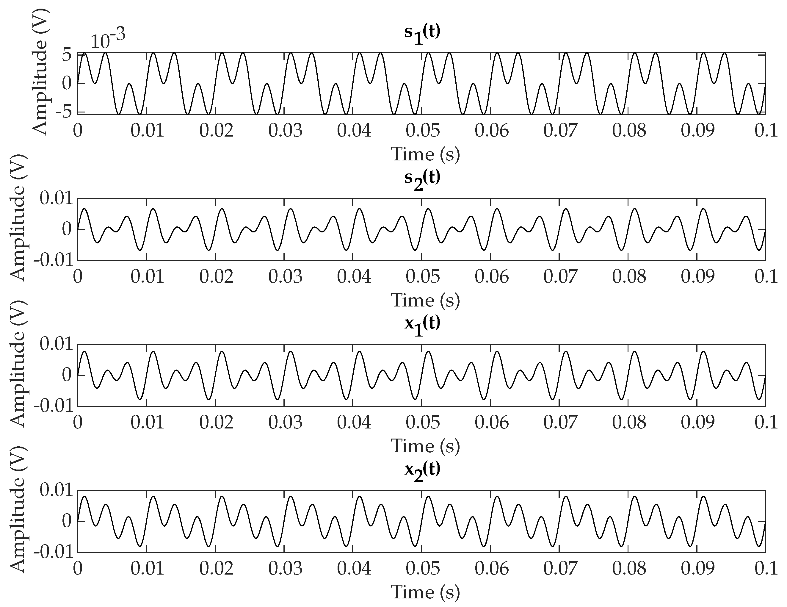
5.1. Separation Example: Redress

We present a separation example using a four-source mixture and the Redress algorithm. Figure 7 illustrates a 10 s excerpt of the original four source components of Patrick Talbot’s “Set Me Free” from the DSD dataset. Two components are panned left and the other two components are panned right. Figure 8 illustrates the estimates of these sources achieved by Redress. The separations are of high quality; there are very few visual differences between the original sources and the estimates of them. The bass, other instruments, and voice waveforms contain little or no evidence of the percussion/drums events. Similarly, the drums waveform contains little or none of the components of the harmonic instruments.

We illustrate the magnitude TF representations of the original sources and estimates of these sources signals in Figure 9 and Figure 10. The drums have significant spectral energy from 0–15 kHz. The voice and instruments are compactly supported in the range 0–5 kHz. Both the other instruments and the voice have energy in the frequency range 5–15 kHz. This energy overlaps with much of the drums’ energy. Figure 9 illustrates that estimates of the sources: drums, voice, and other instruments, have energy in this range, which illustrates the benefit of Redress over a binary masking approach. The bass and other instruments have been assigned less of this energy. In a binary mask-based source separation approach, only one source can be assigned energy in a TF bin, which can cause the resulting magnitude TF spectra to have gaps if that energy is assigned to another source.

On listening to the recovered waveforms, we conclude that the quality is high. There are some audible artifacts where ideal separation is not achieved, which we now describe. Some traces of the higher frequencies of the drums can be heard on one other estimated source, the other instruments waveform. Some components of the voice waveform are present in the bass waveform. However, the drums waveform is very good; both the low and high frequency components are present. Similarly, the voice waveform is excellent in spite of the fact that some of the voice higher frequency energy is assigned to the bass. This experiment suggests that TF bins can be assigned to multiple source estimates, which is not possible using binary masking approaches. The Redress algorithm seeks to minimize the reconstruction error and, to do this, it may assign the energy in TF to multiple sources. From the triangle inequality (Equation (20)), the factorization that we have proposed is not exact. It is exact when sources are disjoint in TF; it is approximately correct when sources are not disjoint, and the quality of the approximation depends on the magnitude of the sources sharing the TF and their panning weights. We now investigate the approximation achieved by Redress and the binary masking approach used by Adress.

5.2. Overlapping Sources in TF

Table 1. Av. SNR (dB) of the source estimates: 2-source mixtures.

	Bass	Drums	Other Instruments	Voice
Redress	11.8667	14.5693	-	-
Adress	10.7585	11.4251	-	-
Redress	-	13.3784	15.7878	-
Adress	-	11.4412	12.1051	-
Redress	-	-	10.4634	13.4975
Adress	-	-	9.3739	10.3778
Redress	13.0597	-	-	16.4422
Adress	10.1297	-	-	8.7984

,

Table 2. Av. SNR (dB) of the source estimates: 3-source mixtures.

	Bass	Drums	Other Instruments	Voice
Redress	9.8884	10.8795	8.7282	-
Adress	10.0437	8.6279	7.4703	-
Redress	9.0305	11.5192	-	8.8494
Adress	9.0694	9.7596	-	7.3313
Redress	10.7974	-	10.7052	8.2186
Adress	10.8326	-	8.5726	7.7733
Redress	-	10.1772	9.6942	7.6430
Adress	-	10.1582	7.8717	7.0842

and

Table 3. Av. SNR (dB) of the source estimates: 4-source mixtures.

	Bass	Drums	Other Instruments	Voice
Redress	6.0854	8.7291	5.8795	4.1330
Adress	5.2224	7.3386	5.0702	6.8377

illustrate the Signal-to-Noise Ratios (SNRs) of the source estimates achieved over a range of mixing scenarios. In the first case, two of the four sources are mixed and the other two sources are not included in the mixtures (cf. Table 1). In Table 1, the SNRs for estimates of the two sources in the mixtures are indicated and a dash indicates that the corresponding source was not present in the mixture. Similarly, in the second case, three of the four sources are included in the mixture (cf. Table 2) and in the final case all four sources are included Table 3. In general, the SNRs of the estimated sources decreases when the number of sources increases, which can be attributed to the increased TF overlap of the sources when more sources are present. This first result demonstrates that Redress is affected by increased TF overlap. On average, Redress improves the SNR of the reconstructed sources by 3, 1 and $0.1$ dB in the two, three, and four sources mixtures in comparison with the sources recovered by Adress. Note that the results for the Adress algorithm are improved by artificial means in these experiments. When the sources are reconstructed by Adress, we have the choice of reconstructing from the left channel or the right channel. The choice of the left channel over the right channel has a significant bearing on the SNR of the result. To compare Redress with the best possible Adress result, we use knowledge of the original sources and estimate the SNR for sources, which have been estimated from both channels and choose the maximum value. In the Redress case, we do not leverage knowledge about the true sources in order to improve the estimate achieved. Even with this advantage, Redress outperforms Adress in terms of the SNR estimates of the recovered sources. In these experiments, the Adress algorithm was parameterized with 201 equally spaced azimuth positions and a target azimuth range of 20 azimuth positions. These parameters were used in the evaluation of Adress in [8].

Figure 11 displays boxplots of the measurements obtained for each mixture class, e.g., 2, 3, or 4 sources while using the MATLAB toolbox BSS EVAL [21]. The measurements considered included (1) the Source-to-Distortion Ratio (SDR) which we interpret as a global quality assessment; (2) the Source-to-Artifacts Ratio (SAR) which in this case is related to the level of musical noise introduced into the source estimates; and finally, (3) the Source-to-Interference Ratio (SIR), which measures the interference from other sources in the estimated sources. In general, all of the measurements decreased as the number of sources increased due the increasing likelihood of sources overlapping in TF. Adress yielded higher Source-to-Interference Ratios (SIR) than Redress. This is unsurprising, as Redress was developed to be able to assign contributions in TF bins to multiple sources. This has the consequence of decreasing SIRs achieved by it when compared to the binary masking approach, Adress. A disadvantage of binary masking approaches is that the aggressive way that TF bins are assigned to one source only typically causes the level of distortion and artefacts that are introduced into the source estimates to increase. Figure 11 illustrates that Redress generally yields higher SDRs and SARs than Adress. The SDR and SAR capture the overall sound quality of the separated source signals. Artifacts—mainly musical noise—are reduced by Redress’s ability to assign TF bins to multiple sources. As a consequence of this, the TF spectra of the sources tend to have fewer isolated bins with energy. This is evident from the TF representations of the separated sources in Figure 9.

5.3. Discussion and Future Work

One of the main contributions of this paper was to reformulate the binary masking approach of Adress as a soft masking problem and then to solve this problem using a nonnegative quadratic programme. The SAR, SNR, and SDR scores achieved by Redress were better than the Adress algorithm under the condition that the number of sources was known. In the experiments, not all sources were playing at the same time and with the same intensity. The challenge of time varying numbers of sources was also faced by the Adress algorithm. It would be interesting to consider how both algorithms could adaptively set the number of sources in order to improve their performance when the assumed number of sources was incorrect. In many cases, the Adress algorithm implementation allows for the user to choose target azimuths for sources as a way to solve this problem. The Redress algorithm could also benefit from similar user supervision.

Regarding the SIR performance of both algorithms, the SIR performance was better for the original Adress algorithm than the proposed algorithm, Redress. This would imply that Adress provides better separation of the sources. Thus, Redress seems to make separation worse, but the overall sound quality better. It is important to consider the target application of Redress. The separated sources learned by Adress are typically re-mixed in order to reduce the effects of the musical noise introduced by the algorithm as a consequence of the binary masking approach it takes to source separation. In effect, Adress separates the sources and then remixes the sources in order to reduce the artifacts and distortions (measured using SARs and SDRs) that arise as a consequence of the uncompromising nature of binary masking.

One of the motivations for the interest in Adress was its low computation complexity and, thus, the possibility of implementing it in real-time. In many cases, Adress is not used in real-time, as the user selects an appropriate azimuth based on an inspection of a simplified form of the azimugram. In comparison, our implementation of Redress in the current paper uses 100 iterations of an NMF-style update, which was proposed by Lee and Seung, e.g., $\mathbf{W}\leftarrow \mathbf{W}\odot \mathbf{A}{\mathbf{H}}^T\oslash \mathbf{W}\mathbf{H}{\mathbf{H}}^T$, in order to reconstruct the source signals. A first analysis of the computational complexity of the Redress approach can be summarized as follows. We only consider computations that are different to those computed by Adress. The matrix $\mathbf{H}$ can be pre-computed by the system for all possible azimuths. Therefore, it can be stored as a look-up table and so it does not pose a computational burden for a real-time implementation of the approach. Similarly, the matrix product, $\mathbf{H}{\mathbf{H}}^T$, can be computed off-line and stored in a look-up table for run-time. The computational cost of Redress involves two matrix products, $\mathbf{A}{\mathbf{H}}^T$ and $\mathbf{W}\mathbf{H}{\mathbf{H}}^T$, and one matrix element-wise product and division. The complexity of these terms is set by the size of the FFT, the number of sources to detect and the number of azimuth positions. We posit that this computational load should not be a barrier to implementing Redress in a manner that has the same responsive performance as Adress, even when this update is run in an iteration for 100 steps.

6. Conclusions

In this paper, we investigated whether it was possible to use pre-computed source azimuth trajectories as activation functions in a pan-pot de-mixing problem. We showed that by doing so, the de-mixing problem could be reformulated as a Non-negative Quadratic Program which allowed the Redress source separation algorithm to assign energy to multiple sources who shared a TF bin. The results suggested that Redress decreased the artefacts that were introduced into source estimates. This came at the cost of increasing the level of interference from other sources in those estimates. Redress has a number of advantages that we summarize now. The problem that binary masking had with regard to the $f_3$ frequency, the shared frequency bin in the motivating example, in Section 2, has been addressed. Redress allocates some of the energy of the mixture at $f_3$ Hz to both sources. The allocation is generally not the correct solution, but it is preferable to allocating all of the energy to one source, and none to the other sources. With regard to the parameter selection that is required for Adress, we selected the value H, which is an azimuth range used to partition the frequency-azimiuth plane, by testing a number of different settings for the best result. Redress only required that the number of sources R be set for it to out-perform Adress. No other testing to optimize parameters was required. In addition, using Redress, there was no ambiguity about which channel should be used to de-mix the sources. When sources are reconstructed, the Adress algorithm can use either mixture to recover the source signals. In our experiments, we reconstructed the sources using both mixture magnitude TF spectra and then picked the one with the best SNR, SIR, SDR, or SAR, depending on the context. Redress estimated the source magnitude spectra using both mixtures and so no choice is available, or required. Finally, Redress outperformed Adress in terms of the achieved SNR, SDR, and SAR for mixtures consisting of two to four sources.

References

1. Barker, J.; Watanabe, W.; Vincent, E.; Trmal, J. The fifth chime speech separation and recognition challenge: Dataset, task and baselines. arXiv 2018, arXiv:1803.10609. [Google Scholar]
2. Wang, D. Time-frequency masking for speech separation and its potential for hearing aid design. Trends Amplif. 2008, 12, 332–353. [Google Scholar] [CrossRef] [PubMed] [Green Version]
3. Cano, E.; FitzGerald, D.; Liutkus, A.; Plumbley, M.; Stöter, F. Musical Source Separation: An Introduction. IEEE Signal Process. Mag. 2019, 36, 31–40. [Google Scholar] [CrossRef]
4. Yilmaz, O.; Rickard, S. Blind separation of speech mixtures via time-frequency masking. IEEE Trans. Signal Process. 2004, 52, 1830–1847. [Google Scholar] [CrossRef]
5. Barry, D.; Lawlor, B.; Coyle, E. Sound Source Separation: Azimuth Discrimination and Resynthesis. In Proceedings of the 7th International Conference on Digital Audio Effects, Naples, Italy, 5–8 October 2004. [Google Scholar]
6. de Fréin, R.; Rickard, S.T. The Synchronized Short-Time-Fourier-Transform: Properties and Definitions for Multichannel Source Separation. IEEE Trans. Signal Process. 2011, 59, 91–103. [Google Scholar] [CrossRef] [Green Version]
7. de Fréin, R.; Rickard, S.T. Power-Weighted Divergences for Relative Attenuation and Delay Estimation. IEEE Signal Process. Lett. 2016, 23, 1612–1616. [Google Scholar] [CrossRef] [Green Version]
8. Barry, D. Real-Time Sound Source Separation for Music Applications. Ph.D. Thesis, Technological University Dublin, Dublin, Ireland, 2019. [Google Scholar] [CrossRef]
9. FitzGerald, D.; Liutkus, A.; Badeau, R. Projection-Based Demixing of Spatial Audio. IEEE/ACM Trans. Audio Speech Lang. Process. 2016, 24, 1560–1572. [Google Scholar] [CrossRef]
10. Duong, N.; Vincent, E.; Gribonval, R. Under-Determined Reverberant Audio Source Separation Using a Full-Rank Spatial Covariance Model. IEEE Trans. Audio Speech Lang. Process. 2010, 18, 1830–1840. [Google Scholar] [CrossRef] [Green Version]
11. Fitzgerald, D.; Coyle, E.; Cranitch, M. Using Tensor Factorisation Models to Separate Drums from Polyphonic Music. In Proceedings of the International Conference on Digital Audio Effects (DAFX09), Como, Italy, 1–4 September 2009; pp. 1–4. [Google Scholar]
12. Yoshii, K.; Goto, M.; Okuno, H.G. Drum Sound Recognition for Polyphonic Audio Signals by Adaptation and Matching of Spectrogram Templates With Harmonic Structure Suppression. IEEE Trans. Audio Speech Lang. Process. 2007, 15, 333–345. [Google Scholar] [CrossRef] [Green Version]
13. Gillet, O.; Richard, G. Transcription and Separation of Drum Signals From Polyphonic Music. IEEE Trans. Audio Speech Lang. Process. 2008, 16, 529–540. [Google Scholar] [CrossRef] [Green Version]
14. Wang, D.; Chen, J. Supervised Speech Separation Based on Deep Learning: An Overview. IEEE/ACM Trans. Audio Speech Lang. Process. 2018, 26, 1702–1726. [Google Scholar] [CrossRef] [PubMed]
15. Luo, Y.; Mesgarani, N. TaSNet: Time-Domain Audio Separation Network for Real-Time, Single-Channel Speech Separation. In Proceedings of the 2018 IEEE International Conference on Acoustics, Speech and Signal Processing (ICASSP), Calgary, AB, Canada, 15–20 April 2018; pp. 696–700. [Google Scholar]
16. Luo, Y.; Mesgarani, N. Conv-TasNet: Surpassing Ideal Time–Frequency Magnitude Masking for Speech Separation. IEEE/ACM Trans. Audio Speech Lang. Process. 2019, 27, 1256–1266. [Google Scholar] [CrossRef] [PubMed] [Green Version]
17. Lee, D.; Seung, H. Algorithms for Non-Negative Matrix Factorization; MIT Press: Cambridge, MA, USA, 2000; pp. 556–562. [Google Scholar]
18. Virtanen, T. Monaural Sound Source Separation by Nonnegative Matrix Factorization with Temporal Continuity and Sparseness Criteria. IEEE Trans. Audio Speech Lang. Process. 2007, 15, 1066–1074. [Google Scholar] [CrossRef] [Green Version]
19. de Fréin, R. Remedying Sound Source Separation via Azimuth Discrimination and Re-synthesis. In Proceedings of the Irish Signals and Systems Conference, Donegal, Ireland, 11–12 June 2020. [Google Scholar]
20. Liutkus, A.; Stöter, F.; Rafii, Z.; Kitamura, D.; Rivet, B.; Ito, N.; Ono, N.; Fontecave, J. The 2016 Signal Separation Evaluation Campaign. In Latent Variable Analysis and Signal Separation; Tichavský, P., Babaie-Zadeh, M., Michel, O., Thirion-Moreau, N., Eds.; Springer: Cham, Switzerland, 2017; pp. 323–332. [Google Scholar]
21. Vincent, E.; Gribonval, R.; Fevotte, C. Performance measurement in blind audio source separation. IEEE Trans. Audio Speech Lang. Process. 2006, 14, 1462–1469. [Google Scholar] [CrossRef] [Green Version]
Figure 1. Rows 1 and 2 illustrate two sources signals. Source 1, s 1 ( t ) , has a 100 Hz and a 300 Hz frequency component. Source 2, s 1 ( t ) , has a 200 Hz and a 300 Hz frequency component. Rows 3 and 4 illustrate pan-mixed mixtures of the sources, x 1 ( t ) and x 2 ( t ) .
Electronics 09 01373 g001
Figure 2. The magnitude spectra of the source signals, s 1 and s 2 , and mixtures, x 1 and x 2 , are illustrated for 155 analysis windows and over the frequency range 0 f 1000 Hz.
Electronics 09 01373 g002
Figure 3. The frequency-azimuth plane constructed for the mixtures x 1 and x 2 are illustrated for the frequency range 0 f 500 Hz and for gains (or azimuths) 1 g 1 . Peaks at are positioned at the gains 0.35 and 0.4 for the s 1 and s 2 at frequencies 100 Hz and 200 Hz, respectively. The 300 Hz component of s 1 and s 2 does not appear as two separate peaks, but as one peak with a gain that is inconsistent with s 1 and s 2 ’s azimuth.
Electronics 09 01373 g003
Figure 4. The reconstruction achieved by Adress using an azimuth subspace width of H = 65 azimuths is illustrated. We use 100 azimuths for the LHS component and 100 azimuths for the RHS component of the azimugram. In the case that H = 65 , only one de-mixed spectra contains the 300 Hz frequency component. The value H = 65 is chosen so that the peak at the frequency f 3 is assigned to the nearest source. The peak at 0.96 is approximately 61 azimuths away from the peak at 0.35 and so it is assigned to the source s 1 . The peak at 0.4 is 75 azimuths away from the peak at 0.35 and so the f 2 frequency component is not assigned to the s 1 source. Choosing a smaller H might result in the f 3 component not being assigned to either source. Choosing H can be a challenge. Secondly, the magnitudes of the components depend on the channel used to de-mix the sources, which is a disadvantage. The intensity of the f 1 component is different relative to the f 3 component depending on which mixture is used to de-mix the sources. Finally, the f 3 component that is assigned to s 1 includes the energy from the s 2 source as well as the s 1 source.
Electronics 09 01373 g004
Figure 5. Reconstruction using Redress: both of the estimates, S 1 ( f ) and S 2 ( f ) , have non-zero magnitudes at 300 Hz.
Electronics 09 01373 g005
Figure 6. Separated Azimugrams using Redress: both of the azimugrams have peaks at the correct gain for the 300 Hz component.
Electronics 09 01373 g006
Figure 7. Original Sources: bass (row 1), drums (row 2), other instruments (row 3), voice (row 4).
Electronics 09 01373 g007
Figure 8. Redress Source Estimates: bass (row 1), drums (row 2), other instruments (row 3), voice (row 4).
Electronics 09 01373 g008
Figure 9. TF Source Estimates: bass (column 1), drums (column 2), other instruments (column 3), voice (column 4).
Electronics 09 01373 g009
Figure 10. TF Sources Original: bass (column 1), drums (column 2), other instruments (column 3), voice (column 4).
Electronics 09 01373 g010
Figure 11. SDR, SIR, SAR of Redress, and Adress grouped by number of sources in the mixture.
Electronics 09 01373 g011