Smart Image Enhancement Using CLAHE Based on an F-Shift Transformation during Decompression

Abstract

As technologies for image processing, image enhancement can provide more effective information for later data mining and image compression can reduce storage space. In this paper, a smart enhancement scheme during decompression, which combined a novel two-dimensional F-shift (TDFS) transformation and a non-standard two-dimensional wavelet transform (NSTW), is proposed. During the decompression, the first coefficient s₀₀ of the wavelet synopsis was used to adaptively adjust the global gray level of the reconstructed image. Next, the contrast-limited adaptive histogram equalization (CLAHE) was used to achieve the enhancement effect. To avoid a blocking effect, CLAHE was used when the synopsis was decompressed to the second-to-last level. At this time, we only enhanced the low-frequency component and did not change the high-frequency component. Lastly, we used CLAHE again after the image reconstruction. Through experiments, the effectiveness of our scheme was verified. Compared with the existing methods, the compression properties were preserved and the image details and contrast could also be enhanced. The experimental results showed that the image contrast, information entropy, and average gradient were greatly improved compared with the existing methods.

1. Introduction

For image data, the enhancement processing can provide a higher level of image features for later mining. For image decompression, existing methods normally obtain valuable information after decompression. However, for some images with poor image quality, the details and contrast of decompressed images often do not meet the requirements. Therefore, it is important to enhance the image during decompression.

At present, most image compression methods are based on a transformation domain such that the low-frequency and high-frequency components of the image can be separated. The low-frequency component of the image often contains the main information about the image, forming the basic gray level of the image, which reflects the original image. The high-frequency component constitutes the edge and detail of the image. Often for noisy signals, this will also be reflected in the high-frequency component. The existing methods [1,2] have proven the benefits of processing high-frequency and low-frequency components separately. The compression technology in this paper is based on an F-shift transform [3] and a Haar wavelet transform [4]. Therefore, high-frequency and low-frequency components can be processed separately in the decompression process to keep the compression properties unchanged.

Image enhancement is used to highlight the characteristics of target information, minimize noise, improve the clarity of detail information, and make it more conducive to the subsequent analysis and application of images. At present, after many years of development, many algorithms have been presented for image enhancement technology. Although these algorithms have a certain processing effect, they also have their shortcomings. In terms of whether to process the pixel value directly, the methods of image enhancement can be roughly divided into two types: image enhancement in the spatial domain and image enhancement in the transform domain. The former processes the pixel value directly, which includes grayscale transformation [5], histogram processing [6,7,8], and Retinex methods [9,10]. Histogram transformation is one of the classical spatial transformation methods. For images with an uneven grayscale distribution, this method makes the gray distribution of the image more uniform and more distinct. Through histogram equalization of local regions, adaptive histogram equalization (AHE) reduces the loss of detail [11,12]. However, AHE will over-amplify the noise. In order to solve this problem, the contrast-limited adaptive histogram equalization (CLAHE) [13,14] method was proposed. Compared with ordinary adaptive histogram equalization, CLAHE differs in the process of histogram distribution in that it uses the clipping histogram to equalize the image.

A transformation domain enhancement algorithm mainly transforms images from the spatial domain to another domain, then performs corresponding operations on image coefficients according to the unique attributes of the domain, and finally converts the obtained image back into the spatial domain. At present, the enhancement methods based on a transformation domain consist of discrete Fourier transform [15,16], discrete cosine transform (DCT) [17], discrete wavelet transform [18,19], etc. The common feature of the above transformation methods is that they can separate the high-frequency component from the low-frequency component of the image signal. Therefore, how to process the high-frequency component and the low-frequency component has become a key issue [20,21,22]. Usually, filters are used to process different components. The low-pass filter can attenuate the high-frequency component to achieve the purpose of denoising and smoothing the image while the boundary of the image is suppressed [23]. In contrast, a high-pass filter will make the image boundary clear. However, the useful information contained in the low-frequency component will be lost [16]. Therefore, it is difficult to achieve satisfactory results by using a single enhancement method. Therefore, a spatial domain method combined with a transformation domain method can complement each other [24,25].

Because the compressed image technology used in this paper is based on an F-shift transformation, it can realize the separation of high- and low-frequency components. On this basis, we present a new method for the decompression by utilizing the F-shift transformation and CLAHE. The proposed method is beneficial for managing high-frequency components and low-frequency components separately. At the same time, using a CLAHE enhancement at the appropriate time can balance the effect of low-frequency enhancement and high-frequency components on the overall image enhancement.

This study extended the conceptual model proposed in Fan et al. [26] by providing a concrete review of existing work and more accurate experimental results. In this study, we further developed the benchmarks for the analysis of the experimental results and extended the theoretical and methodological contents that were conceptualized in the previous work [26]. The rest of this article is organized as follows: Section 2 introduces the F-shift transformation, two-dimensional F-shift (TDFS) method, and CLAHE method related to this article. Section 3 gives the details of our method. Section 4 gives the experimental results and Section 5 summarizes the full paper.

2. Related Work

In this section, the F-shift transformation, TDFS, and CLAHE will be introduced systematically.

2.1. F-Shift Transformation

The F-shift transformation [3] can construct an error-bound wavelet synopsis, which guarantees that the absolute error of each reconstructed data $\widehat{d}$ is less than a given error bound $\Delta$, that is $|\widehat{d}-d|\le \Delta$, where $d$ is the original data. The F-shift transformation can be regarded as an extension of the Haar wavelet transformation. Wavelet transformation uses a series of different scales of wavelet to decompose the original data. After the transformation, low-frequency and high-frequency components with different wavelet scales are obtained. Unlike the Haar wavelet transformation, the F-shift transformation usually uses the data range but not the data itself to determine which inner node and what value should be obtained. In particular, the low-frequency component also consists of the data ranges at each scale.

Figure 1 is an example of an F-shift error tree T with the given original data set [7, 6, 1, 8, 5, 4, 2, 10] and an error bound $\Delta =2$. For an eight-resolution image, a wavelet synopsis with an approximation coefficient (low-frequency component) of $s_0=5.5$ and detail coefficients (high-frequency component) of $s_5=-3.5$ and $s_7=-4$ (excluding zero detail coefficients) can be obtained after three levels of transformation.

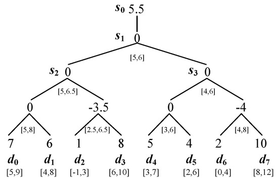
Figure 1. F-shift error tree T with error bound Δ = 2.

The F-shift transformation can be explained by the F-shift error tree T. For the error tree shown in Figure 1, we need to calculate the shift coefficient values of each node from bottom to up. First, for each leaf node $d_i$, we can use a data range $[{\underset{\_}{d}}_i,{\overline{d}}_i]$ to substitute the original data. The F-shift transformation needs to guarantee each $\left|d_i-{\widehat{d}}_i\right|\le \Delta$, where ${\widehat{d}}_i$ is the reconstructed data of $d_i$. Therefore, $[{\underset{\_}{d}}_i,{\overline{d}}_i]$ can be expressed as $\left[d_i-\Delta ,d_i+\Delta \right]$. Next, we need to determine which internal node coefficient needs to be retained. Let $innod{e}_j$ be the inner node, and $d_L$ and $d_{\mathrm{R}}$ be the left and right leaf nodes of $innod{e}_j$, respectively. Then, the corresponding data ranges of $d_L$ and $d_R$ are $[{\underset{\_}{d}}_L,{\overline{d}}_L]$ and $[{\underset{\_}{d}}_R,{\overline{d}}_R]$, respectively. The shift coefficient $s_j$ of $innod{e}_j$ can be obtained using the following:

Case 1: $[{\underset{\_}{d}}_L,{\overline{d}}_L]\cap [{\underset{\_}{d}}_R,{\overline{d}}_R]=\varphi$. This shows that the values of the two leaf nodes are quite different, and the shift coefficient $s_j$ of their parent node $innod{e}_j$ needs to be retained, which is:

$$s_j=\frac{({\underset{\_}{d}}_L+{\overline{d}}_L)-({\underset{\_}{d}}_R+{\overline{d}}_R)}{4},(0<j<n),$$

(1)

where n is the original data size. Then, the updated data range $\left[{\underset{\_}{d}}_j,{\overline{d}}_j\right]$ of $innod{e}_j$ should be stored temporarily. That is:

$${\underset{\_}{d}}_j=\max \{{\underset{\_}{d}}_L-s_j,{\underset{\_}{d}}_R+s_j\},$$

(2)

$${\overline{d}}_j=\min \{{\overline{d}}_L-s_j,{\overline{d}}_R+s_j\}.$$

(3)

Case 2: $[{\underset{\_}{d}}_L,{\overline{d}}_L]\cap [{\underset{\_}{d}}_R,{\overline{d}}_R]\ne \varphi$. This shows that the difference between the two leaf nodes is small and within the given error bound. Therefore, the shift coefficient $s_j$ of the parent node $innod{e}_j$ does not need to be retained and $s_j$ can be directly expressed by 0. Thus, within a given error bound, the number of internal nodes can be reduced to achieve data compression. However, the update data range $[{\underset{\_}{d}}_j,{\overline{d}}_j]$ of $innod{e}_j$ should be stored temporarily. That is:

$$[{\underset{\_}{d}}_j,{\overline{d}}_j]=[{\underset{\_}{d}}_L,{\overline{d}}_L]\cap [{\underset{\_}{d}}_R,{\overline{d}}_R].$$

(4)

We named this procedure the one-step F-shift transformation. According to the above steps, the shift coefficient (high-frequency component) and the data range (low-frequency component) of each parent node can be calculated. Then, the parent nodes of each layer of the error tree T can be regarded as leaf nodes such that the shift coefficients and the data ranges of each layer can be calculated iteratively using a one-step F-shift transformation. Lastly, the value of the root node can be given by any value of its child node’s data range. Usually, we take the average value of the data range. That is:

$$s_0=\frac{{\underset{\_}{d}}_L+{\overline{d}}_R}{2}.$$

(5)

As shown in Figure 1, a one-step F-shift transformation is performed on each leaf node to obtain a set of a low-frequency component and a high-frequency component: {[5,8],[2.5,6.5],[3,6],[4,8],0, −3.5,0,−4}. Next, the one-step F-shift transformation is repeated on the low-frequency component until one data range is left in the low-frequency component. Lastly, we usually select the average of the data range as the final approximation coefficient. Table 1 shows the shift coefficients of each level of the F-shift transformation.

Table 1. F-shift decomposition of a four-pixel image.

Resolution	Low-Frequency Component	High-Frequency Component
8	{[5,9], [4,8], [−1,3], [6,10],[3,7], [2,6], [0,4], [8,12]}	------
4	{[5,8], [2.5,6.5], [3,6], [4,8]}	{0,3.5,0,−4}
2	{[5,6.5], [4,6]}	{0,0}
1	{[5,6]}	{0}

After calculating the coefficient value of each node, a shift error tree is formed. The reconstruction value of each leaf node can be computed using:

$${\widehat{d}}_i^{(S)}={\displaystyle \sum _{s_j\in path(d_i)}{\delta }_{ij}}{s}_j,$$

(6)

where ${\widehat{d}}_i^{(S)}$ is the reconstructed data from the synopsis S. We set ${\delta }_{ij}=+1$ when $d_i$ is located on the left subtree of $s_j$ and set ${\delta }_{ij}=-1$ when $d_i$ is located on the right subtree of $s_j$. S is the set of shift coefficients. $path(d_i)$ is the node set that is located on the path from the root node to $d_i$ (not including $d_i$).

2.2. Two Dimensional F-Shift Transformation (TDFS)

The core of the TDFS [27] is to alternately do one-step F-shift transformations in each dimension. We can obtain the low-frequency and high-frequency components following a one-step F-shift transformation. Specifically, the TDFS first performs the a one-step F-shift transformation on each row. After that, we can get the low-frequency component, which is composed of the updated data range. Similarly, the same transformation should be performed on each column of the updated low-frequency component. The above steps of performing a one-step F-shift transformation to rows and columns, respectively, are called the first-level TDFS. Iteratively, the second-level TDFS, third-level TDFS, and so on, can be obtained until only one data range remains. Finally, we usually take the average of the last data range as the approximate value.

Figure 2 is an example of the TDFS. For the resolution of a $4\times 4$ image, we need to perform 2 levels of transformation to complete the TDFS. Figure 2a is the original data array, and $\Delta =2$. Figure 2b,c are the results of the first-level TDFS and the second-level TDFS, respectively. The shaded parts of the figures show the updated low-frequency component. Figure 2d is the final compression result. The shaded part is the approximate value.

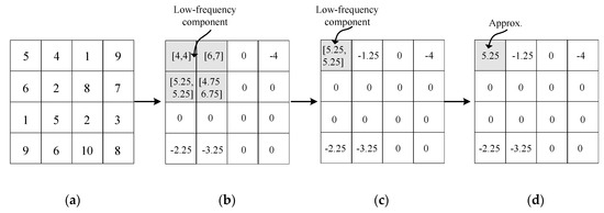
Figure 2. An example of a two–dimensional F-shift transformation (TDFS): (a) original data array, (b) first-level TDFS, (c) second-level TDFS, and (d) computing the approximation.

2.3. Contrast-Limited Adaptive Histogram Equalization (CLAHE)

The image histogram can show the pixel distribution of an image. By redistributing the distribution of the image histogram, the image contrast can be changed. Histogram equalization is actually a mapping transformation of the gray level of the original image, which can enlarge the dynamic range of the pixel gray value. Thus, the image contrast can be enhanced.

Suppose the grayscale range of an image is [0,n−1], with a gray level of $m$. Let $p_r(r)$ be the gray-level probability density function (PDF). Then, the probability of the kth gray level is [28]:

$$p_r(r_k)=\frac{n_k}{n},$$

(7)

where $k=0, 1, 2, \dots , m-1$ and $r_k$ stands for the kth grayscale. Then, the cumulative distribution function (CDF) $T(r_k)$ can be expressed as:

$$g=T(r_k)={\displaystyle \sum _{j=0}^k{p}_r(r_j)}={\displaystyle \sum _{j=0}^k\frac{n_j}{n}},$$

(8)

where $0\le g\le 1$.

Operating on the entire image as an image block is called global histogram equalization. Since the grayscale changes in different areas of a picture are different, if the global histogram is used, the local changes of the image will be ignored. The equalization of image regions is an adaptive histogram equalization (AHE) algorithm, which combines the advantages of global histogram equalization and considers the local contrast. This algorithm divides the image into several small regions first, then the CDF and image histogram are calculated from each small region, and finally, HE is performed on the pixels of each small region. Unfortunately, AHE tends to over-amplify noise in the relatively uniform regions of the image. To solve this problem, the CLAHE method was proposed. It has two main characteristics: on one hand, it is a method to limit the distribution of histograms to prevent excessive enhancement of noise points, while on the other hand, it uses interpolation to accelerate the histogram equalization. The steps of CLAHE [13] are:

(1) Split the input image into continuous and non-overlapping regions. The region size is generally set to $8\times 8$.

(2) Get the histogram of each region and use the threshold to clip the histogram. The CLAHE algorithm achieves the goal of limiting the magnification by clipping the histogram with a pre-defined threshold before calculating the CDF. This also limits the slope of the transformation function.

(3) Reallocate the pixel values, and distribute the clipped pixel values evenly below the histogram. Figure 3a,b are the histogram distribution before and after clipping, respectively.

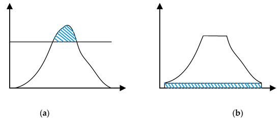
Figure 3. Histogram distribution: (a) before clipping and (b) after clipping.

(4) Perform a local histogram equalization on all regions.

(5) Use a linear interpolation for pixel value reconstruction. Suppose the gray value of the sample point P is s, and the new gray value after a linear interpolation is s’. The sample points of its surrounding regions are P₁, P₂, P₃, and P₄, and the gray-level mappings of s are $g_{P_1}(s)$, $g_{P_2}(s)$, $g_{P_3}(s)$, and $g_{P_4}(s)$, respectively. For the pixels in the corners, the new gray value is equal to the gray-level mapping of s of this region. For example:

$$s^{\prime }=g_{P_1}(s).$$

(9)

For the pixels on the edges, the new gray value is the interpolation of the gray-level mapping of s of the two samples of the surrounding regions. For example:

$$s^{\prime }=(1-\alpha )g_{P_1}(s)+\alpha g_{P_2}(s).$$

(10)

For the pixels of the center of the image, the new gray value is the interpolation of the gray-level mapping of s of the four samples of the surrounding regions. For example:

$$s^{\prime }=(1-\beta )((1-\alpha )g_{P_1}(s)+\alpha g_{P_2}(s))+\beta ((1-\alpha )g_{P_3}(s)+\alpha g_{P_4}(s)),$$

(11)

where α and β are the normalized distances with respect to the point P₁.

3. Proposed Method

Our smart image enhancement is performed in the process of image decompression. Therefore, image compression is a pre-required phase. The image compression method uses the TDFS [27], which is the two-dimensional F-shift transformation. In order to obtain a compromise between the compression effect and the image enhancement effect, we only performed the first-level TDFS on the image. The later compression uses a non-standard two-dimensional wavelet transform (NSTW) [4].

Figure 4 shows the image compression process we performed before the image enhancement. In this example, the error bound $\Delta$ was still set to 2. Figure 4a shows the original image pixels with a resolution of $4\times 4$. Figure 4b is the result obtained after performing the first-level TDFS on the original data. Figure 4c is the approximation values of the low-frequency component shown in Figure 4b. Here, the approximate value of each point was the average of the corresponding data range, which is shown in the shaded part of Figure 4c. Figure 4d is the result after performing NSTW on the approximate part of Figure 4c. It should be noted that when we performed the NSTW, the detailed coefficients were obtained by dividing 2, instead of dividing by $\sqrt{2}$. This was because we wanted to get coefficient values of the same order as the TDFS coefficients.

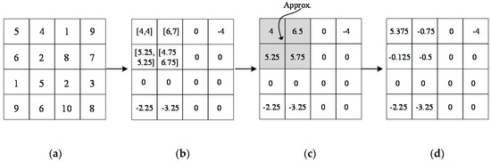
Figure 4. The compression process before the enhancement: (a) original data array, (b) first-level TDFS, (c) compute the approximation, and (d) non-standard two-dimensional wavelet transform (NSTW) for the approximation.

After obtaining the compressed data, the steps of our enhanced method were as follows:

Step 1. Adjust the first coefficient $s_{00}$ of the synopsis $S$ using the adaptive coefficient adjustment formula. Note that, as shown in Figure 4d, the wavelet synopsis S was a set of the non-zero values and the first coefficient $s_{00}$ was 5.375.

Step 2: Incompletely decompress the synopsis S and enhance the low-frequency component. Note that here we decompressed the synopsis to the second-to-last level rather than the final level.

Step 3: Complete the decompression and further enhancement. In this step, the synopsis was decompressed to the final level.

Figure 5 shows the flowchart of the proposed method.

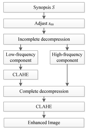
Figure 5. The steps of our enhancement method. CLAHE: Contrast-limited adaptive histogram equalization.

3.1. Adaptive Coefficient Adjustment

During the decompression, the first step was to adjust the image brightness to a suitable brightness such that the overall brightness of the image was not too bright or too dark. In our previous work [29], as well as in our current work, we carried out experiments on medical images and ordinary images. We first evaluated 120 images subjectively and divided them into three types: underexposed images, moderately exposed images, and overexposed images. Through the experiment, we found that when the cut-off values were 90 and 150, the classification accuracy was higher than 85 and 170 (that is, equally dividing 0 to 255 into three bins). Therefore, through experimental experience, we chose 90 and 150 as the cut-off points for an underexposed image and an overexposed image.

According to the properties of the previous compression scheme, the first coefficient of the wavelet synopsis essentially represents the mean of the gray value of the original image. Therefore, it is a representation of the image brightness. In this way, the image brightness can be adjusted through the first coefficient $s_{00}$. The adaptive coefficient adjustment equation is:

$$s_{00}^{\prime }=\lambda s_{00},$$

(12)

$$\lambda =\{\begin{array}{cc}1+\frac{90-s_{00}}{128},& 0\le s_{00}<90\\ 1,& 90\le s_{00}\le 150\\ 1-\frac{s_{00}-150}{128},& 150<s_{00}\le 255\end{array}$$

(13)

where $\lambda$ is the adjustment factor and $s_{00}^{\prime }$ is the updated approximation coefficient.

Remark 1: If the value of $s_{00}$ is changed, the image gray value will be affected when decompressed, e.g., given an increment $\mu$ to $s_{00}$, then each pixel will be increased by $\mu$.

From the data reconstruction Equation (6), we can see that $s_{00}$ has a global role in data reconstruction. The reconstruction of each pixel needs to add the value of $s_{00}$. Therefore, if we increase $s_{00}$ by $\mu$, then each pixel will be increased by $\mu$.

Remark 2: The transformation of the image gray value caused by the change of $s_{00}$ does not change the high-frequency components.

The change of $s_{00}$ only affects the reconstructed value of the original data, and the coefficients of the internal nodes of the error tree will not be affected. Therefore, the transformation of the image gray value caused by the change of $s_{00}$ does not change the high-frequency components.

3.2. Incomplete Decompression and Enhancing the Low-Frequency Component

Suppose the original image data size is $n\times n$, where $n=2^m$. Therefore, a complete compression of this image requires $m$ levels of transformation. After adjusting the first coefficient $s_{00}$, we need to decompress the image. To alleviate the blocking effect, we chose to enhance the decompressed synopsis when decompressing to a level of $m-1$ (the second-to-last level).

When the synopsis is decompressed to this level, the whole frame and main information of the image are contained in the low-frequency component. Then, CLAHE can be used to enhance the low-frequency component. This is the first time to use CLAHE to achieve the enhancement effect. Usually, the noise information exists in the high-frequency component; therefore, we kept the high-frequency component unchanged in this step to suppress the noise signal.

3.3. Complete Decompression and Further Enhancement

After the above steps, we will get the updated low-frequency component and the unchanged high-frequency component. At this point, only the last level of decompression is needed to get the decompressed image. After getting the reconstructed image, CLAHE is needed to enhance the image to make its detail more abundant.

4. Experimental Results

4.1. Impact of the Error Bound on the Enhancement and Compression Results

Figure 6, Figure 7 and Figure 8 show the enhanced images under different error bounds with $150<s_{00}\le 255$, $90\le s_{00}\le 150$, and $0\le s_{00}<90$. Theoretically, as the error bound increases, the high-frequency component will lose more and more detailed information. From the experimental results, we see that as the error bound increased, the brightness, contrast, and details of the image became weaker. For the images of Figure 6 and Figure 7, different error bounds had little effect on the image quality, while in the image of Figure 8, the image quality was very different and the margin was different. It can be seen from the results that for images with lower brightness, the enhancement effect was greatly affected by the error bound. In order to obtain a higher quality image, the error bound needed to be smaller.

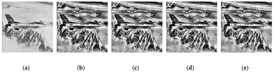
Figure 6. The enhanced image under different error bounds: (a) original image, (b) Δ = 0, (c) Δ = 2, (d) Δ = 5, and (e) Δ = 8.

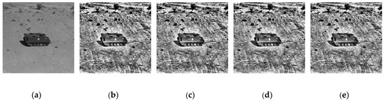
Figure 7. The enhanced image under different error bounds: (a) original image, (b) Δ = 0, (c) Δ = 2, (d) Δ = 5, and (e) Δ = 8.

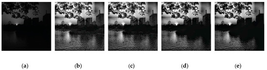
Figure 8. The enhanced image under different error bounds: (a) original image, (b) $\Delta =0$, (c) $\Delta =2$, (d) $\Delta =5$, and (e) $\Delta =8$.

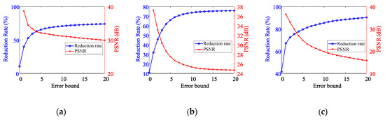
Figure 9 shows the trend of the compression effect and image quality under different error bounds in the images in Figure 6a, Figure 7a, and Figure 8a. The step of the error bound was 1. Here, the peak signal-to-noise ratio (PSNR) was used to evaluate the enhancement effect, and the data reduction rate was used to measure the compression effect. The reduction rate $r$ is defined as:

$$r=\frac{original\_data\_size-synopses\_size}{original\_data\_size},$$

(14)

where $synopses\_size$ represents the size of the synopsis $S$ obtained using our method and $original\_data\_size$ represents the size of the original image. We chose the enhanced image of $\Delta =0$ as a reference image for calculating the PSNR. The selection of this parametric setting was due to the loss of details being the least when $\Delta =0$. From Figure 9, we found that as the error bound increased, the PSNR of the image decreased and the reduction rate increased. We also found that images with a low brightness were more sensitive to the error bound. We found that a high compression effect and high image quality could not be achieved at the same time. Therefore, an appropriate error bound should be chosen to reach a compromise between the compression effect and image quality. In practical applications, this error bound is obtained through experience.

Figure 9. The trend of the image compression effect and image quality under different error bounds. (a) the result of Figure 6a, (b) the result of Figure 7a, and (c) the result of Figure 8a. PSNR: Peak signal-to-noise ratio.

4.2. Comparison of the Enhancement Effect of Different Methods

In this section, we compared our method with CLAHE [13] and CLAHE_DWT [25]. Figure 10, Figure 11, Figure 12, Figure 13, Figure 14 and Figure 15 show the images enhanced with different methods at different brightness levels. More concretely, Figure 10 and Figure 11 show the enhanced images with $150<s_{00}\le 255$, Figure 12 and Figure 13 show the enhanced images with $90\le s_{00}\le 150$, and Figure 14 and Figure 15 show the enhanced images with $0\le s_{00}<90$.

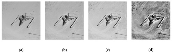
Figure 10. Comparison of the images enhanced using different methods: (a) original image, (b) CLAHE [13], (c) CLAHE_DWT [25], and (d) our method.

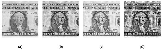
Figure 11. Comparison of the images enhanced using different methods: (a) original image, (b) CLAHE [13], (c) CLAHE_DWT [25], and (d) our method.

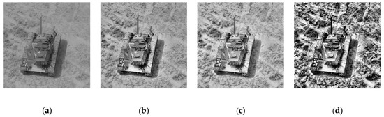
Figure 12. Comparison of the images enhanced using different methods: (a) original image, (b) CLAHE [13], (c) CLAHE_DWT [25], and (d) our method.

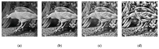
Figure 13. Comparison of the images enhanced using different methods: (a) original image, (b) CLAHE [13], (c) CLAHE_DWT [25], and (d) our method.

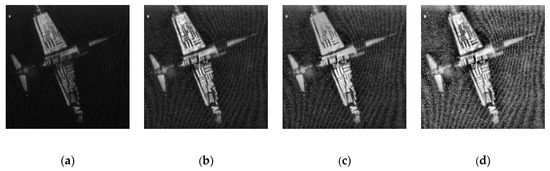
Figure 14. Comparison of the images enhanced using different methods: (a) original image, (b) CLAHE [13], (c) CLAHE_DWT [25], and (d) our method.

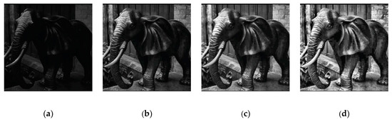
Figure 15. Comparison of the images enhanced using different methods: (a) original image, (b) CLAHE [13], (c) CLAHE_DWT [25], and (d) our method.

The error bound was set to 5, 5, 5, 5, 3, and 3 for Figure 10, Figure 11, Figure 12, Figure 13, Figure 14 and Figure 15, respectively. According to Figure 10, Figure 11, Figure 12, Figure 13, Figure 14 and Figure 15, we observed that the overall brightness of these images was greatly improved. It can be seen from the results that the image visual effects obtained using our method were better than CLAHE [13] and CLAHE_DWT [25], and the better visual effect was not only reflected in the image contrast but also in the image details.

Generally, there are two types of image quality evaluation methods: one is the full-reference image quality evaluation (e.g., PSNR, structural similarity index measurement (SSIM)), and the other is the non-reference image quality evaluation (e.g., mean, standard deviation (SD), entropy, average gradient (AG)). Because there was no ideal reference image, the non-reference image quality evaluation was more suitable for the comparison of image enhancement effects. Table 2 shows the mean [30,31], SD [30,32,33], entropy [31,32,34], and AG [31,32] of the images obtained using the above methods, which represent the average brightness, contrast, detail richness, and clarity of the image, respectively. The above evaluation parameters can be obtained using the following formula:

$$\mathrm{Mean}=\frac{1}{m\times n}{\displaystyle \sum _{i=0}^{m-1}{\displaystyle \sum _{j=0}^{n-1}{d}_{ij}}},$$

(15)

$$\mathrm{SD}=\sqrt{\frac{1}{m\times n-1}{{\displaystyle \sum _{i=0}^{m-1}{\displaystyle \sum _{j=0}^{n-1}\left|d_{ij}-\mathrm{Mean}\right|}}}^2},$$

(16)

$$\mathrm{Entropy}=-{\displaystyle \sum _{k=0}^{255}p(k)\times {\log }_{2}p(k)},$$

(17)

$$\mathrm{AG}=\frac{1}{m\times n}{\displaystyle \sum _{i=0}^{m-1}{\displaystyle \sum _{j=0}^{n-1}\sqrt{\frac{{({\nabla }_i)}^2+{({\nabla }_j)}^2}{2}}}},$$

(18)

where Mean is the mean of the image. $m$ is the number of rows and $n$ is the number of columns. $d_{ij}$ is the gray value of each pixel. SD is the standard deviation of the image. Entropy is the entropy of the image. $p(k)$ stands for the kth gray level probability. ${\nabla }_i$ and ${\nabla }_j$ stand for the gradient of the horizontal and vertical direction, where ${\nabla }_i=d_{ij}-d_{(i-1)j}$ and ${\nabla }_j=d_{ij}-d_{i(j-1)}$, and i and j are the row and the column numbers.

Table 2. Comparison of the evaluation parameters of different methods.

Images	Methods	Mean	SD	Entropy	AG
Figure 10	Original	175.33	22.12	4.00	2.32
	CLAHE [13]	177.31	24.00	5.73	3.66
	CLAHE_DWT [25]	174.04	25.08	5.74	3.36
	Our method	145.53	38.75	7.23	10.42
Figure 11	Original	172.16	55.83	6.98	15.25
	CLAHE [13]	156.15	67.02	7.71	21.90
	CLAHE_DWT [25]	161.73	69.02	7.32	18.99
	Our method	134.30	71.25	7.95	22.90
Figure 12	Original	132.38	27.06	5.50	5.00
	CLAHE [13]	145.48	39.08	7.16	10.15
	CLAHE_DWT [25]	165.83	49.75	7.53	12.25
	Our method	131.32	70.14	7.98	20.10
Figure 13	Original	95.39	53.78	6.12	7.01
	CLAHE [13]	107.27	59.31	7.76	9.79
	CLAHE_DWT [25]	127.63	67.71	7.95	12.38
	Our method	125.44	71.51	7.99	14.92
Figure 14	Original	32.52	25.11	5.43	2.55
	CLAHE [13]	55.16	39.74	6.52	7.12
	CLAHE_DWT [25]	94.57	53.48	7.02	8.68
	Our method	93.92	48.86	7.48	12.95
Figure 15	Original	20.12	19.68	5.63	1.67
	CLAHE [13]	51.67	42.00	6.95	4.40
	CLAHE_DWT [25]	75.26	55.24	7.39	5.61
	Our method	92.60	61.72	7.72	7.90

In Table 2, the image brightness can be altered to a suitable range based on our method. We show the best results in bold, and the best value of Mean is the maximum value in the range of [90, 150]. In most cases, the SD, entropy, and AG of the algorithm are greater than the other two algorithms and the original image, which was consistent with our subjective feelings. Therefore, both subjective and objective results show that our algorithm can get better image contrasts and more image details. In addition, our algorithm can also achieve data compression. Through calculations for the images in Figure 10, Figure 11, Figure 12, Figure 13, Figure 14 and Figure 15, the reduction rates were 76.47%, 43.19%, 55.88%, 59.73%, 71.95%, and 75.03%, respectively.

4.3. Method Validation

To further prove the effectiveness of our method, we propose several schemes to verify it.

Scheme 1: This scheme can be simply described as $s_{00}$ adjustment plus CLAHE for the low-frequency component.

Specifically, during the decompression process, $s_{00}$ is adjusted adaptively; then, the synopsis is decompressed to the second-to-last level. After performing CLAHE for the decompressed low-frequency component, the synopsis is decompressed completely and the final enhanced image is obtained.

Scheme 2: This scheme can be simply described as $s_{00}$ adjustment plus CLAHE for a completely decompressed image.

Specifically, during the decompression process, $s_{00}$ is adjusted adaptively; then, the synopsis is decompressed completely and the final enhanced image is obtained by using CLAHE for the decompressed image.

Scheme 3: This scheme can be simply described as two-stage CLAHE for the original image.

Specifically, one CLAHE enhancement is used after another CLAHE enhancement of the original image.

Scheme 4: This scheme can be simply described as $s_{00}$ adjustment plus two-stage CLAHE for the low-frequency component.

Specifically, during the decompression process, $s_{00}$ is adjusted adaptively; then, the synopsis is decompressed to the second-to-last level. After that, a two-stage CLAHE enhancement is used for the low-frequency component. Lastly, the enhanced image is obtained using the complete decompression.

Scheme 5: This scheme can be simply described as $s_{00}$ adjustment plus two-stage CLAHE for a complete decompressed image.

Specifically, during the decompression process, $s_{00}$ is adjusted adaptively; then, the synopsis is decompressed completely. After that, a two-stage CLAHE enhancement is used for the complete decompressed image. Finally, the enhanced image can be obtained.

Our method: Our method can be simply described as $s_{00}$ adjustment plus CLAHE for the low-frequency component plus CLAHE for the complete decompressed image.

That is, during the decompression process, $s_{00}$ is adjusted adaptively; then, the synopsis is decompressed to the second-to-last level. After the CLAHE enhancement for the decompressed low-frequency component, the synopsis is decompressed completely. Finally, the CLAHE enhancement is used again for the complete decompressed image and the enhanced image can be obtained.

Figure 16, Figure 17, Figure 18 and Figure 19 are comparisons between the above schemes and our method. From the experimental results of schemes 1 and 2, we found that compared with the scheme of using CLAHE directly on the original image, the $s_{00}$ adjustment and CLAHE during the decompression play positive roles in the image enhancement. From the results of schemes 3–5 and our method, we found that using CLAHE twice can get a better enhancement effect than schemes 1–2 and CLAHE. For the schemes using CLAHE twice, we found that the image enhancement effect obtained using our method was the best. For scheme 4, using CLAHE twice to enhance the low-frequency component may reduce the effect of the high-frequency component, which makes the reconstructed image not clear enough. For scheme 5, using CLAHE twice for the decompressed image could not effectively utilize the advantages of separately processing the low-frequency and high-frequency components. This was because the low-frequency component usually has very large information entropy, while the high-frequency component usually has a smaller information entropy. Excessive enhancement of the low-frequency component or too little enhancement will reduce the enhancement effect. Table 3 shows the objective evaluation indicators of the comparison schemes. The best results are shown in bold. It can be seen from Table 3 that our method can achieve the best results on more indicators than other schemes. Those objective indicators also conformed to our subjective feelings. Therefore, our method demonstrated its advantages both subjectively and objectively.

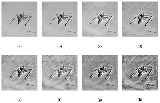
Figure 16. Comparison results of different schemes: (a) original image, (b) CLAHE, (c) scheme 1, (d) scheme 2, (e) scheme 3, (f) scheme 4, (g) scheme 5, and (h) our method.

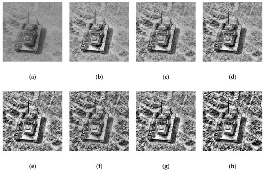
Figure 17. Comparison results of different schemes: (a) original image, (b) CLAHE, (c) scheme 1, (d) scheme 2, (e) scheme 3, (f) scheme 4, (g) scheme 5, and (h) our method.

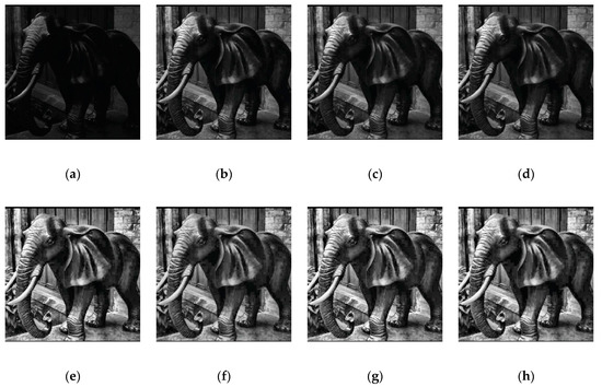
Figure 18. Comparison results of different schemes: (a) original image, (b) CLAHE, (c) scheme 1, (d) scheme 2, (e) scheme 3, (f) scheme 4, (g) scheme 5, and (h) our method.

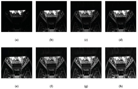
Figure 19. Comparison results of different schemes: (a) original image, (b) CLAHE, (c) scheme 1, (d) scheme 2, (e) scheme 3, (f) scheme 4, (g) scheme 5, and (h) our method.

Table 3. Comparison of evaluation parameters of different methods.

Images	Methods	Mean	SD	Entropy	AG
Figure 16	Original	175.33	22.12	4.00	2.32
	CLAHE [13]	177.31	24.00	5.73	3.66
	Scheme 1	146.86	25.65	6.18	4.44
	Scheme 2	147.15	22.85	5.81	3.68
	Scheme 3	167.66	32.51	6.72	8.64
	Scheme 4	145.00	40.17	7.29	10.84
	Scheme 5	145.73	31.82	6.79	8.92
	Our method	141.50	40.67	7.34	11.60
Figure 17	Original	132.38	27.06	5.50	5.00
	CLAHE [13]	145.48	39.08	7.16	10.15
	Scheme 1	143.29	45.90	7.48	11.05
	Scheme 2	140.98	46.34	7.51	13.70
	Scheme 3	136.79	63.18	7.91	20.96
	Scheme 4	132.65	69.80	7.97	19.77
	Scheme 5	130.49	70.87	7.98	24.66
	Our method	130.35	70.88	7.99	20.52
Figure 18	Original	20.12	19.68	5.63	1.65
	CLAHE [13]	51.67	42.00	6.95	4.39
	Scheme 1	57.31	40.57	6.91	4.09
	Scheme 2	57.70	40.72	6.92	4.24
	Scheme 3	91.16	62.22	7.74	7.98
	Scheme 4	94.04	61.13	7.73	7.94
	Scheme 5	94.10	61.05	7.73	8.17
	Our method	93.67	60.88	7.74	8.32
Figure 19	Original	14.07	39.75	4.13	2.28
	CLAHE [13]	29.25	47.36	5.20	4.43
	Scheme 1	33.52	47.21	4.91	3.90
	Scheme 2	33.85	46.75	5.13	4.15
	Scheme 3	45.20	55.36	6.24	5.83
	Scheme 4	47.63	56.94	6.12	6.00
	Scheme 5	48.04	55.58	6.29	6.30
	Our method	48.24	57.09	6.35	6.10

5. Conclusions

In this study, we developed a smart image enhancement method during decompression and designed a variety of schemes to verify the effectiveness of our method. We obtained the compressed data by using the first-level TDFS and NSTW for the original image. During decompression, the overall brightness of the image was adaptively adjusted using the first coefficient $s_{00}$. To improve the image contrast and enrich the image details, we implemented the CLAHE enhancement for the low-frequency component and reconstructed images during decompression. The results showed that this enhancement strategy could effectively utilize the advantages of separately processing the low-frequency and high-frequency components and balance the enhancement effect. The experimental results showed that compared with the methods of CLAHE [13] and CLAHE_DWT [25], our scheme could further improve the image contrast while making the image details more abundant. The proposed methods provided in this paper further extend our previous work [26], and a comprehensive model was suggested for smart image enhancement. This smart image enhancement method can be further applied to intelligent image processing applications, such as face recognition and smart system inspection. Our future work will focus on applying the above-mentioned smart image enhancement method to smart city surveillance and rapid responses to potential pandemic outbreaks.

References

- Hsia, C.H.; Yang, J.H.; Chiang, J.S. Complexity reduction method for ultrasound imaging enhancement in tetrolet transform domain. J. Supercomput. 2020, 76, 1438–1449. [Google Scholar] [CrossRef]
- Xia, K.J.; Wang, J.Q.; Cai, J. A novel medical image enhancement algorithm based on improvement correction strategy in wavelet transform domain. Cluster Comput. 2019, 22, 10969–10977. [Google Scholar] [CrossRef]
- Pang, C.; Zhang, Q.; Zhou, X.; Hansen, D.; Wang, S.; Maeder, A. Computing unrestricted synopses under maximum error bound. Algorithmica 2013, 65, 1–42. [Google Scholar] [CrossRef]
- Zhang, Q.; Pang, C.; Hansen, D. On multidimensional wavelet synopses for maximum error bounds. In International Conference on Database Systems for Advanced Applications; Springer: Berlin/Heidelberg, Germany, 2009; pp. 646–661. [Google Scholar]
- Rahman, S.; Rahman, M.M.; Abdullah-Al-Wadud, M.; Al-Quaderi, G.D.; Shoyaib, M. An adaptive gamma correction for image enhancement. EURASIP J. Image Video Process. 2016, 1, 1–13. [Google Scholar] [CrossRef]
- Lim, S.H.; Isa, N.A.M.; Ooi, C.H.; Vin Toh, K.K. A new histogram equalization method for digital image enhancement and brightness preservation. Signal Image Video Process. 2015, 9, 675–689. [Google Scholar] [CrossRef]
- Zhuang, L.; Guan, Y. Image enhancement via subimage histogram equalization based on mean and variance. Comput. Intell. Neurosci. 2017, 1–12. [Google Scholar] [CrossRef] [PubMed]
- Arora, S.; Agarwal, M.; Kumar, V.; Gupta, D. Comparative study of image enhancement techniques using histogram equalization on degraded images. Int. J. Eng. Technol. 2018, 7, 468–471. [Google Scholar] [CrossRef]
- Rahman, Z.U.; Jobson, D.J.; Woodell, G.A. Retinex processing for automatic image enhancement. J. Electron. Imaging. 2004, 13, 100–110. [Google Scholar]
- Lee, S. An efficient content-based image enhancement in the compressed domain using retinex theory. IEEE Trans. Circuits Syst. Video Technol. 2007, 17, 199–213. [Google Scholar] [CrossRef]
- Anand, S.; Gayathri, S. Mammogram image enhancement by two-stage adaptive histogram equalization. Optik 2015, 126, 3150–3152. [Google Scholar] [CrossRef]
- Sargun, S.; Rana, S.B. Performance evaluation of HE, AHE and fuzzy image enhancement. Int. J. Comput. Appl. 2015, 122, 14–19. [Google Scholar] [CrossRef]
- Zuiderveld, K. Contrast limited adaptive histogram equalization. Graph. Gems 1994, 474–485. [Google Scholar]
- Singh, P.; Mukundan, R.; Ryke, R.D. Feature enhancement in medical ultrasound videos using contrast-limited adaptive histogram equalization. J. Digital Imaging 2019, 1–13. [Google Scholar] [CrossRef]
- Wang, J.W.; Le, N.T.; Lee, J.S.; Wang, C.C. Color face image enhancement using adaptive singular value decomposition in fourier domain for face recognition. Pattern Recognit. 2016, 57, 31–49. [Google Scholar] [CrossRef]
- Makandar, A.; Halalli, B. Image enhancement techniques using highpass and lowpass filters. Int. J. Comput. Appl. 2015, 109, 21–27. [Google Scholar] [CrossRef]
- Kuo, C.M.; Yang, N.C.; Liu, C.S.; Tseng, P.Y.; Chang, C.K. An effective and flexible image enhancement algorithm in compressed domain. Multimed. Tools Appl. 2016, 75, 1177–1200. [Google Scholar] [CrossRef]
- Sharma, A.; Khunteta, A. Satellite image enhancement using discrete wavelet transform, singular value decomposition and its noise performance analysis. In Proceedings of the 2016 International Conference on Micro-Electronics and Telecommunication Engineering (ICMETE), Ghaziabad, India, 22–23 September 2016; pp. 594–599. [Google Scholar]
- Hsieh, C.T.; Lai, E.; Wang, Y.C. An effective algorithm for fingerprint image enhancement based on wavelet transform. Pattern Recognit. 2003, 36, 303–312. [Google Scholar] [CrossRef]
- Kim, S.; Kang, W.; Lee, E.; Paik, J. Wavelet-domain color image enhancement using filtered directional bases and frequency-adaptive shrinkage. IEEE Trans. Consum. Electron. 2010, 56, 1063–1070. [Google Scholar] [CrossRef]
- Uhring, W.; Jung, M.; Summ, P. Image processing provides low-frequency jitter correction for synchroscan streak camera temporal resolution enhancement. Opt. Metrol. Prod. Eng. 2004, 5457, 245–252. [Google Scholar]
- Yang, J.; Wang, Y.; Xu, W.; Dai, Q. Image and video denoising using adaptive dual-tree discrete wavelet packets. IEEE Trans. Circuits Syst. Video Technol. 2009, 19, 642–655. [Google Scholar] [CrossRef]
- Shahane, P.R.; Mule, S.B.; Ganorkar, S.R. Color image enhancement using discrete wavelet transform. Digital Image Process. 2012, 4, 1–5. [Google Scholar]
- Zhang, C.; Ma, L.N.; Jing, L.N. Mixed frequency domain and spatial of enhancement algorithm for infrared image. In Proceedings of the 2012 9th International Conference on Fuzzy Systems and Knowledge Discovery, Sichuan, China, 29–31 May 2012; pp. 2706–2710. [Google Scholar]
- Huang, L.; Zhao, W.; Wang, J.; Sun, Z. Combination of contrast limited adaptive histogram equalisation and discrete wavelet transform for image enhancement. IET Image Process. 2015, 9, 908–915. [Google Scholar]
- Fan, R.; Li, X.; Zhao, H.; Zhang, H.; Pang, C.; Wang, J. Image enhancement method in decompression based on F-shift transformation. In Communications in Computer and Information Science, Proceedings of the 6th International Conference, ICDS 2019, Ningbo, China, 15–20 May 2019; Springer: Berlin/Heidelberg, Germany, 2020; Volume 1179, pp. 232–241. [Google Scholar]
- Li, X.; Fan, R.; Zhang, H.; Li, T.; Pang, C. Two-dimensional wavelet synopses with maximum error bound and its application in parallel compression. J. Intell. Fuzzy Syst. 2019, 37, 3499–3511. [Google Scholar] [CrossRef]
- Abdullah-Al-Wadud, M.; Kabir, M.H.; Dewan, M.A.A.; Chae, O. A dynamic histogram equalization for image contrast enhancement. IEEE Trans. Consum. Electron. 2007, 53, 593–600. [Google Scholar] [CrossRef]
- Li, X.; Li, T.; Zhao, H.; Dou, Y.; Pang, C. Medical image enhancement in F-shift transformation domain. Health Inf. Sci. Syst. 2019, 7, 1–8. [Google Scholar] [CrossRef]
- Lee, H.S.; Moon, S.W.; Eom, I.K. Underwater image enhancement using successive color correction and superpixel dark channel prior. Symmetry 2020, 12, 1220. [Google Scholar] [CrossRef]
- Li, B.; Xie, W. Image denoising and enhancement based on adaptive fractional calculus of small probability strategy. Neurocomputing 2016, 175, 704–714. [Google Scholar] [CrossRef]
- Qu, Z.; Xing, Y.; Song, Y. Image enhancement based on pulse coupled neural network in the nonsubsample shearlet transform domain. Math. Prob. Eng. 2019, 2019, 1–11. [Google Scholar] [CrossRef]
- Chang, D.C.; Wu, W.R. Image contrast enhancement based on a Histogram transformation of local standard deviation. IEEE Trans. Med. Imaging 1998, 17, 518–531. [Google Scholar] [CrossRef]
- Zhuang, L.; Guan, Y. Adaptive Image enhancement using entropy-based subhistogram equalization. Comput. Intell. Neurosci. 2018. [Google Scholar] [CrossRef]
© 2020 by the authors. Licensee MDPI, Basel, Switzerland. This article is an open access article distributed under the terms and conditions of the Creative Commons Attribution (CC BY) license (http://creativecommons.org/licenses/by/4.0/).