FPGA-Based Architecture for Sensing Power Consumption on Parabolic and Trapezoidal Motion Profiles

Abstract

The objective of this work is to design and implement a scalable Field-Programmable Gate Array (FPGA)-based motion control system for DC servo motors using a parabolic velocity profile for industrial applications. The implementation in this device allows the obtaining of a fast, flexible and low-cost system. The system is divided into control, communication and closed-loop coupling. The work also addresses a comparative analysis of the most used profiles, the trapezoidal and parabolic. The comparison is made considering the energy consumption of both profiles. As a consequence of the comparison made, the velocity profile can be selected to reduce production costs by saving energy and reducing wear on machinery. The discrete models of the velocity profiles are obtained through numerical methods that permit the control blocks to be implemented in an FPGA. To reduce maintenance costs and energy consumption in servo mechanisms, the derivation of the acceleration or jerk of the motor is shown. A Graphic User Interface (GUI) is presented, which allows monitoring the position, velocity and angular acceleration of the motor shaft. In addition, the developed interface supports modification of parameters of the final position and maximum velocity in the motor. The delivered current is compared, evaluating its decrease using a parabolic velocity profile. Finally, the experimental results are illustrated.

1. Introduction

Motors are used in a wide variety of applications, from washing machine [1] in homes to electric vehicles [2] in the transport sector. Modern control systems generally require more efficient techniques to execute the instructions at high velocity and get more accurate results. According to [3], the best way to achieve high performance in servo control is to remove the servo control loop implemented in a Digital Signal Processor (DSP) or in a microcontroller and transfer it to a high-velocity control loop in an Field-Programmable Gate Array (FPGA). The statement takes into account the advantages of using the FPGA as a controller. For example, FPGAs are flexible devices that have the ability of reconfigurable parallel processing [4,5] and, it is precisely the aforementioned aspect that allows the realization of a system of logical operations in parallel, which considerably reduces the computation time [6]. Finally, the FPGA has a comparatively simpler design cycle to be managed and requires less manual intervention [7,8].

FPGAs have established as a competitive option for the control of processes that require high-processing velocity. Examples of certain applications carried out with FPGA can be found in the literature [9,10,11,12]. In specific applications that use servo motors, lower cost of FPGA hardware is required to reduce the price of the system [13]. The use of an FPGA enables a greater scale of control loop integration, which is one of the premises of the modern industry. In this sense, achieving a high-level integration and density of the used Printed Circuit Board (PCB) for the control implementation is defined as one of the most important criteria in the sector [14]. The authors in [15] discuss the block architecture and strategy that must be implemented in the FPGA to connect a speed profile to a controller.

Currently, position control loops on motors employ a design that allows tracking of a reference. These designs, also called velocity profiles, are presented as piece wise finite order polynomials [16] and they play an important role in motion control applications. The main advantage of using velocity profiles is the reduction of vibrations and energy consumption [17]. The most used profiles are: trapezoidal [18] and parabolic [19]. The use of the mentioned velocity profiles is not limited to the control of electric motors but is applied in a wide range of applications [20,21]. This type of polynomial has essential parameters: velocity, acceleration, distance, trajectory to follow and the time of the route. The relationship between distance and time allows establishing other concepts such as jerk (derived from acceleration) [22].

According to [23], the planning of trajectories in machines and robots with multiple actuators began with the design of mechanical cams capable of generating the desired movements. The movements were synchronized with the mechanical couplings. Presently, trajectory planning is committed to the design of electronic cameras that allow servo-assisted mechanisms to be controlled in a more flexible way and where synchronization is completely achieved with software tools [24]. Therefore, it is possible to avoid repetitive design and manufacture of mechanical cams for each type of trajectory. On the other hand, movement is simplified by focusing solely on the control of the electric motor to generate different movement profiles.

Generally, position control in electric motors combines a position controller and a velocity profile generator. Heo et al. in [25] present a trapezoidal velocity profile generator and a position P-PI controller to produce a trajectory from a reference. The trapezoidal profile causes a certain level of stress in the motors. Some research develops smoother profiles to avoid affecting the motor function. For example, [26] presents a curve velocity profile S to eliminate the aforementioned disadvantages. The authors in [27] shows an optimized S-curve model that reduces positioning time. The main advantage of the work is the proposal of a robust model.

In certain industrial applications, energy consumption is not considered to be a key element for the selection of profiles. This aspect represents an increase in production costs and pollution levels that the industrial sector generates, because it is precisely electric motors that represent the highest percentage of energy consumption. According to [28], the electricity consumption for electric motors up to 0.75 kW represents 9% of the total, between 0.75 kW and 375 kW is 68% and the rest 23%. This work presents a use case for DC motors with a power consumption up to 0.75 kW. However, it can be scaled to higher power motors. Currently, the reduction of energy consumption is an urgent need and the participation of the industry is essential [29]. Precisely, to advance in this regard, in 2012, the Energy Efficiency Directives of the European Union were approved. These directives establish a way forward to achieve greater energy efficiency [30].

Although smoother profiles have been developed, such as the S-curve velocity profile, it has been shown that flexibility in the trapezoidal and parabolic profile can be achieved with the proper selection of its parameters [31]. For this reason, the aforementioned profiles constitute the focus of this investigation.

Table 1. General comparison of the velocity profiles.

	Trapezoidal Velocity Profile	Parabolic Velocity Profile	S Velocity Profile
Advantage	This profile can be executed in shorter periods of time when using point-to-point movement	Parabolic profile reduces mechanical jerks	The profile makes the jerk constant for several periods of time, avoiding that the jerk goes to the infinite.
Limiting	Trapezoidal profile can produce undesirable mechanical jerks	Requires a longer cycle time	S profile is slower than the trapezoidal and parabolic profile.

shows a brief comparison of the main characteristics of the velocity profiles treated at work. Although the S profile is not addressed in the present investigation, its inclusion in the previous table was considered important. Furthermore,

Table 2. Summary of the state of the art.

Ref./Year	Implementation	Contributions
[16]/2017	Raspberry Pi 3 and FPGA ZYBO	The paper presents a comparison between the trapezoidal and s-curve velocity profile used in robotics and CNC machinery.
[25]/2019	TMS320C28346 microcontroller	A trapezoidal profile generator based on a cascaded P-PI position controller is proposed.
[32]/2008	MDi MC4000 Pro controller card	The model of polynomial s-curve motion profiles is generalized in a recursive form.
[33]/2013	TMS320F28335 controller	The position reference in consideration of jerk is generated in the control system of permanent magnet synchronous motor.
[34]/2019	PCI-7345	Tuning parameters are adjusted to place the zeros of the motion profile at a vibrating pole in the system to minimize vibration.
[35]/2007	PMDi MC4000 Pro controller card	Experimental results show the effectiveness and promising application ability of the algorithms in s-curve motion profiling.

presents a summary of similar works.

It is important to mention that greater efficiency in production chains is not the only justification for the development of this research. In addition, a correct modulation must be made in the maximum velocity of the actuators, since it allows the prevention of collisions or overheating in moving parts. The regulation of energy consumption directly affects production costs and it is precisely this characteristic that highlights the parabolic profile versus the trapezoidal profile, reducing the rate of change in acceleration with respect to time. The objective of the work is the practical FPGA-based implementation of a control for servo motors for industrial use, in addition to establishing a comparative analysis that results in the selection of the most suitable profile for the application. For this, a separate implementation of each module is carried out. The paper is structured as follows. Section 2 presents the analytical model of velocity profiles. In Section 3, the development and implementation of the modules that make up the motion control system is documented. The experimental results and the comparative analysis of the trapezoidal and parabolic profiles are presented in Section 4. A list of the acronyms used in this paper is presented at the end of the document and in the

Table A3. Relevant sign diagram.

Pin	Signal	Type	Description
4,6,7,8	M4-M1	Input	DAC digital inputs.
10	BRAKE	Input	Driver logical brake.
11	DIRECTION	Input	Sets the direction of rotation of the motor (1 -> Schedule).
14	${DAC}_{REF}$	Input	Take the reference voltage of the DAC in a range of 0 V to 5 V.
9	VCC	Input	Supply of the power that will move the motor.
1	OUT1	Output	Exit node of the first half of the H bridge.
15	OUT2	Output	Exit node of the second half of the H bridge.
13	CS OUT	Output	Current sensor amplifier output.

is shown the main signals used in the diagrams.

2. Analytical Model of Velocity Profiles

The trajectories are expressed as parametric functions of time and their analysis begins with the proposal of different velocity curves. First, the behavior of a parabolic velocity profile is analyzed, given by a function of the second degree and concludes with the study of the trapezoidal profile consisting of a sectioned function of the first degree.

2.1. Parabolic Velocity Profile

A parabolic trajectory belongs to a quadratic function and in turn, the derivative of said function is a line of first grade, as shown in Figure 1a. The equation that describes the acceleration line is defined in Equation (1).

$$\alpha \left(t\right)=\frac{-2a}{T}t+a$$

(1)

where: T is the sample time, a is the acceleration value and t is the time.

The angular velocity shown in Equation (2) and illustrated in Figure 1b is obtained by integrating Equation (1) from 0 to T.

$$\omega \left(t\right)={\int }_0^T\alpha \left(t\right)dt+\omega \left(0\right)$$

(2)

Equation (3) is obtained by solving the integral. The maximum value is presented at the point where the acceleration line intersects the abscissa axis. For this reason, to evaluate this function in $\frac{T}{2}$ the maximum velocity is obtained as Equation (4). Finally, the angular position function is calculated as in Equation (5).

$$\omega \left(t\right)=\frac{-a{t}^2}{T}+at,\omega \left(0\right)=0$$

(3)

$${\omega }_{max}=\omega (T/2)$$

(4)

$$\theta \left(t\right)=\frac{-a{t}^3}{3T}+\frac{a{t}^2}{2},\theta \left(0\right)=0$$

(5)

Figure 1c shows the result of evaluating the previously calculated position function from 0 to T.

The final position is obtained by evaluating $\theta \left(t\right)$ in T:

$${\theta }_f=\frac{2a{T}^2}{12}$$

(6)

For application purposes it is convenient to define Equation (7) in terms of the maximum velocity:

$${\theta }_f=\frac{2T}{3}{\omega }_{max}$$

(7)

$$a=\frac{4{\omega }_{max}}{T}$$

(8)

$$T=\frac{3{\theta }_f}{2{\omega }_{max}}$$

(9)

The development of these equations allows the conclusion that the desired position and the maximum acceleration depend solely on the end position assigned by the user and the maximum velocity of the motor. In the implementation of the parabolic profile (in its digital form), the values T, a and $m=\frac{-2a}{T}$ are used as coefficients to iteratively calculate the different positions for each instant of time through of numerical integration.

2.2. Trapezoidal Velocity Profile

The trapezoidal velocity profile is described as a sectioned function in two straight lines that have a slope and a line parallel to the X axis. The function that represents the acceleration of this profile is also given by a sectioned function in constant values as shown in Figure 2a, but they could be modified and experimented with different geometries of the trapezoid.

The functions that describe the velocity and position of the trapezoidal profile require integration by parts in the time interval established in the acceleration function.

$$\alpha \left(t\right)=\left\{\begin{array}{c}a0\le t\le \frac{T}{3},\hfill \\ 0\frac{T}{3}\le t\le \frac{2T}{3},\hfill \\ -a\frac{2T}{3}\le t<T.\hfill \end{array}\right.$$

(10)

Table 3. Angular velocity for each acceleration interval.

Interval	$\mathit{\alpha }\left(\mathit{t}\right)$	Function	$\mathit{\omega }\left(\mathit{t}\right)$
$0<t\le \frac{T}{3}$	a	$\omega \left(t\right)={\int }_0^{\frac{T}{3}}\alpha \left(t\right)dt+\omega \left(0\right)$	$\omega \left(t\right)=at,\omega \left(0\right)=0$
$\frac{T}{3}<t\le \frac{2T}{3}$	0	$\omega \left(t\right)={\int }_{\frac{T}{3}}^{\frac{2T}{3}}\alpha \left(t\right)dt+\omega \left(\frac{T}{3}\right)$	$\omega \left(t\right)=\frac{aT}{3}$
$\frac{2T}{3}<t\le T$	−a	$\omega \left(t\right)={\int }_{\frac{2T}{3}}^T\alpha \left(t\right)dt+\omega \left(\frac{2T}{3}\right)$	$\omega \left(t\right)=-at+aT$

summarizes the results obtained from angular velocity after solving each integral. The maximum velocity of the motor is represented by Equation (11), which results from evaluating the first result in $\frac{T}{3}$. Figure 2b presents the velocity graph obtained.

$${\omega }_{max}=\frac{aT}{3}$$

(11)

Obtaining the angular position function requires the same part integration procedure used for the velocity function.

Table 4. Position for each acceleration interval.

Interval	$\mathit{\alpha }\left(\mathit{t}\right)$	Function	$\mathit{\theta }\left(\mathit{t}\right)$
$0<t\le \frac{T}{3}$	a	$\theta \left(t\right)={\int }_0^{\frac{T}{3}}\omega \left(t\right)dt+\theta \left(0\right)$	$\theta \left(t\right)=\frac{a{t}^2}{2},\theta \left(0\right)=0$
$\frac{T}{3}<t\le \frac{2T}{3}$	0	$\theta \left(t\right)={\int }_{\frac{T}{3}}^{\frac{2T}{3}}\omega \left(t\right)dt+\theta \left(\frac{T}{3}\right)$	$\theta \left(t\right)=\frac{aT}{3}t-\frac{a{T}^2}{18}$
$\frac{2T}{3}<t\le T$	−a	$\theta \left(t\right)={\int }_{\frac{2T}{3}}^T\omega \left(s\right)dt+\theta \left(\frac{2T}{3}\right)$	$\theta \left(t\right)=-\frac{a{t}^2}{2}t+atT-\frac{5a{T}^2}{18}$

summarizes the results of evaluating the integral for each of the time intervals. From the values presented, Figure 2c is presented.

The final position is obtained by evaluating $\theta \left(t\right)$ in T in Equation (12) and Equation (13) is obtained.

$${\theta }_f=\theta \left(T\right)$$

(12)

$${\theta }_f=\frac{2a{T}^2}{9}$$

(13)

It is convenient to factor the Expression (14) into the product of $\frac{aT}{3}$ by $\frac{2T}{3}$ in order to substitute with Equation (11) and describe the final position in terms of maximum velocity and time period.

$${\theta }_f=\frac{2T}{3}{\omega }_{max}$$

(14)

From the previous equation can be solved T and taking into account Equation (15), the acceleration constant is solved in Equation (16).

$$T=\frac{3{\theta }_f}{2{\omega }_{max}}$$

(15)

$$a=\frac{3{\omega }_{max}}{T}$$

(16)

Similar to the parabolic profile, the coefficients obtained as a function of the maximum velocity and the final position indicated by the user will serve for the iterative calculation in the discrete system of the following section.

3. Design and Implementation of Modules

According to [36], modeling a physical system consists of obtaining and solving equations that describe the behavior through its variables. The components of the system are modeled separately and finally connected according to their configuration and the laws of nature that govern them. However, one of the main advantages of using velocity profiles is that it is not required to obtain the motor model to carry out its motion control. 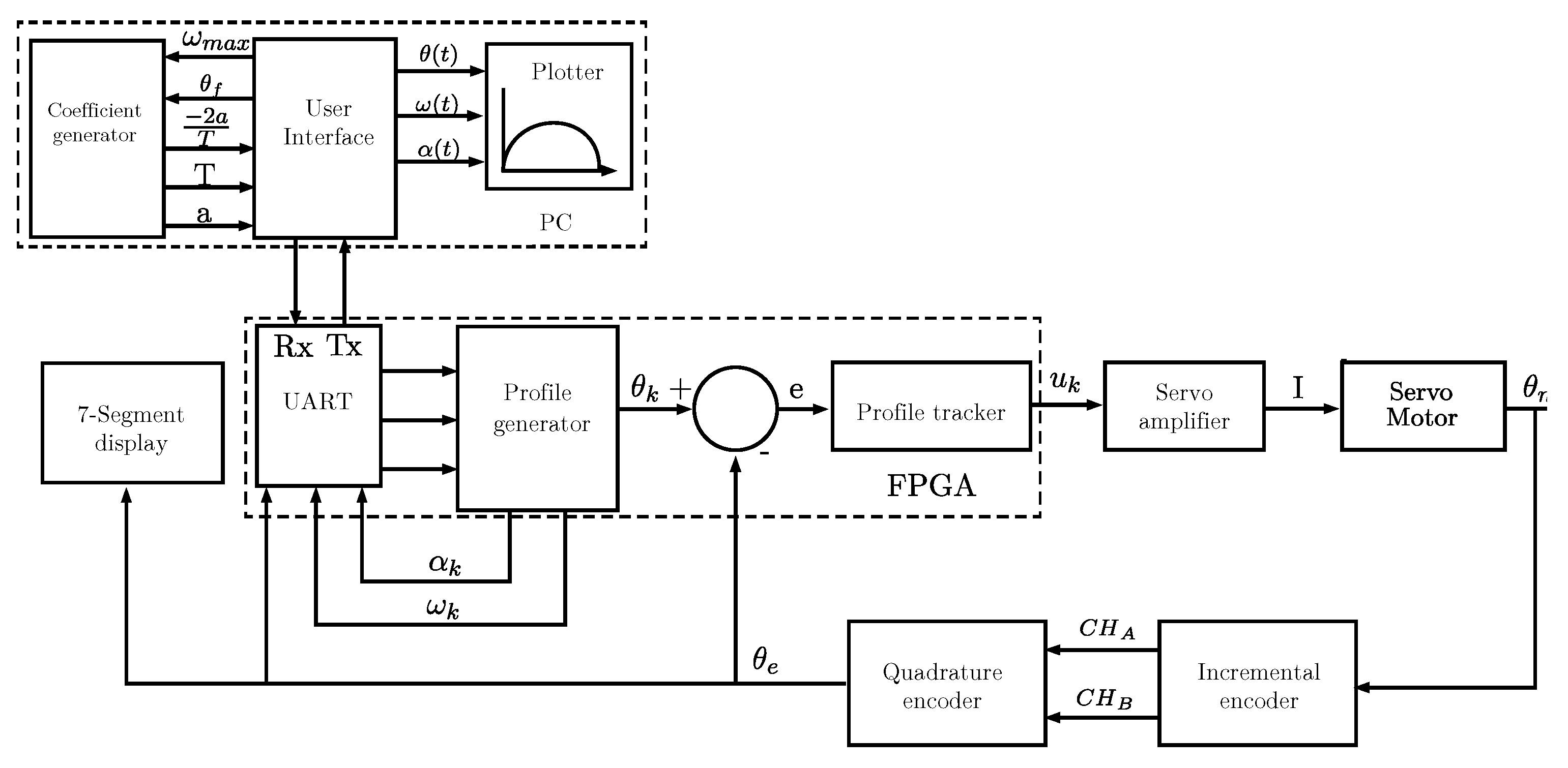Figure 3 and Figure 4 show the system proposed and the general hardware architecture for this work, respectively. The Artix-7 FPGA family is used, which optimized for low power applications requiring serial transceivers and high DSP and logic throughput. Provides the lowest total bill of materials cost for high-throughput, cost-sensitive applications. Also, this FPGA family offers high-end performance at the lowest cost and achievable power. The main characteristics of the device used are presented in

Table 5. Main characteristics of the FPGA used.

Product Family: Artix-7
Project Part: XC7A35TCGP236-1
Logic Cells	Configurable Logic Blocks (CLBs)		DSP48E1 Slices	Block RAM Blocks
	Slices	Max Distributed RAM (KB)		18 KB	36 KB	Max (KB)
33,280	5200	400	90	100	50	1800
CMTs	PCIe	GTPs	XADC Blocks	Total I/O Banks	Max User I/O	Clock Frequency
5	1	4	1	5	250	100 MHz
Power characteristics
Current consumption			Voltage consumption		Power consumption
135 mA			5 V		0.675 W

. The selection of the sampling period was made after carrying out some experiments with higher values. It was also decided to establish a sampling period of 1 ms to simplify the calculations in the internal blocks since it avoids the use of extra blocks (multiplication blocks) when working with the value of 1. Furthermore, in previous investigations the use of this value has been formally justified [37,38].

Block programming is done using VHDL. The blocks are implemented in a flexible and modular way to enable easy customization. It was decided to take advantage of this language advantage due to its magnitude. In this way, if any correction is necessary for any of the blocks, it is not necessary to modify the entire system.

The control flow begins with the user interface, where the type of profile, the maximum velocity and the desired position are selected. Then, the coefficient generator sends the values to the FPGA through a UART transmission-reception module. The profile generator calculates for each instant of time a portion of the final position according to the selected profile. The difference between the profile generator position and the current motor position is sent to the profile tracker; this block induces a current in the motor. The direction of the current is determined by a bit in the received frame and it depends on the sign of the error. The current motor position is measured with the motor encoder and processed with a quadrature module described in the FPGA. The result is used in three ways in the system: as feedback to the profile tracker, as a decimal value displayed on a seven-segment display and as a vector of data transmitted to the interface to graph the motor path.

A Finite State Machine allows control of the two signals given by the encoder. The main clock of the system feeds this component in order to generate a count that could be decremental or incremental, depending on the direction of the shaft of the motor. The two signals from the encoder could reach some MHz, in this sense, when a multi-axe system is requires, the FPGA is a good choice.

The implementation of the profile tracker is done after obtaining a discrete model to add it to the design in the FPGA. As in the velocity profiles, the sampling time $T_s$ is 1 ms. The difference $({\theta }_d-\theta )$ can be expressed as the error $e\left(t\right)$ and rewrite the equation as: $u\left(t\right)=e\left(t\right)$. The block input is the difference between the encoder reading and the desired position. With this circuit, the necessary operations are performed, thus tracing the position requested by the velocity profile generator. The output of the circuit is saturated to couple the result to a 4-bit control action for the motor driver.

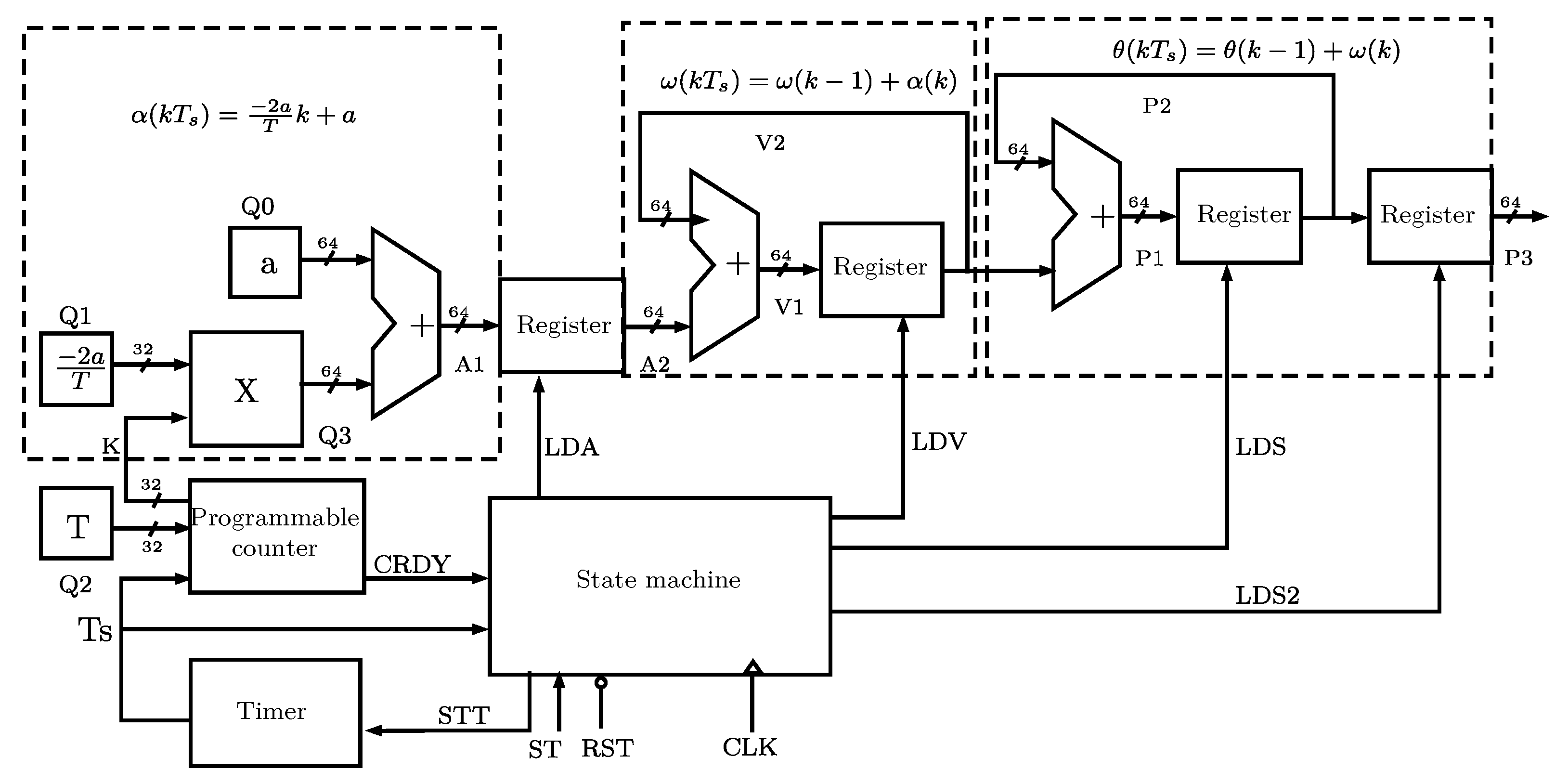
3.1. Implementation of the Parabolic Profile

The calculation of the velocity profiles develops by integrating the acceleration curve once to obtain the velocity and twice to obtain the position. The implementation in the digital system occurs under the same logic, but instead of solving through an analytical integration, numerical integration is used to approximate the desired value at each instant of time. The discrete acceleration equation is obtained by substituting in Equation (1) the value of t for $k{T}_s$, where k is an integer value that increases by 1 for each instant of time and $T_s$ is the sampling period. To simplify operations, it is convenient to select a unit sampling period, in this case 1 ms. The discrete equations are expressed as:

$$\alpha \left(k{T}_s\right)=\frac{-2a}{T}k+a$$

(17)

$$\omega \left(k{T}_s\right)=\omega (k-1)+\alpha \left(k\right)$$

(18)

$$\theta \left(k{T}_s\right)=\theta (k-1)+\omega \left(k\right)$$

(19)

The circuit implemented in the FPGA is described in Figure 5. The inputs for this component are the acceleration curve coefficients (Q0, Q1, Q2), a master clock (CLK), a start signal (ST) and a master reset (RST). The circuit performs the operations established by the numerical integration and gives the output an angular position for each instant of time. The components of the circuit are:

• Time Base: Set the frequency of operations to 1 ms.
• One Programmable counter: Increases its value every millisecond to establish the instant of time the circuit.
• One-State machine: Controls the sequential flow of operations.
• One Multiplier: In conjunction with an adder, it calculates the acceleration.
• Three Adders: Perform the iterative operations for acceleration, velocity and position.
• Four Registers: According to the state machine

3.2. Implementation of the Trapezoidal Profile

The implementation of the trapezoidal profile is carried out in a similar way to Section 3.1 and is shown in Figure 6. The component inputs are acceleration and time period coefficients, a CLK, a ST and an RST. With this circuit it is possible to carry out the rectangular integration that allows us to obtain the angular position of the profile starting from its acceleration. The circuit components are:

• Two-Multiplexers (MUX): The first select the constant value of the acceleration and the second one the constant of time.
• Time Base: Set the sampling period to 1 ms.
• Two-Programmable Counters: The first increase its value every millisecond to establish the instant of time the circuit and the second counter indicates the position in the third part of the trapezoid and serves as a selector for the acceleration and time constants.
• One-State Machine: Controls the sequential flow of operations.
• Two Adders: Perform the iterative operations for velocity and position.
• Three-Registers: According to the state machine they store the data for each instant of time.

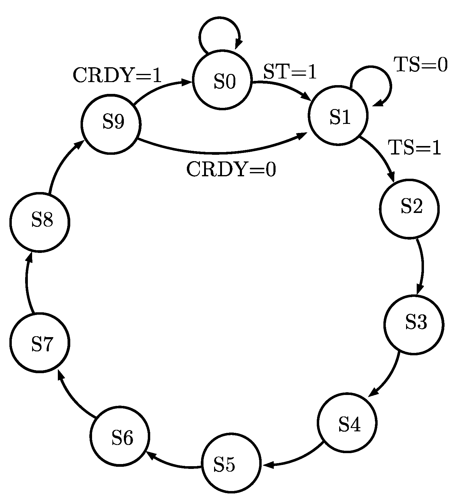
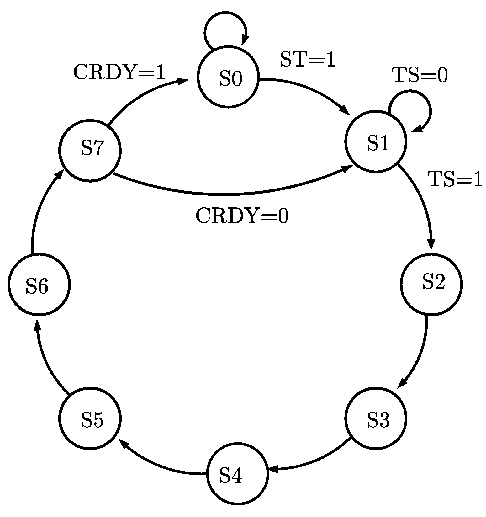
The behavior of the state machine of the trapezoidal and parabolic profiles is described in Figure A1 and Figure A2. The flow of states determines the activation and deactivation of the registers that store the velocity and position values. The only difference between both machines is that for the trapezoidal profile, there is no acceleration register that must be activated and consequently, it consists of only seven states.

3.3. Implementation of the Servo Amplifier

The coupling of the DC motor with the digital controller is achieved through the LMD18245 driver. According to the reference datasheet of the manufacturer, a four-bit digital-to-analog converter (DAC) provides a digital path for controlling the motor current, and, by extension, simplifies implementation of full, half and microstep stepper motor drives. For higher resolution applications, an external DAC can be used. However, the accuracy that is achieved with 4 bits is sufficient for the application developed. The main function of the driver is to control the current supply that the DC motor receives at each instant of time, which modifies its velocity. The main characteristics of the DC motor and driver used for the experiments in this work are mentioned in

Table 6. Experimental Motor.

Motor Characteristics
Model Motor	Pololu 37D Metal Gearmotor
Operation voltage	12 V
Reduction	131:1
Maximum velocity	80 rpm
Encoder counts (Motor shaft)	64 per revolution
Encoder counts (Output gearbox shaft)	8400 per revolution
Maximum current consumed	5 A
Driver Characteristics (LMD18245)
Temperature	$-40$${}^{°}$C a +125 ${}^{°}$C
Voltage supply	+12 V a +55 V
Voltage of DAC	0 V a +5 V
Maximum continuous current	3 A
Maximum current peak	6 A

.

The current that the driver supplies to the servo motor varies in correspondence to the reference voltage VREF. This voltage is proportionally limited by the decimal value of the 4-bit word formed by pins M4 to M1, where M4 is the most significant bit. This reference is sensed and amplified by the CS OUT pin in combination with the Rs resistor.

The current required to overcome the motor resistance and cause movement is 75 mA. When it reaches the nominal velocity (without load), 150 mA is consumed, and the reference voltage may be less than 5 V. The voltage is adjusted to 1.8 V to take full advantage of the 4-bit resolution that the DAC provides for more precise velocity changes. In the event that a load is added to the motor or replaced by a motor that requires more current, it is only necessary to readjust the reference voltage to increase the range of current supplied.

4. Experimental Results

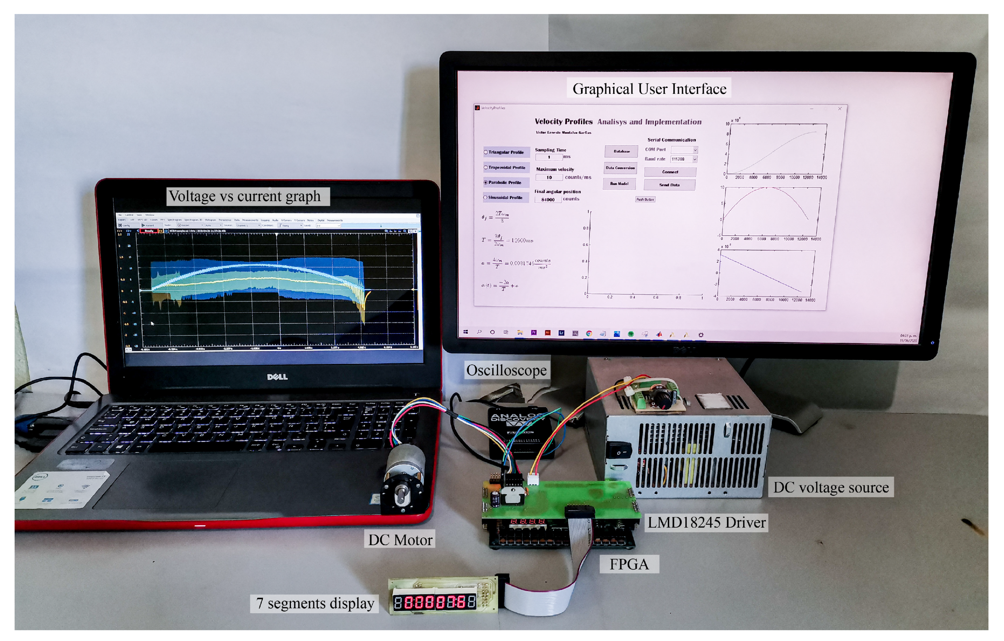
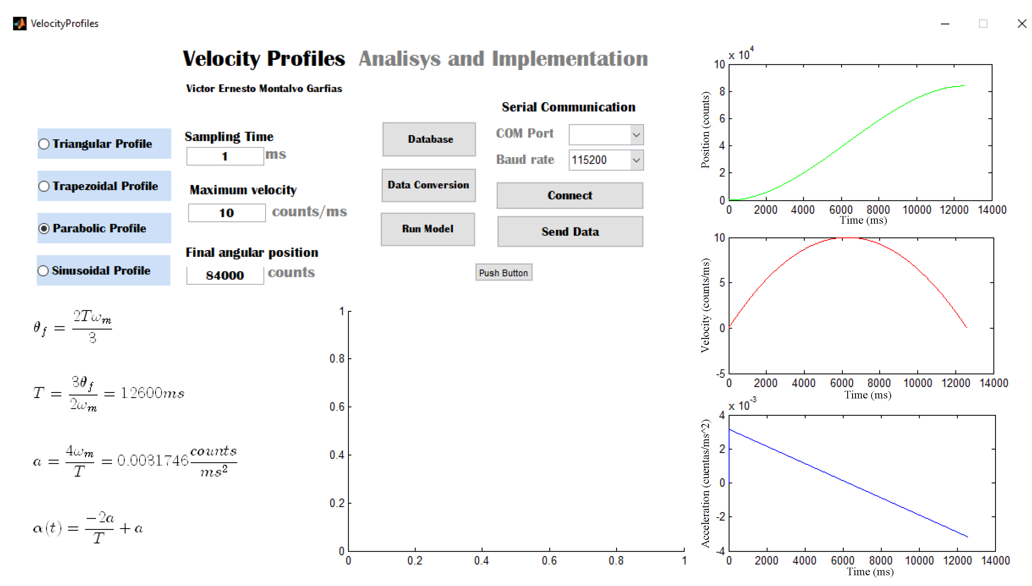
The FPGA assembled on the built PCB is illustrated in Figure 7. Some surface mount components were used to compact the component distribution and increase its wear resistance. The control system interface presented in Figure A5 allow the user to simulate 4 different velocity profiles where they can modify: the maximum motor velocity (given by its specifications), the final angular position and the sampling time. The GUI has been introduced as follows. The GUI helps to the user to set values of the system such as PID gains. Moreover, it permits plotting in real time or offline of the power consumption, and the behavior of the position, among other graphs. It is used the transmitter and receiver virtual serial port from the PC and connected to the FPGA by using three wires.

The precision of a numerical method depends on the iterations that are carried out, the experiment is performed with 15 turns of the parabolic profile and compared with the position obtained through Equation (5). The rectangular numerical method is the one used for the iterations. Before analyzing the results achieved through hardware, studying the error that exists when calculating the angular position with a numerical method is convenient. The results are shown in Figure 8, where the analytical and numerical method is compared with different sampling times by simulation. It is important to note that even with a sampling period 10 times slower than the one used at work (1 ms), the average error remains less than 1%. In a range of 100 ms up to 1 s, the error becomes more significant. The processing velocity in this system is of utmost importance to achieve the results closest to the desired values.

Each test shown in Figure 9 delivers a vector of monitored angular positions in a millisecond. Therefore, it is necessary to adjust the velocity of the RS232 protocol to the maximum supported by the MATLAB IDE: 115200 bps. The interface is not able to graph the received data in real time due to the high-reception velocity. It is important to note that the expected times to reach each angular position are the same for both profiles.

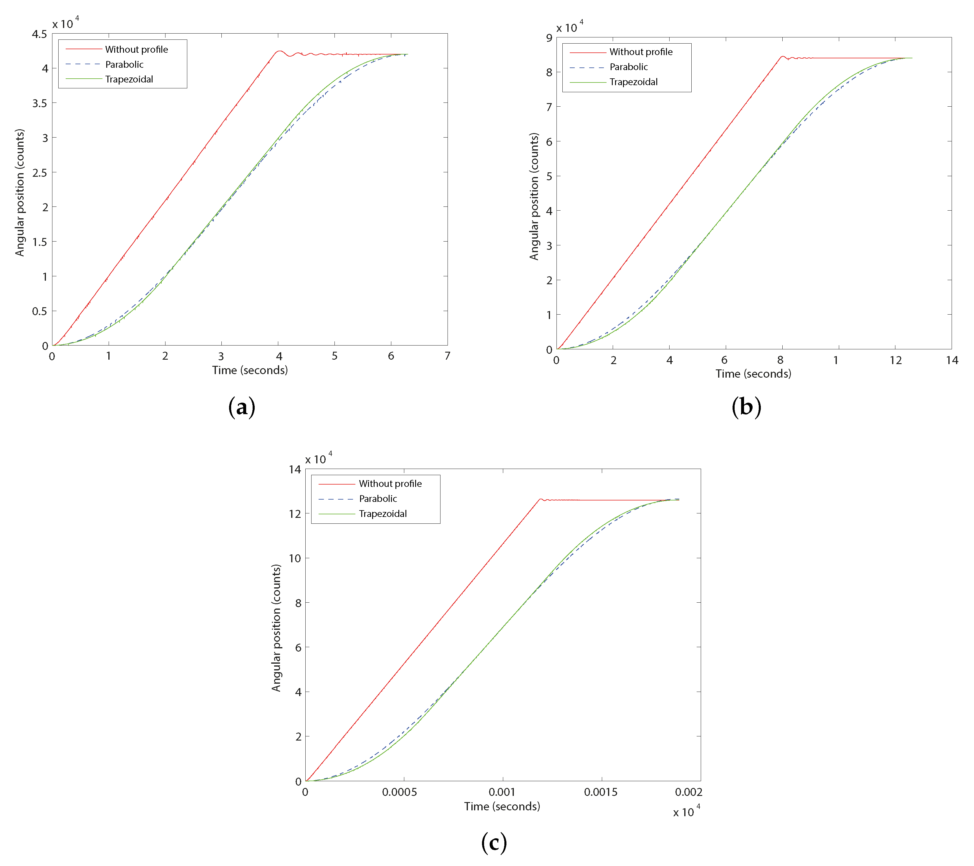
Within the tests carried out on the system, the profile tracker is monitored when velocity profiles are used at its input and when the user directly assigns the position. Maximum engine velocity is a factor that path planning takes into account when calculating the position vector. For this experiment, the velocity is set to 10 per ms, equivalent to 71.4286 rpm, in order not to push the motor operation to the limit. The path followed by the profile tracker without the profile will use the 80 rpm of the engine. The experiments performed are presented in Figure 10.

The results obtained show that the implemented control reaches the established setpoint. Comparisons between the parabolic profile, the trapezoidal profile and a non-profile response are also presented. It can be seen that the parabolic profile reaches the desired position through a smoother curve in an average time of 5 s. It is important to mention that with the implemented control, it is not necessary to use an additional control loop to decrease the steady-state error. The error under standard system operation is less than 1%.

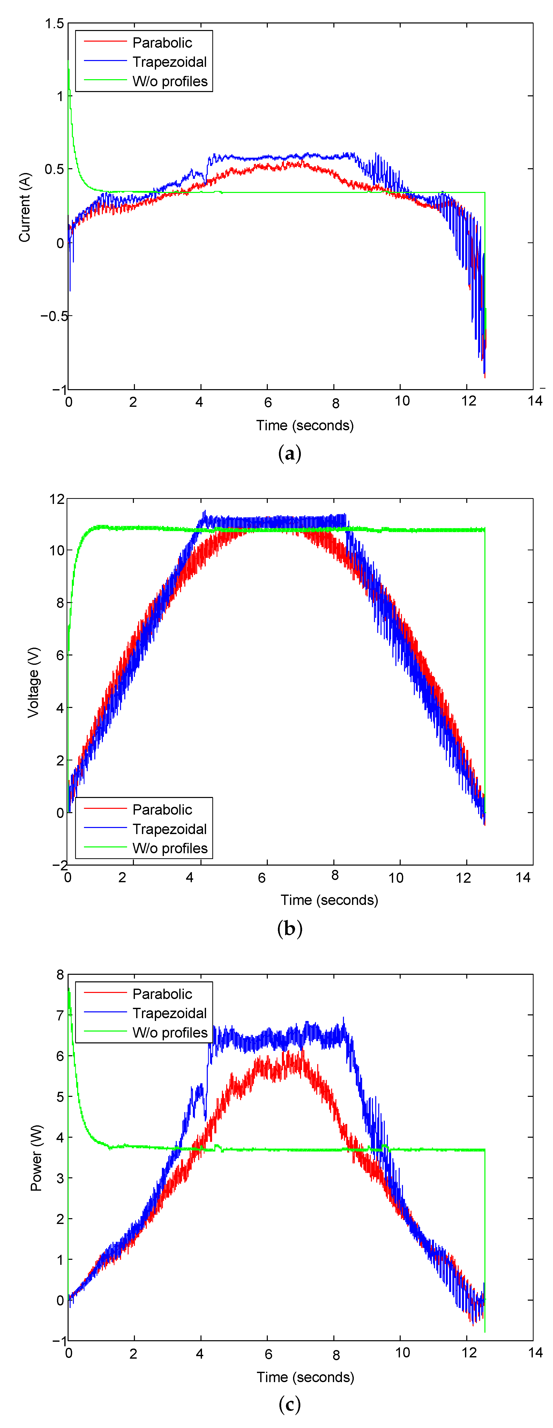
Figure 11 show the current measurement made with the Analog Discovery oscilloscope and MAX471 sensor to measure the power consumption of 10 turns. It should be noted that the function described by the voltages of both experiments is very similar to the velocity curve of each profile.

Table 7. Comparison of the average consumption in both profiles for 10 laps.

Variable	Parabolic Profile	Trapezoidal Profile	No Velocity Profile
Current	0.32 A	0.39 A	0.35 A
Voltage	7.45 V	7.47 V	10.67 V
Power	2.38 W	2.91 W	3.76 W
Energy	29.98 J	36.6 J	47.48 J

presents a comparison of the values of current, voltage and average power for both profiles. Finally, the percentage of use of FPGA resources is shown in Figure 8. It is observed that the consumption of FPGA resources is not excessive, even if improvements are required, they can be carried out without exceeding half the available resources.

The results in the table above show a saving in power consumption of 0.85 W between the trapezoidal profile and the system without a profile. Similarly, 1.38 W is saved using the parabolic profile compared to the system without a profile. For its part, the parabolic profile represents an energy saving of 0.53 W compared to the use of the trapezoidal profile.

Consumption in the FPGA can be reduced by applying different techniques. From a programming standpoint, techniques such as one-hot encoding for state machines and protected evaluation can be implemented while ensuring that logical loops that oscillate are not created. In addition, I/O standards must be chosen appropriately to avoid excessive use of static energy. Finally, an important technique to prevent excessive power usage in the FPGA is to suspend the part of the FPGA that is not in use.

It is important to note that the system responds satisfactorily to tracking the trajectory proposed by both profiles. The average error of the experiments ranges from 2.24% to 4.9%. Although the average error might seem considerable, it is interesting to note that the average error is very high at motor start because the theoretical value vector starts with very small decimal values less than 1 and the encoder gives counts per unit, not per fraction. Therefore, the errors at the beginning of the trajectory are up to almost 100%. However, after approximately the first sixth of the journey, the error is below 1%. The experiment was carried out for three different distances (5, 10 and 15 turns) to verify that the system remains stable at small or long distances and does not increase the value of the error. Regarding energy consumption, it can be seen that as shown in theory, it was significantly lower in the parabolic profile case than the trapezoidal one.

It can be seen that the voltage in both cases (parabolic and trapezoidal profile) was practically the same. However, the significant difference came from the current consumption, being considerably less in the parabolic profile. It can be concluded that the energy consumption in the parabolic profile was 17.3% less than the trapezoidal one. On the other hand, the behavior of energy consumption without a speed profile is considerably higher.

Table 8. Absolute use of FPGA resources.

Absolute Resources Use
Site Type	Used	Fixed	Available	Util %
Slice LUTs	1025	0	20,800	4.93
LUT as Logic	1025	0	20,800	4.93
LUT as Memory	0	0	9600	0.00
Slice Registers	1107	0	41,600	2.66
Register as Flip Flop	1107	0	41,600	2.66
Register as Latch	0	0	41,600	0.00
F7 Muxes	3	0	16,300	0.02
F8 Muxes	0	0	8150	0.00
DSPs	5	0	90	5.56
DSP48E1	5	0	90	5.56
Latency in clock cycles of the implementation
11

shows the consumption of FPGA resources. Furthermore,

Table 9. Comparison of resources consumed in similar works.

Ref.	Flip Flops	Memory	LUTs	Slices	Controller
[39]	3322	-	-	-	Backstepping Sliding-Mode Controller
[40]	-	-	-	1817	PID
[41]	-	232192	20428	-	Adaptative Fuzzy Controller
[37]	2998	-	3792	3048	PID
[42]	-	16384	-	2255	PID

shows a comparison of resources used by the FPGA for similar work. It can be seen that the developed design notably reduces the use of FPGA resources by using multipliers. This aspect enables the implementation of the proposed project in a wide range of similar devices and does not limit its use to devices with high performance.

5. Conclusions

In the paper, a motion control system based on the parabolic velocity profile is developed and implemented and a comparative analysis with the trapezoidal profile is performed. In the selection of the parabolic profile, the behavior of a planned trajectory is observed. The theoretical estimates that address the characteristics of each profile, such as the velocity of response and energy consumption, were verified through experimentation. The difference between the forecast of the mathematical model and the practical example was very low. Among the advantages of the work presented, its modularity stands out. This prototype can be replicated for motors with a consumption of up to 3 A and only requires minor modifications in case of using motors with higher consumption.

Due to the versatility offered by the implementations in digital logic, it was possible to reconfigure the system to observe the behavior with and without the assistance of velocity profiles. The previous approach is verified when the theoretical curve of the profile is very similar to that of the experiment for different angular positions. The main reason for this behavior was the sampling time at 1 ms, which allowed the profiles to show changes of position so small that they did not represent a complication for the profile tracker.

A comparison of the characteristics between the parabolic and trapezoidal profile with a special focus on response time and energy consumption was carried out. Finally, one of the greatest advantages of the parabolic profile compared to the trapezoidal one was demonstrated: a lower energy consumption necessary to complete the desired path. It is important to note that the response time for both profiles was the same and consequently, saving energy did not represent a loss in velocity. With this conclusion, the importance of planning trajectories based on mathematical models that contemplate the focus on variables that significantly impact different mobility applications can be highlighted, in this case: the reduction of costs due to energy savings.

References

1. Payza, O.; Demir, Y.; Aydin, M. Investigation of losses for a Concentrated Winding High-Speed Permanent Magnet-Assisted Synchronous Reluctance Motor for Washing Machine Application. IEEE Trans. Magn. 2018, 54, 1–5. [Google Scholar] [CrossRef]
2. Diao, L.; Tang, J.; Loh, P.C.; Yin, S.; Wang, L.; Liu, Z. An efficient DSP–FPGA-based implementation of hybrid PWM for electric rail traction induction motor control. IEEE Trans. Power Electron. 2018, 33, 3276–3288. [Google Scholar] [CrossRef]
3. Shao, X.; Sun, D. Development of a new robot controller architecture with FPGA-based IC design for improved high-speed performance. IEEE Trans. Ind. Inf. 2007, 3, 312–321. [Google Scholar] [CrossRef]
4. Bellemou, A.M.; García, A.; Castillo, E.; Benblidia, N.; Anane, M.; Álvarez-Bermejo, J.A.; Parrilla, L. Efficient implementation on low-cost SoC-FPGAs of TLSv1.2 protocol with ECC_AES support for secure IoT coordinators. Electronics 2019, 8, 1238. [Google Scholar] [CrossRef] [Green Version]
5. Cerezo, J.; Morales, E.; Plaza, J. Control system in open-source FPGA for a self-balancing robot. Electronics 2019, 8, 198. [Google Scholar] [CrossRef] [Green Version]
6. Ala, G.; Caruso, M.; Miceli, R.; Pellitteri, F.; Schettino, G.; Trapanese, M.; Viola, F. Experimental investigation on the performances of a multilevel inverter using a field programmable gate array-based control system. Energies 2019, 12, 1016. [Google Scholar] [CrossRef] [Green Version]
7. Krim, S.; Gdaim, S.; Mtibaa, A.; Mimouni, M.F. FPGA-based real-time implementation of a direct torque control with second-order sliding mode control and input–output feedback linearisation for an induction motor drive. IET Electr. Power Appl. 2020, 14, 480–491. [Google Scholar] [CrossRef]
8. Bai, H.; Liu, C.; Ma, R.; Paire, D.; Gao, F. Device-level modelling and FPGA-based real-time simulation of the power electronic system in fuel cell electric vehicle. IET Power Electron. 2019, 12, 3479–3487. [Google Scholar] [CrossRef]
9. Wirtz, S.; Cunha, A.; Labusch, M.; Marzun, G.; Barcikowski, S.; Söffker, D. Development of a low-cost FPGA-based measurement system for real-time processing of acoustic emission data: Proof of concept using control of pulsed laser ablation in liquids. Sensors 2018, 18, 1775. [Google Scholar] [CrossRef] [Green Version]
10. Nicolas-Apruzzese, J.; Lupon, E.; Busquets-Monge, S.; Conesa, A.; Bordonau, J.; García-Rojas, G. FPGA-based controller for a permanent-magnet synchronous motor drive based on a four-level active-clamped DC-AC converter. Energies 2018, 11, 2639. [Google Scholar] [CrossRef] [Green Version]
11. Ricco, M.; Mathe, L.; Monmasson, E.; Teodorescu, R. FPGA-based implementation of MMC control based on sorting networks. Energies 2018, 11, 2394. [Google Scholar] [CrossRef] [Green Version]
12. Parrilla, L.; Castillo, E.; Morales, D.; García, A. Hardware activation by means of PUFs and elliptic curve cryptography in field-programmable devices. Electronics 2016, 5, 5. [Google Scholar] [CrossRef] [Green Version]
13. Jeppesen, B.P.; Rajamani, M.; Smith, K.M. Enhancing functional safety in FPGA-based motor drives. J. Eng. 2019, 2019, 4580–4584. [Google Scholar] [CrossRef]
14. Idkhajine, L.; Monmasson, E.; Naouar, M.W.; Prata, A.; Bouallaga, K. Fully integrated FPGA-based controller for synchronous motor drive. IEEE Trans. Ind. Electron. 2009, 56, 4006–4017. [Google Scholar] [CrossRef]
15. Martinez-Prado, M.; Franco-Gasca, A.; Herrera-Ruiz, G.; Soto-Dorantes, O. Multi-axis motion controller for robotic applications implemented on an FPGA. Int. J. Adv. Manuf. Technol. 2012, 67, 2367–2376. [Google Scholar] [CrossRef]
16. García Martínez, J.R.; Rodríguez Reséndiz, J.; Martínez Prado, M.A.; Cruz Miguel, E.E. Assessment of jerk performance s-curve and trapezoidal velocity profiles. In Proceedings of the 2017 XIII International Engineering Congress (CONIIN), Santiago de Queretaro, Mexico, 15–17 May 2017; pp. 1–7. [Google Scholar] [CrossRef]
17. Rew, K.; Kim, K. A closed-form solution to asymmetric motion profile allowing acceleration manipulation. IEEE Trans. Ind. Electron. 2010, 57, 2499–2506. [Google Scholar] [CrossRef]
18. Yoon, H.J.; Chung, S.Y.; Kang, H.S.; Hwang, M.J. Trapezoidal motion profile to suppress residual vibration of flexible object moved by robot. Electronics 2019, 8, 30. [Google Scholar] [CrossRef] [Green Version]
19. Bangji, W.; Qingxiang, L.; Lei, Z.; Yanrong, Z.; Xiangqiang, L.; Jianqiong, Z. Velocity profile algorithm realization on FPGA for stepper motor controller. In Proceedings of the 2011 IEEE 2nd International Conference on Artificial Intelligence, Management Science and Electronic Commerce (AIMSEC), Dengleng, China, 8–10 August 2011. [Google Scholar] [CrossRef]
20. Gedik, A.; Bilgin, E.; Lav, A.H.; Artan, R. An investigation into the effect of parabolic speed hump profiles on ride comfort and driving safety under variable vehicle speeds: A campus experience. Sustain. Cities Soc. 2019, 45, 413–421. [Google Scholar] [CrossRef]
21. Grassmann, R.M.; Burgner-Kahrs, J. Quaternion-based smooth trajectory generator for via poses in SE (3) considering kinematic limits in cartesian space. IEEE Robot. Autom. Lett. 2019, 4, 4192–4199. [Google Scholar] [CrossRef]
22. Piazzi, A.; Visioli, A. Global minimum-jerk trajectory planning of robot manipulators. IEEE Trans. Ind. Electron. 2000, 47, 140–149. [Google Scholar] [CrossRef] [Green Version]
23. Biagiotti, L.; Melchiorri, C. Trajectory Planning for Automatic Machines and Robots; Springer Science & Business Media: Berlin/Heidelberg, Germany, 2008. [Google Scholar]
24. Osornio-Rios, R.A.; de Jesús Romero-Troncoso, R.; Herrera-Ruiz, G.; Castañeda-Miranda, R. FPGA implementation of higher degree polynomial acceleration profiles for peak jerk reduction in servomotors. Robot. Comput.-Integr. Manuf. 2009, 25, 379–392. [Google Scholar] [CrossRef]
25. Heo, H.J.; Son, Y.; Kim, J.M. A trapezoidal velocity profile generator for position control using a feedback strategy. Energies 2019, 12, 1222. [Google Scholar] [CrossRef] [Green Version]
26. García-Martínez, J.R.; Rodríguez-Reséndiz, J.; Cruz-Miguel, E.E. A new seven-segment profile algorithm for an open source architecture in a hybrid electronic platform. Electronics 2019, 8, 652. [Google Scholar] [CrossRef] [Green Version]
27. Bai, Y.; Chen, X.; Sun, H.; Yang, Z. Time-optimal freeform S-curve profile under positioning error and robustness constraints. IEEE/ASME Trans. Mechatron. 2018, 23, 1993–2003. [Google Scholar] [CrossRef]
28. de Almeida, A.T.; Fong, J.; Falkner, H.; Bertoldi, P. Policy options to promote energy efficient electric motors and drives in the EU. Renew. Sustain. Energy Rev. 2017, 74, 1275–1286. [Google Scholar] [CrossRef]
29. Ma, Z.; Asmussen, A.; Jørgensen, B. Industrial consumers’ smart grid adoption: Influential factors and participation phases. Energies 2018, 11, 182. [Google Scholar] [CrossRef] [Green Version]
30. Samad, T.; Kiliccote, S. Smart grid technologies and applications for the industrial sector. Comput. Chem. Eng. 2012, 47, 76–84. [Google Scholar] [CrossRef]
31. Ha, C.; Lee, D. Analysis of embedded prefilters in motion profiles. IEEE Trans. Ind. Electron. 2018, 65, 1481–1489. [Google Scholar] [CrossRef]
32. Nguyen, K.D.; Ng, T.C.; Chen, I.M. On algorithms for planning s-curve motion profiles. Int. J. Adv. Robot. Syst. 2008, 5, 11. [Google Scholar] [CrossRef]
33. Shin, S.C.; Choi, C.H.; Youm, J.H.; Lee, T.K.; Won, C.Y. Position control of PMSM using jerk-limited trajectory for torque ripple reduction in robot applications. In Proceedings of the IECON 2012—38th Annual Conference on IEEE Industrial Electronics Society, Montreal, QC, Canada, 25–28 October 2012. [Google Scholar] [CrossRef]
34. Ha, C.W.; Rew, K.H.; Kim, K.S. Robust zero placement for motion control of lightly damped systems. IEEE Trans. Ind. Electron. 2013, 60, 3857–3864. [Google Scholar] [CrossRef]
35. Nguyen, K.D.; Chen, I.M.; Ng, T.C. Planning algorithms for s-curve trajectories. In Proceedings of the 2007 IEEE/ASME international conference on advanced intelligent mechatronics, Zurich, Switzerland, 4–7 September 2007. [Google Scholar] [CrossRef]
36. Karnavas, Y.L.; Topalidis, A.S.; Drakaki, M. Development and implementation of a low cost μC- based brushless DC motor sensorless controller: A practical analysis of hardware and software aspects. Electronics 2019, 8, 1456. [Google Scholar] [CrossRef] [Green Version]
37. Martinez-Prado, M.A.; Rodriguez-Resendiz, J.; Gomez-Loenzo, R.A.; Herrera-Ruiz, G.; Franco-Gasca, L.A. An FPGA-based open architecture industrial robot controller. IEEE Access 2018, 6, 13407–13417. [Google Scholar] [CrossRef]
38. Martínez-Prado, M.A.; Rodríguez-Reséndiz, J.; Gómez-Loenzo, R.A.; Camarillo-Gómez, K.A.; Herrera-Ruiz, G. Short informative title: Towards a new tendency in embedded systems in mechatronics for the engineering curricula. Comput. Appl. Eng. Educ. 2019, 27, 603–614. [Google Scholar] [CrossRef] [Green Version]
39. Lin, F.J.; Chang, C.K.; Huang, P.K. FPGA-based adaptive backstepping sliding-mode control for linear induction motor drive. IEEE Trans. Power Electron. 2007, 22, 1222–1231. [Google Scholar] [CrossRef]
40. Shao, X.; Sun, D. An FPGA based motion control IC and its application to robotic manipulators. In Proceedings of the 2006 9th International Conference on Control, Automation, Robotics and Vision, Singapore, 5–8 December 2006. [Google Scholar] [CrossRef]
41. Kung, Y.S.; Li, S.W. FPGA-realization of a motion control IC for X-Y table with adaptive fuzzy control. In Proceedings of the 2010 11th IEEE International Workshop on Advanced Motion Control (AMC), Nagaoka, Japan, 21–24 March 2010. [Google Scholar] [CrossRef]
42. Dong, J.; Wang, T.; Li, B.; Liu, Z.; Yu, Z. An FPGA-based low-cost VLIW floating-point processor for CNC applications. Microprocess. Microsyst. 2017, 50, 14–25. [Google Scholar] [CrossRef]
Figure 1. Curves obtained for the parabolic profile: (a) Acceleration, (b) Velocity, (c) Position.
Electronics 09 01301 g001
Figure 2. Curves obtained for the trapezoidal profile: (a) Acceleration, (b) Velocity, (c) Position.
Electronics 09 01301 g002
Figure 3. General block diagram of the implemented system.
Electronics 09 01301 g003
Figure 4. Block diagram of the implemented control loop.
Electronics 09 01301 g004
Figure 5. Block diagram of the discrete parabolic profile.
Electronics 09 01301 g005
Figure 6. Block diagram of the discrete trapezoidal profile.
Electronics 09 01301 g006
Figure 7. Low-cost platform for industrial applications based on FPGA.
Electronics 09 01301 g007
Figure 8. Simulation comparison between analytical method and numerical method for 15 turns in parabolic profile.
Electronics 09 01301 g008
Figure 9. Experimental comparison of the position control of both profiles for 15 turns. (a) Parabolic velocity profile. (b) Parabolic error. (c) Trapezoidal velocity profile. (d) Trapezoidal error.
Electronics 09 01301 g009
Figure 10. Experimentally obtained response with and without profiles. (a) 5 turns. (b) 10 turns. (c) 15 turns.
Electronics 09 01301 g010
Figure 11. Comparison of voltage, current and power in both profiles for 10 turns. (a) Current. (b) Voltage. (c) Power.
Electronics 09 01301 g011