Discrete-Time Neural Control of Quantized Nonlinear Systems with Delays: Applied to a Three-Phase Linear Induction Motor

Abstract

This work introduces a neural-feedback control scheme for discrete-time quantized nonlinear systems with time delay. Traditionally, a feedback controller is designed under ideal assumptions that are unrealistic for real-work problems. Among these assumptions, they consider a perfect communication channel for controller inputs and outputs; such a perfect channel does not consider delays, or noise introduced by the sensors and actuators even if such undesired phenomena are well-known sources of bad performance in the systems. Moreover, traditional controllers are also designed based on an ideal plant model without considering uncertainties, disturbances, sensors, actuators, and other unmodeled dynamics, which for real-life applications are effects that are constantly present and should be considered. Furthermore, control system design implemented with digital processors implies sampling and holding processes that can affect the performance; considering and compensating quantization effects of measured signals is a problem that has attracted the attention of control system researchers. In this paper, a neural controller is proposed to overcome the problems mentioned above. This controller is designed based on a neural model using an inverse optimal approach. The neural model is obtained from available measurements of the state variables and system outputs; therefore, uncertainties, disturbances, and unmodeled dynamics can be implicitly considered from the available measurements. This paper shows the performance and effectiveness of the proposed controller presenting real-time results obtained on a linear induction motor prototype. Also, this work includes stability proof for the whole scheme using the Lyapunov approach.

1. Introduction

Traditionally, a control system is designed based on many assumptions, which are rarely satisfied in real-life systems. One of these assumptions is a mathematical model that perfectly represents the behavior of the system. However, most of the used mathematical models do not consider disturbances, uncertainties, parametric variations, unmodeled dynamics, among other issues. Moreover, there is the assumption that the state measurements and calculated control signals are transmitted through ideal communication channels without the noise of sensors, signal delays, and packet losses, which are phenomena that are present in the day to day systems. These factors are sources that need to be compensated adequately by the controller to have proper performance and avoid stability problems.

In control system design, the existence of delays can severely degrade the performance of the controllers, as well as causing a loss in system stability, among other undesirable effects [1,2,3]. Ignoring measurement noise when designing a controller can cause undesired performance or system failure, especially for systems with high sensitivity to uncertainties [4]. Furthermore, control system design implemented with digital processors implies sampling and holding processes; both operations can severely affect the performance of the designed controller [5]. Moreover, the design of controllers that consider and compensate quantization effects of measured signals is a problem that has attracted the attention of control system researchers for many years [6], which is highly relevant due to the importance that the investigation of networked control systems has gained recently [7].

Previous research [8,9] show a successful trajectory tracking based on ideal conditions. Also, the use of intelligent system techniques has allowed the control schemes to be designed in a manner inspired by nature. These complex dynamic systems include robotic navigation, synchronization, complex networks, control of complex processes, smart grids, among others, see [10,11,12,13]. Mainly, neural networks and fuzzy logic systems have made significant progress in designing solutions for complex control systems. In [14], deterministic learning is presented to identify nonlinear dynamic systems based on sampled data sequences with simulation results applied to chaotic systems using radial basis neural networks. In [15], a backstepping controller based on a fuzzy observer for the control of a nonlinear system with strict second-order feedback is presented. In [16], an adaptive neural controller for uncertain nonlinear systems with state and input restrictions is presented, with simulation-level results, for a single-link robot.

Regarding the design of controllers considering quantization, in [17], a feedback control with static quantization is presented for discrete-time systems. In [18], a feedback optimal neural controller is designed for nonlinear systems quantized in discrete time with input constraints. In [19], the case of the stabilization of nonlinear systems based on three-layer neural networks as a universal approximator of dynamic systems is considered. In [20], a quantized adaptive controller for uncertain nonlinear systems in the presence of external disturbances is presented. Another current approach is described in [21], which shows the design of an adaptive fault-tolerant controller with input prescribed performance for trajectory tracking with quantization and unknown control directions. A similar problem is analyzed in [3], where the use of a Takagi–Sugeno fuzzy controller is proposed for systems in the network under actuator saturation, measurement noise, and quantization. In [22], an inverse optimal neural controller is presented for nonlinear discrete systems considering disturbances; in [2], time delays, as well as disturbances, are considered in neural controller design. Nevertheless, it must be noted that none of the above-referenced works include a real-time implementation of a controller, which considers at the same time disturbances, noise, delays, and quantization for a system with an unknown model.

Please note that all the controllers mentioned above only include simulation-level results due to the difficulty of adequately measuring the effects referred above and the complexity of their corresponding stability analysis.

Motivated by these facts, this paper presents the design and implementation of a discrete-time neural controller for quantized nonlinear systems with delays and measurement noise, while presenting disturbances, uncertainties and unmodeled dynamics, also, without the need for prior knowledge of the system model or the need to estimate its bounds, nor nominal models. Accordingly, the main contributions of this paper can be defined as follows: First, it is designed a neural controller for uncertain nonlinear systems under the inverse optimality approach; second, such controller is implemented in real time and third stability proof of the entire system is included using a Lyapunov approach considering: quantization of the state and input signals, unknown state delays, measurement noise, external disturbances, uncertainties, unknown model, among others.

This paper is organized as follows: Section 2 includes some preliminary concepts and problem statement. Section 3 describes the design of the discrete-time neural controller for uncertain nonlinear systems, including the Lyapunov proof. Section 4 presents real-time results, and in Section 5, conclusions about our proposal are presented.

2. Problem Statement

We propose to solve the problem of designing a discrete-time neural controller for quantized uncertain nonlinear systems under the presence of delays, without the need to have prior knowledge of the system model. First, essential definitions are considered below to define a neural model that considers all the dynamics caused by the above-mentioned phenomena. Based on such a model, a controller is designed to achieve trajectory tracking.

2.1. System Definition

Let us consider a discrete-time unknown nonlinear delayed system that can be written in an affine form as follows:

$$\begin{array}{ccc}\hfill x\left(k+1\right)& =& f\left(x\left(k\right)\right)+g\left(x\left(k\right)\right)u\left(k\right),\hfill \\ \hfill y\left(k\right)& =& Cx\left(k\right),\hfill \end{array}$$

(1)

where $x\left(k\right)\in {\Re }^n$ is the state of the system, $u\left(k\right)\in {\Re }^m$ is the control input, and $f\left(x\left(k\right)\right):{\Re }^n\to {\Re }^n$ and $g\left(x\left(k\right)\right):{\Re }^n\to {\Re }^{n\times m}$ are smooth maps. Without loss of generality, system (1) is assumed to have an equilibrium point at $x\left(k\right)=0$.

Then (1) can be rewritten as:

$$\begin{array}{ccc}\hfill x\left(k-l\right)& =& {\left[\begin{array}{ccccc}{x}_1\left(k\right)& \dots & x_i\left(k\right)& \dots & x_n\left(k\right)\end{array}\right]}^{\top },\hfill \\ \hfill d\left(k\right)& =& {\left[\begin{array}{ccccc}{d}_1\left(k\right)& \dots & d_i\left(k\right)& \dots & d_n\left(k\right)\end{array}\right]}^{\top },\hfill \\ \hfill x_i\left(k+1\right)& =& f_i\left(x\left(k\right)\right)+g_i\left(x\left(k\right)\right)u\left(k\right),\hfill \\ \hfill y\left(k\right)& =& Cx\left(k\right).\hfill \end{array}$$

(2)

2.2. Inverse Optimal Control Methodology

The main idea behind inverse optimal control methodology is to design a control law and then the cost functional [23]. For the state feedback control synthesis, it is necessary to fulfill the following Assumption:

Assumption 1.

The full state x (k) of system (1) is available.

If the full state vector is not available for measurement, Assumption 1 may be fulfilled using a state estimator considering the discrete-time separation principle for nonlinear systems.

The trajectory tracking problem can be solved as a regulation problem for an error system that should be regulated to the origin. For such transformation, an auxiliary error system should be defined using error equations and its dynamics, in this case, let us consider the trajectory tracking error as:

$$\psi \left(k\right)=x\left(k\right)-x_d\left(k\right),$$

(3)

with $x_d\left(k\right)$ the desired trajectory for $x\left(k\right)$, it is important to note that the proposed controller only requires the knowledge of $x_d\left(k+1\right)$ and there is no longer a restriction for $x_d$, which is an improvement with respect to other controllers. Let us propose a control Lyapunov function (CLF) as

$$V\left(\psi \left(k\right)\right)=\frac{1}{2}{\psi }^T\left(k\right)\mathcal{P}\psi \left(k\right),\mathcal{P}={\mathcal{P}}^T>0,$$

(4)

to ensure the stability of the trajectory tracking error (3), which will be achieved by defining an appropriate matrix $\mathcal{P}$. Instead of solving the Hamilton-Jacobi-Bellman (HJB) equation, the inverse optimal control synthesis is based on the knowledge of $V\left(\psi \left(k\right)\right)$. The control law $u\left(k\right)$ can be defined as:

$$\begin{array}{ccc}u\left(k\right)\hfill & =& -\frac{1}{2}{\mathcal{R}}^{-1}\left(\psi \left(k\right)\right)g^T\left(\psi \left(k\right)\right)\frac{\partial V\left(\psi \left(k+1\right)\right)}{\partial \psi \left(k+1\right)}\hfill \\ & =& -\frac{1}{2}{\left(\mathcal{R}\left(\psi \left(k\right)\right)+\frac{1}{2}{g}^T\left(\psi \left(k\right)\right)\mathcal{P}g\left(\psi \left(k\right)\right)\right)}^{-1}{g}^T\left(\psi \left(k\right)\right)\mathcal{P}{f}^T\left(\psi \left(k\right)\right),\hfill \end{array}$$

(5)

where $\mathcal{R}\left(\psi \left(k\right)\right)={\mathcal{R}}^T\left(\psi \left(k\right)\right)>0$ is a weighting matrix whose entries can be functions of the system state or can be fixed, i.e., it can be selected as $\mathcal{R}\left(\psi \left(k\right)\right)=\mathcal{R}$. Since $\mathcal{P}$ and $\mathcal{R}\left(\psi \left(k\right)\right)$ are positive definite and symmetric matrices, the existence of the inverse in (5) is ensured [22,23]. Now, the control synthesis goal is to obtain an appropriate matrix $\mathcal{P}$ for (5) such that $\mathcal{P}={\mathcal{P}}^T>0$, and its values are determined heuristically in order to improve trajectory tracking performance; stability analysis guarantees optimality of the inverse optimal controller. The following theorem establishes a sufficient condition for the matrix $\mathcal{P}$ regarding inverse optimal control.

Theorem 1.

([23]). Consider the system (1). If there exists a matrix $\mathcal{P}={\mathcal{P}}^T>0$ such that the following inequality holds:

$$V_f\left(\psi \left(k\right)\right)-\frac{1}{4}{\mathcal{P}}_1^T\left(\psi \left(k\right)\right){\left(\mathcal{R}\left(\psi \left(k\right)\right)+{\mathcal{P}}_2\left(\psi \left(k\right)\right)\right)}^{-1}{\mathcal{P}}_1\left(\psi \left(k\right)\right)\le -{\psi }^T\left(k\right)\mathcal{Q}\psi \left(k\right),$$

where

$$\begin{array}{ccc}\hfill V_f\left(\psi \left(k\right)\right)& =& \frac{1}{2}{f}^T\left(\psi \left(k\right)\right)\mathcal{P}f\left(\psi \left(k\right)\right)-V\left(\psi \left(k\right)\right),\hfill \\ \hfill {\mathcal{P}}_1\left(\psi \left(k\right)\right)& =& g^T\left(\psi \left(k\right)\right)\mathcal{P}f\left(\psi \left(k\right)\right),\hfill \\ \hfill {\mathcal{P}}_2\left(\psi \left(k\right)\right)& =& \frac{1}{2}{g}^T\left(\psi \left(k\right)\right)\mathcal{P}g\left(\psi \left(k\right)\right),\hfill \end{array}$$

(6)

$V\left(\psi \left(k\right)\right)$ as defined in (4) and $\mathcal{Q}={\mathcal{Q}}^T>0$, then, the equilibrium point $\psi \left(k\right)=0$ from the system (1) is globally exponentially stabilized by the control law (5). Moreover, this control law is inverse optimal in the sense that it minimizes the meaningful functional given by

$$J\left(k\right)=\sum _{k=0}^{\infty }\left(l\left(\psi \left(k\right)\right)+u^T\left(k\right)\mathcal{R}\left(\psi \left(k\right)\right)u\left(k\right)\right),$$

(7)

with $l\left(\psi \left(k\right)\right)=-V\left(\psi \left(k+1\right)\right)+V\left(\psi \left(k\right)\right)-u^{*T}\mathcal{R}\left(\psi \left(k\right)\right)u^{*}\left(k\right)$.

Proof. 

For the detailed proof of Theorem 1, we refer the reader to [23].  □

System (1), is described in an affine form, which is not a trivial requirement for general nonlinear systems, mainly for unknown nonlinear systems. Therefore, in this paper, a neural identifier is used to provide an accurate model for the nonlinear system to be controlled. The model should be presented in a block control form [23].

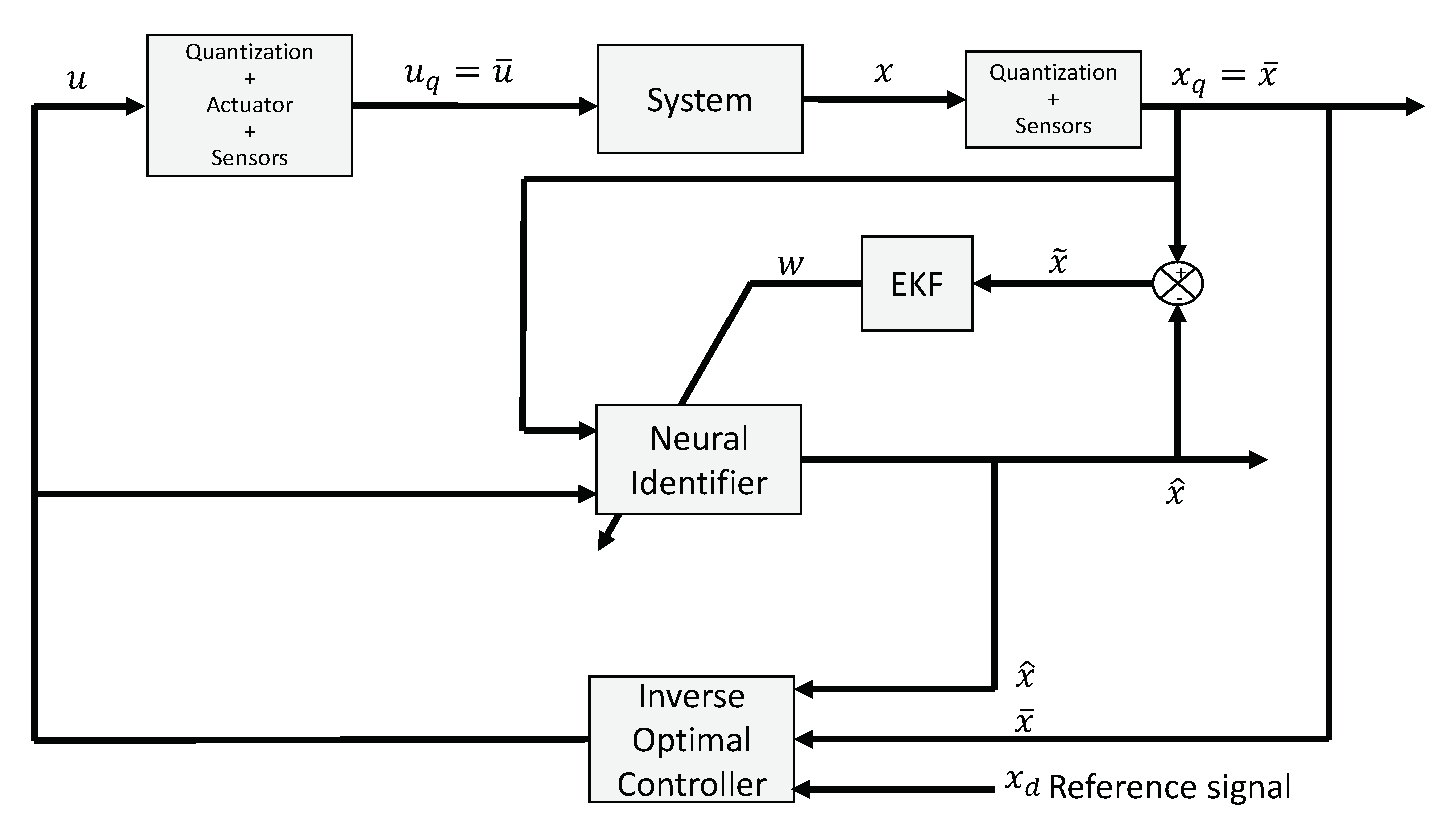
2.3. Quantizers in a Control Loop

Different kinds of quantizers are considered in the literature. These include static, dynamic, uniform, logarithmic, hysteresis, among other kinds of quantizers. However, in practice, uniform quantizers are typically used, mainly due to technological constraints, although other quantizers may be advantageous for analytical purposes [7]. In our work, a dynamic uniform quantizer is considered.

In this paper, the general quantizer is defined as the one described in [17]. Let us assume that $v\in {\Re }^s$ and that there exist numbers $M>0$ and $D>0$ such that the following condition holds:

$$\left|q\right(v)-v|\le D,\mathrm{if}\left|v\right|\le M,$$

(8)

where v is the signal to be quantized, $q\left(v\right)$ is the signal after quantization, M denotes the range of the quantizer, and D stands for the quantization error boundary of the quantizer. In the developed control strategy, we consider the one-parameter family of quantizers that can be defined as:

$$q_{\mu }\left(v\right)=\mu q\left(\frac{v}{\mu }\right),$$

(9)

where $\mu >0$ is the parameter of the quantizer which can be computed independently, therefore $q\left(v\right)$ in (8) can be defined as (9), although, in this paper, it is considered unknown. Let us consider the quantized measured state signal and the quantized control input signal in the following form:

$$x_q\left(k\right)=q_{{\mu }_x}\left(x\left(k\right)\right)={\mu }_{x}q\left(\frac{x\left(k\right)}{{\mu }_x}\right),$$

(10)

$$u_q\left(k\right)=q_{{\mu }_u}\left(u\left(k\right)\right)={\mu }_{u}q\left(\frac{u\left(k\right)}{{\mu }_u}\right),$$

(11)

where $q_{{\mu }_{*}}\left(·\right)$ is a dynamic quantizer defined by (9), which is comprised of a dynamic scaling ${\mu }_{*}$ and by a static quantizer $q\left(·\right)$ defined by (8) with range $M_{*}$ and error $D_{*}$ [18].

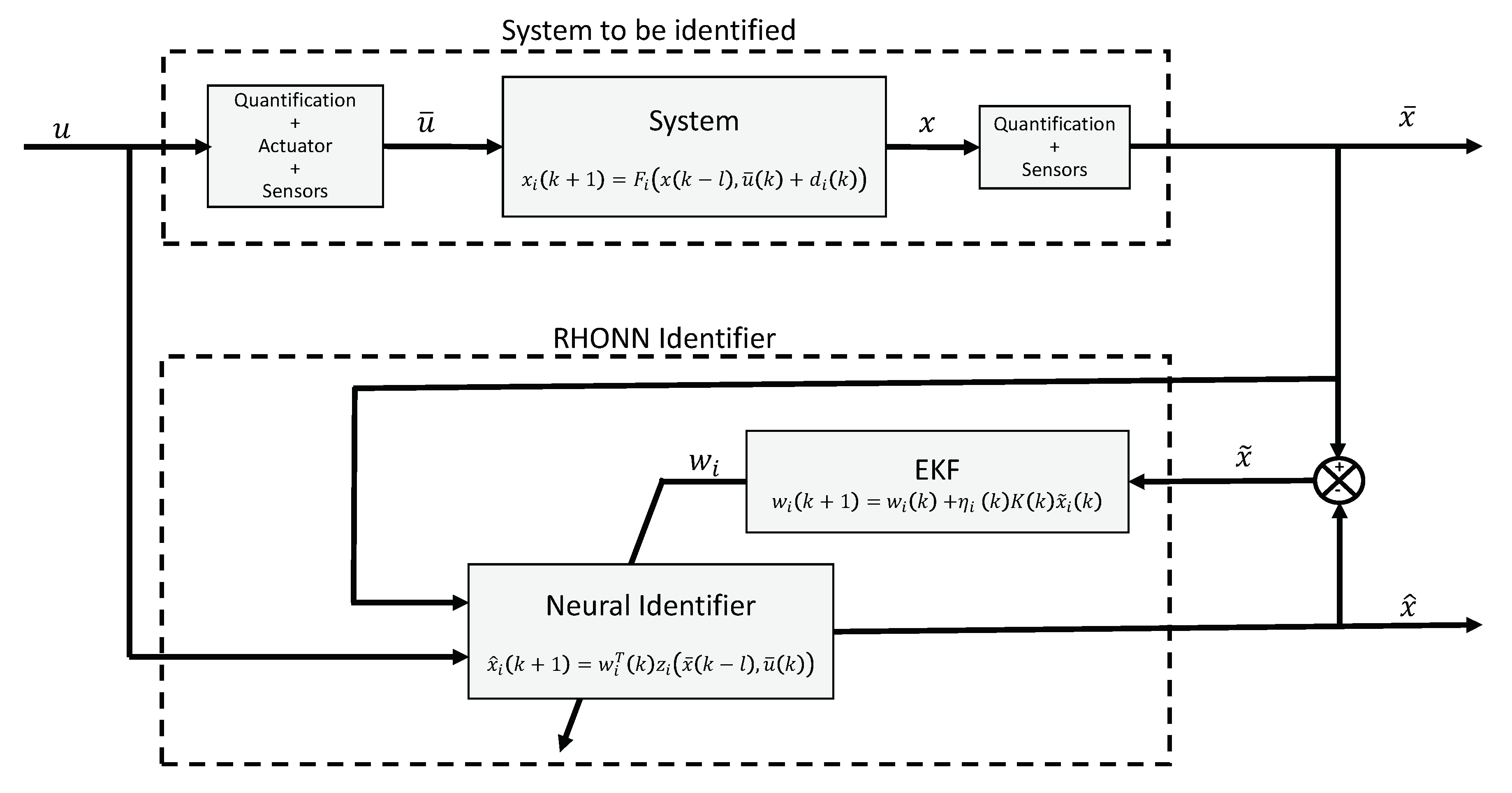
3. Neural Controller Design

The inverse optimal controller defined in the previous section is defined for an ideal system. Such a system is considered ideal since the calculated control law is directly applied to the system without the actuator limitations and input quantization. Moreover, such a controller considers full access to the ideal value of state variables, i.e., without quantization error in sensors. However, real-time applications include the system to be controlled as well as attached sensors and actuators. These actuators and sensors are part of the entire system. Therefore, their dynamics affect system operation and should be considered for the control design. In this section, a discrete-time neural controller is proposed for quantized nonlinear systems with signal delays. First, it is necessary to obtain an accurate model for the unknown nonlinear system. The use of a recurrent high order neural network is proposed to identify the unknown nonlinear system. Second, based on the obtained neural model, a controller is designed using an inverse optimality approach. It is important to note that the system to be modeled by the neural network includes the system itself, and the dynamics of the actuators and sensors. This is possible since the neural network is trained with physical measurements from sensors, as depicted in Figure 1.

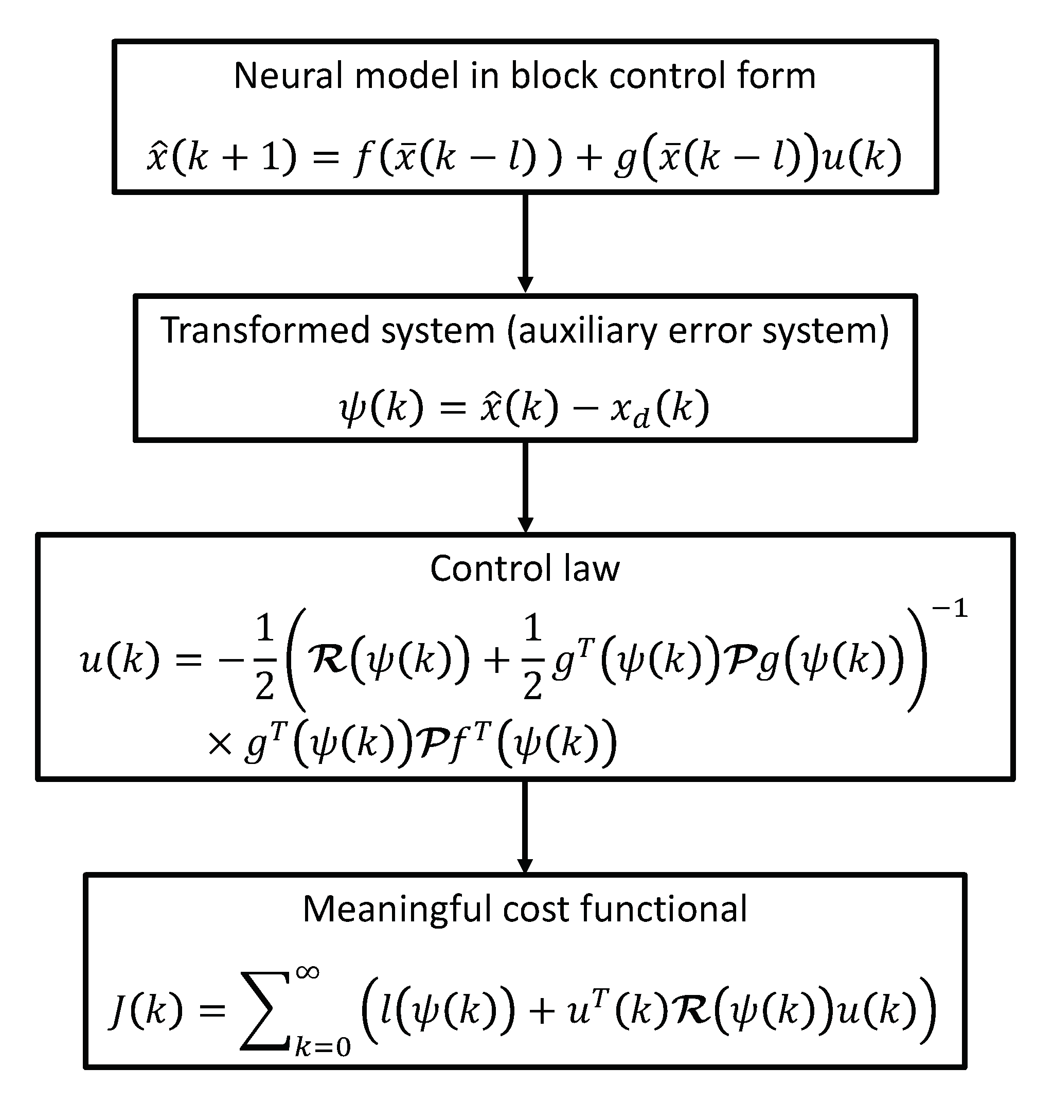
3.1. Neural Identification

As previously explained, the quantization error is a source of problems that can be encountered in real-time implementations. In almost all quantized output feedback control systems, quantization effects exist in the communication channel from sensor-to-controller, as well as from controller-to-actuator [17]. From now on, let us consider that the measured system signals and the controller output will be quantized before they are transmitted to the controller and the plant via a communication network.

However, it is necessary to consider that both measurement and actuator errors due to the unmodeled dynamics that appear in real-life problems; in this manner, an identification scheme can be represented as in Figure 1. Moreover, for unknown nonlinear systems with uncertainties, disturbances, and delays, a neural identifier can give an accurate model. System illustrated in Figure 1, can be modeled as:

$$\begin{array}{ccc}\hfill x_i\left(k+1\right)& =& f_i\left(\overline{x}\left(k-l\right)\right)+g_i\left(\overline{x}\left(k-l\right)\right)u\left(k\right)+d_i\left(k\right),i=1,\cdots ,n,\hfill \\ \hfill y\left(k\right)& =& Cx\left(k\right),\hfill \end{array}$$

(12)

where $\overline{x}$ is the quantized state, u represents the ideal calculated control law, l is the unknown delay for the state, and $d_i$ represents unknown disturbances. From Figure 1, it can be seen that a recurrent high order neural network (RHONN) is trained with quantized measured values of the state $\overline{x}$ and calculated values of the input u.

In this paper, the measured values of the state $\overline{x}$ are considered to be an unknown nonlinear function which depends on its quantized error $e_s$, delay l and time k, as follows:

$$\begin{array}{ccc}\hfill \overline{x}\left(k-l\right)& =& \delta \left(x_q\left(k\right),e_s\left(k\right),l,k\right)<\overline{\delta },\hfill \end{array}$$

with $\gamma$ an unknown function assumed bounded by $\overline{\gamma }$ which is also considered unknown; also, $x_q$ is defined as in (10). Then, we propose a neural identifier for the system (12), with the following structure:

$$\begin{array}{ccc}\hfill \widehat{x}\left(k\right)& =& {\left[\begin{array}{ccccc}{\widehat{x}}_1\left(k\right)& \dots & {\widehat{x}}_i\left(k\right)& \dots & {\widehat{x}}_n\left(k\right)\end{array}\right]}^{\top },\hfill \\ \hfill {\widehat{x}}_i(k+1)& =& w_i^{\top }{z}_i(\overline{x}\left(k-l\right),u\left(k\right)),\hfill \end{array}$$

(13)

with $z_i(\overline{x}\left(k-l\right),u\left(k\right))$ defined as

$$z_i(x\left(k\right),\varrho \left(k\right))=\left[\begin{array}{c}{z}_{i_1}\\ z_{i_2}\\ ⋮\\ z_{i_{L_i}}\end{array}\right]=\left[\begin{array}{c}{\Pi }_{j\in I_1}{\xi }_{i_j}^{d{i}_j\left(1\right)}\\ {\Pi }_{j\in I_2}{\xi }_{i_j}^{d_{ij}\left(2\right)}\\ ⋮\\ {\Pi }_{j\in I_{L_i}}{\xi }_{i_j}^{d{i}_j\left(L_i\right)}\end{array}\right],$$

(14)

with $d_{i_j}\left(k\right)$ being non-negative integers, and

$${\xi }_i=\left[\begin{array}{c}{\xi }_{i_1}\\ ⋮\\ {\xi }_{i_n}\\ {\xi }_{i_{n+1}}\\ ⋮\\ {\xi }_{i_{n+m}}\end{array}\right]=\left[\begin{array}{c}S\left({\overline{x}}_1\right)\\ ⋮\\ S\left({\overline{x}}_n\right)\\ u_1\left(k\right)\\ ⋮\\ u_m\left(k\right)\end{array}\right],$$

(15)

where $S(•)$ is defined as any sigmoid function as:

$$S\left(\varsigma \right)=\frac{1}{1+exp(-\beta \varsigma )},\beta >0,$$

(16)

and $\varsigma$ is any real valued variable.

As discussed in [24], the general discrete-time nonlinear system (1) can be approximated by a RHONN. In this paper the following discrete-time RHONN has been selected:

$$x\left(k+1\right)=w^{*\top }z\left(\overline{x}\left(k-l\right),u\left(k\right)\right)+{ϵ}_z,$$

(17)

and in the state component-wise form as

$$x_i\left(k+1\right)=w_i^{*\top }{z}_i\left(\overline{x}\left(k-l\right),u\left(k\right)\right)+{ϵ}_{z_i},i=1,\cdots ,n,$$

(18)

where $\overline{x}$ is the measured plant state, and ${ϵ}_{z_i}$ is a bounded approximation error, which can be reduced by increasing the number of the adjustable weights [24]. Let us assume that there exists an optimal weights vector $w_i^{*}\in {\Re }^{L_i}$, such that $∥{ϵ}_{z_i}∥$ is minimized on a compact set $w_{z_i}\subset {\Re }^{L_i}$ which is an artificial quantity required only for analytical purposes. In general, it is assumed that this optimal weight vector exists, and it is constant but unknown [24].

Let us define the estimate of $w_i^{*}$ as $w_i$; then, the weight estimation error ${\tilde{w}}_i\left(k\right)$ and identification error ${\tilde{x}}_i\left(k\right)$ are defined, respectively as

$${\tilde{w}}_i\left(k\right)=w_i^{*}-w_i\left(k\right),$$

(19)

and

$${\tilde{x}}_i\left(k\right)={\overline{x}}_i\left(k\right)-{\widehat{x}}_i\left(k\right).$$

(20)

The weight vectors are updated online with a decoupled extended Kalman filter (EKF) training algorithm, described by

$$\begin{array}{ccc}\hfill w_i\left(k+1\right)& =& w_i\left(k\right)+{\eta }_i\left(k\right)K_i\left(k\right){\tilde{x}}_i\left(k\right),\hfill \end{array}$$

(21)

$$\begin{array}{ccc}\hfill K_i\left(k\right)& =& P_i\left(k\right)H_i\left(k\right)M_i\left(k\right),\hfill \end{array}$$

(22)

$$\begin{array}{ccc}\hfill P_i\left(k+1\right)& =& P_i\left(k\right)-K_i\left(k\right)H_i^{\top }\left(k\right)P_i\left(k\right)+Q_i\left(k\right),\hfill \end{array}$$

(23)

with

$$\begin{array}{ccc}\hfill M_i\left(k\right)& =& {\left[R_i\left(k\right)+H_i^{\top }\left(k\right)P_i\left(k\right)H_i\left(k\right)\right]}^{-1},\hfill \\ \hfill i& =& 1,\cdots ,n,\hfill \end{array}$$

(24)

and the identification error is defined as in (20). The dynamics of $x_i\left(k+1\right)$ can be expressed as

$${\tilde{x}}_i\left(k+1\right)=x_i\left(k+1\right)-{\widehat{x}}_i\left(k+1\right)+e_{q{x}_i}\left(k\right),$$

(25)

with

$$e_{q{x}_i}\left(k\right)={\overline{x}}_i\left(k\right)-x_i\left(k\right),$$

(26)

as the state quantization error. From (10), this last equation can be rewritten as:

$$e_{q{x}_i}\left(k\right)={\mu }_x\left(q\left(\frac{x\left(k\right)}{{\mu }_x}\right)-\frac{x\left(k\right)}{{\mu }_x}\right).$$

(27)

To determine the state quantization error, first consider the property defined in (8), then,

$$\left|\frac{x\left(k\right)}{{\mu }_x}\right|\le M_x,$$

(28)

and

$$\left|q\left(\frac{x\left(k\right)}{{\mu }_x}\right)-\frac{x\left(k\right)}{{\mu }_x}\right|\le D_x,$$

(29)

By using the homogeneity property of the Euclidian norm, from (27) the following equation is obtained

$$\begin{array}{ccc}\left|e_{q{x}_i}\left(k\right)\right|\hfill & =& \left|{\mu }_x\left(q\left(\frac{x\left(k\right)}{{\mu }_x}\right)-\frac{x\left(k\right)}{{\mu }_x}\right)\right|\hfill \\ & =& {\mu }_x\left|\left(q\left(\frac{x\left(k\right)}{{\mu }_x}\right)-\frac{x\left(k\right)}{{\mu }_x}\right)\right|\le {\mu }_x{\Delta }_x.\hfill \end{array}$$

(30)

Considering the quantized system (18) and (13), the dynamics of (25) can be defined as:

$$\begin{array}{ccc}{\tilde{x}}_i\left(k+1\right)\hfill & =& x_i\left(k+1\right)-{\widehat{x}}_i\left(k+1\right)+e_{q{x}_i}\left(k\right)\hfill \\ & =& {\tilde{w}}_i^T\left(k\right)z_i\left(\overline{x}\left(k\right)\right)+{ϵ}_{z_i}+e_{q{x}_i}\left(k\right).\hfill \end{array}$$

(31)

By using (21), the weight estimation error dynamics (19) can be defined as:

$${\tilde{w}}_i\left(k+1\right)={\tilde{w}}_i\left(k\right)-{\eta }_i\left(k\right)K_i\left(k\right){\tilde{x}}_i\left(k\right).$$

(32)

Thus, considering (12), (31) and (32), then, it is possible to establish the following main result for an unknown nonlinear system with nonlinear output.

Theorem 2.

For a quantized delayed system (12), the neural identifier (13), trained with the EKF-based algorithm (21), ensures that the identification error (25) and the weight estimation error (32) are semi-globally uniformly ultimately bounded (SGUUB).

Proof of Theorem 2.

Step 1. For each element of $V\left(k\right)$, defined as $V_i\left(k\right)$ for $i=1,2,\cdots ,n$, let us consider the following Lyapunov function candidate:

$$V_i\left(k\right)={\gamma }_i{\left({\tilde{x}}_i\left(k\right)\right)}^2+{\tilde{w}}_i^T\left(k\right)P_i\left(k\right){\tilde{w}}_i\left(k\right).$$

(33)

Its first difference can be written as:

$$\begin{array}{ccc}\Delta V_i\left(k\right)\hfill & =& {\gamma }_i{\left({\tilde{x}}_i\left(k+1\right)\right)}^2+{\tilde{w}}_i^T\left(k+1\right)P_i\left(k+1\right){\tilde{w}}_i\left(k+1\right)-{\gamma }_i{\left({\tilde{x}}_i\left(k\right)\right)}^2\hfill \\ & & -{\tilde{w}}_i^T\left(k\right)P_i\left(k\right){\tilde{w}}_i\left(k\right).\hfill \end{array}$$

(34)

Substituting (31) and (32) in (34) it yields

$$\begin{array}{ccc}\Delta V_i\left(k\right)\hfill & =& {\gamma }_i{\left({\tilde{w}}_i^T\left(k\right)z_i\left(\overline{x}\left(k-l\right),u\left(k\right)\right)+{ϵ}_{z_i}+e_{q{x}_i}\left(k\right)\right)}^2\hfill \\ & & +{\left({\tilde{w}}_i\left(k\right)-{\eta }_i\left(k\right)K_i\left(k\right){\tilde{x}}_i\left(k\right)\right)}^T\left(P_i\left(k\right)-A_i\left(k\right)\right)\hfill \\ & & \times \left({\tilde{w}}_i\left(k\right)-{\eta }_i\left(k\right)K_i\left(k\right){\tilde{x}}_i\left(k\right)\right)-{\gamma }_i{\left({\tilde{x}}_i\left(k\right)\right)}^2-{\tilde{w}}_i^T\left(k\right)P_i\left(k\right){\tilde{w}}_i\left(k\right).\hfill \end{array}$$

Then,

$$\begin{array}{ccc}\Delta V_i\left(k\right)\hfill & =& {\gamma }_i{\left({\tilde{w}}_i^T\left(k\right)z_i\left(\overline{x}\left(k-l\right),u\left(k\right)\right)\right)}^2-{\tilde{w}}_i^T\left(k\right)A_i\left(k\right){\tilde{w}}_i\left(k\right)\hfill \\ & & +{\eta }_i^2\left(k\right){\tilde{x}}_i^T\left(k\right)K_i^T\left(k\right)P_i\left(k\right)K_i\left(k\right){\tilde{x}}_i\left(k\right)-{\gamma }_i{\left({\tilde{x}}_i\left(k\right)\right)}^2\hfill \\ & & -{\eta }_i\left(k\right){\tilde{x}}_i^T\left(k\right)K_i^T\left(k\right)A_i\left(k\right){\tilde{x}}_i\left(k\right)+2{\gamma }_i{\tilde{w}}_i^T\left(k\right)z_i\left(\overline{x}\left(k-l\right),u\left(k\right)\right){ϵ}_{z_i}\hfill \\ & & +2{\gamma }_i{\tilde{w}}_i^T\left(k\right)z_i\left(\overline{x}\left(k-l\right),u\left(k\right)\right)e_{q{x}_i}\left(k\right)-{\eta }_i\left(k\right){\tilde{w}}_i^T\left(k\right)P_i\left(k\right)K_i\left(k\right){\tilde{x}}_i\left(k\right)\hfill \\ & & +{\tilde{w}}_i^T\left(k\right)A_i\left(k\right){\tilde{x}}_i\left(k\right)-{\eta }_i\left(k\right){\tilde{x}}_i^T\left(k\right)K_i^T\left(k\right)P_i\left(k\right){\tilde{w}}_i\left(k\right)\hfill \\ & & +{\eta }_i\left(k\right){\tilde{x}}_i^T\left(k\right)K_i^T\left(k\right)A_i\left(k\right){\tilde{w}}_i\left(k\right)+{\gamma }_i{ϵ}_{z_i}^2+2{\gamma }_i{ϵ}_{z_i}{e}_{q{x}_i}\left(k\right)+{\gamma }_i{e}_{q{x}_i}^2\left(k\right).\hfill \end{array}$$

with $A_i\left(k\right)=K_i\left(k\right)H_i^{\top }\left(k\right)P_i\left(k\right)-Q_i\left(k\right)$. Now, using the following inequalities

$$\begin{array}{ccc}\hfill X^{T}X+Y^{T}Y& \ge & 2X^{T}Y,\hfill \\ \hfill X^{T}X+Y^{T}Y& \ge & -2X^{T}Y,\hfill \\ \hfill -{\lambda }_{min}\left(P\right)\left(X^{T}X\right)& \ge & -X^{T}PX\ge -{\lambda }_{max}\left(P\right)\left(X^{T}X\right),\hfill \end{array}$$

(35)

which are valid $\forall X,Y\in {\Re }^n$ with $\forall P\in {\Re }^{n\times n},$ $P=P^T>0$, using (35), then $\Delta V_i\left(k\right)$ can be rewritten as

$$\begin{array}{ccc}\Delta V_i\left(k\right)\hfill & \le & {\gamma }_i{\left({\tilde{w}}_i^T\left(k\right)z_i\left(\overline{x}\left(k-l\right),\overline{u}\left(k\right)\right)\right)}^2-{\tilde{w}}_i^T\left(k\right)A_i\left(k\right){\tilde{w}}_i\left(k\right)\hfill \\ & & +{\eta }_i^2\left(k\right){\tilde{x}}_i^T\left(k\right)K_i^T\left(k\right)P_i\left(k\right)K_i\left(k\right){\tilde{x}}_i\left(k\right)-{\gamma }_i{\left({\tilde{x}}_i\left(k\right)\right)}^2\hfill \\ & & -{\eta }_i\left(k\right){\tilde{x}}_i^T\left(k\right)K_i^T\left(k\right)A_i\left(k\right){\tilde{x}}_i\left(k\right)+4{\gamma }_i{\left({\tilde{w}}_i^T\left(k\right)z_i\left(\overline{x}\left(k-l\right),u\left(k\right)\right)\right)}^2+{ϵ}_{z_i}^2\hfill \\ & & +4{\gamma }_i{\left({\tilde{w}}_i^T\left(k\right)z_i\left(\overline{x}\left(k-l\right),u\left(k\right)\right)\right)}^2+e_{q{x}_i}^2\left(k\right)+{\eta }_i^2\left(k\right){\tilde{x}}_i^T\left(k\right)K_i^T\left(k\right)K_i\left(k\right){\tilde{x}}_i\left(k\right)\hfill \\ & & +A_i\left(k\right){\tilde{w}}_i\left(k\right){\tilde{w}}_i^T\left(k\right)A_i\left(k\right)+{\eta }_i^2\left(k\right){\tilde{w}}_i^T\left(k\right)P_i\left(k\right)P_i^T\left(k\right){\tilde{w}}_i\left(k\right)\hfill \\ & & +K_i\left(k\right){\tilde{x}}_i\left(k\right){\tilde{x}}_i^T\left(k\right)K_i^T\left(k\right)+{\tilde{w}}_i^T\left(k\right)A_i\left(k\right)A_i^T\left(k\right){\tilde{w}}_i\left(k\right)\hfill \\ & & +{\tilde{x}}_i\left(k\right){\tilde{x}}_i^T\left(k\right)+{\eta }_i^2\left(k\right){\tilde{x}}_i^T\left(k\right)K_i^T\left(k\right)K_i\left(k\right){\tilde{x}}_i\left(k\right)\hfill \\ & & +P_i\left(k\right){\tilde{w}}_i\left(k\right){\tilde{w}}_i^T\left(k\right)P_i\left(k\right)+{\gamma }_i{ϵ}_{z_i}^2+2{\gamma }_i{ϵ}_{z_i}{e}_{q{x}_i}\left(k\right)+{\gamma }_i{e}_{q{x}_i}^2\left(k\right).\hfill \end{array}$$

Then,

$$\begin{array}{ccc}\Delta V_i\left(k\right)\hfill & \le & {\gamma }_i{∥{\tilde{w}}_i\left(k\right)∥}^2{∥z_i\left(\overline{x}\left(k-l\right),u\left(k\right)\right)∥}^2-{∥{\tilde{w}}_i\left(k\right)∥}^2{\lambda }_{min}\left(A_i\left(k\right)\right)\hfill \\ & & -{\gamma }_i{∥{\tilde{x}}_i\left(k\right)∥}^2+{\eta }_i^2\left(k\right){∥{\tilde{x}}_i\left(k\right)∥}^2{∥K_i\left(k\right)∥}^2{\lambda }_{max}\left(P_i\left(k\right)\right)\hfill \\ & & -{\eta }_i\left(k\right){∥{\tilde{x}}_i\left(k\right)∥}^2{\lambda }_{min}\left(K_i\left(k\right)\right){\lambda }_{min}\left(A_i\left(k\right)\right)\hfill \\ & & +8{\gamma }_i^2{∥{\tilde{w}}_i\left(k\right)∥}^2{∥z_i\left(\overline{x}\left(k-l\right),u\left(k\right)\right)∥}^2+{\left|{ϵ}_{z_i}\right|}^2\hfill \\ & & +{\left|e_{q{x}_i}\left(k\right)\right|}^2+{\eta }_i^2\left(k\right){∥{\tilde{x}}_i\left(k\right)∥}^2{∥K_i\left(k\right)∥}^2+{∥A_i\left(k\right)∥}^2{∥{\tilde{w}}_i\left(k\right)∥}^2\hfill \\ & & +{\eta }_i^2\left(k\right){∥{\tilde{w}}_i\left(k\right)∥}^2{∥P_i\left(k\right)∥}^2+{∥K_i\left(k\right)∥}^2{∥{\tilde{x}}_i\left(k\right)∥}^2\hfill \\ & & +{∥{\tilde{w}}_i\left(k\right)∥}^2{∥A_i\left(k\right)∥}^2+{∥{\tilde{x}}_i\left(k\right)∥}^2+{\eta }_i^2\left(k\right){∥{\tilde{x}}_i\left(k\right)∥}^2{∥K_i\left(k\right)∥}^2\hfill \\ & & +{∥{\tilde{w}}_i\left(k\right)∥}^2{∥P_i\left(k\right)∥}^2+{\gamma }_i{\left|{ϵ}_{z_i}\right|}^2+2{\gamma }_i\left|{ϵ}_{z_i}\right|\left|e_{q{x}_i}\left(k\right)\right|+{\gamma }_i{\left|e_{q{x}_i}\left(k\right)\right|}^2.\hfill \end{array}$$

(36)

Defining

$$\begin{array}{ccc}{E}_i\left(k\right)\hfill & =& -{\gamma }_i{∥z_i\left(\overline{x}\left(k-l\right),u\left(k\right)\right)∥}^2+{\lambda }_{min}\left(A_i\left(k\right)\right)-8{\gamma }_i^2{∥z_i\left(\overline{x}\left(k-l\right),u\left(k\right)\right)∥}^2\hfill \\ & & -2{∥A_i\left(k\right)∥}^2-{\eta }_i^2\left(k\right){∥P_i\left(k\right)∥}^2-{∥P_i\left(k\right)∥}^2,\hfill \\ F_i\left(k\right)\hfill & =& -{\eta }_i^2\left(k\right){∥K_i\left(k\right)∥}^2{\lambda }_{max}\left(P_i\left(k\right)\right)+{\gamma }_i+{\eta }_i\left(k\right){\lambda }_{min}\left(K_i\left(k\right)\right){\lambda }_{min}\left(A_i\left(k\right)\right)\hfill \\ & & -2{\eta }_i^2\left(k\right){∥K_i\left(k\right)∥}^2-{∥K_i\left(k\right)∥}^2-1,\hfill \end{array}$$

and selecting ${\gamma }_i$, ${\eta }_i$, $Q_i$ and $R_i$ such that $E_i>0$ and $F_i>0$, $\forall k$, then (36) can be expressed as:

$$\begin{array}{ccc}\Delta V_i\left(k\right)\hfill & =& -{∥{\tilde{w}}_i\left(k\right)∥}^2{E}_i\left(k\right)-{∥{\tilde{x}}_i\left(k\right)∥}^2{F}_i\left(k\right)+{\left|{ϵ}_{z_i}\right|}^2+{\left|D_{x_i}\right|}^2+{\gamma }_i{\left|{ϵ}_{z_i}\right|}^2\hfill \\ & & +2{\gamma }_i\left|{ϵ}_{z_i}\right|\left|D_{x_i}\right|+{\gamma }_i{\left|D_{x_i}\right|}^2,\hfill \end{array}$$

(37)

with $\left|e_{q{x}_i}\left(k\right)\right|\le {\mu }_x{D}_x$ from (30). Then, $\Delta V_i\left(k\right)<0$ when

$$∥{\tilde{w}}_i\left(k\right)∥>\sqrt{\frac{{\left|{ϵ}_{z_i}\right|}^2+{\left|{\Delta }_{x_i}\right|}^2+{\gamma }_i{\left|{ϵ}_{z_i}\right|}^2+2{\gamma }_i\left|{ϵ}_{z_i}\right|\left|{\Delta }_{x_i}\right|+{\gamma }_i{\left|{\Delta }_{x_i}\right|}^2}{E_i\left(k\right)}}\equiv {\kappa }_1\left(k\right),$$

(38)

or

$$∥{\tilde{x}}_i\left(k\right)∥>\sqrt{\frac{{\left|{ϵ}_{z_i}\right|}^2+{\left|{\Delta }_{x_i}\right|}^2+{\gamma }_i{\left|{ϵ}_{z_i}\right|}^2+2{\gamma }_i\left|{ϵ}_{z_i}\right|\left|{\Delta }_{x_i}\right|+{\gamma }_i{\left|{\Delta }_{x_i}\right|}^2}{F_i\left(k\right)}}\equiv {\kappa }_2\left(k\right).$$

(39)

Step 2. Now, for $V\left(k\right)$, consider the Lyapunov function candidate

$$V\left(k\right)=\sum _{i=1}^n\left({\gamma }_i{\left({\tilde{x}}_i\left(k\right)\right)}^2+{\tilde{w}}_i^T\left(k\right)P_i\left(k\right){\tilde{w}}_i\left(k\right)\right).$$

(40)

Its first difference can be written as:

$$\begin{array}{ccc}\Delta V\left(k\right)\hfill & =& \sum _{i=1}^n\left({\gamma }_i{\left({\tilde{x}}_i\left(k+1\right)\right)}^2+{\tilde{w}}_i^T\left(k+1\right)P_i\left(k+1\right){\tilde{w}}_i\left(k+1\right)\right.\hfill \\ & & \left.-{\gamma }_i{\left({\tilde{x}}_i\left(k\right)\right)}^2-{\tilde{w}}_i^T\left(k\right)P_i\left(k\right){\tilde{w}}_i\left(k\right)\right).\hfill \end{array}$$

(41)

Substituting (31) and (32) in (41) yields

$$\begin{array}{ccc}\Delta V\left(k\right)\hfill & =& \sum _{i=1}^n\left({\gamma }_i{\left({\tilde{w}}_i^T\left(k\right)z_i\left(\overline{x}\left(k-l\right),u\left(k\right)\right)+{ϵ}_{z_i}+e_{q{x}_i}\left(k\right)\right)}^2\right.\hfill \\ & & +{\left({\tilde{w}}_i\left(k\right)-{\eta }_i\left(k\right)K_i\left(k\right){\tilde{x}}_i\left(k\right)\right)}^T\left(P_i\left(k\right)-A_i\left(k\right)\right)\hfill \\ & & \times \left({\tilde{w}}_i\left(k\right)-{\eta }_i\left(k\right)K_i\left(k\right){\tilde{x}}_i\left(k\right)\right)\hfill \\ & & \left.-{\gamma }_i{\left({\tilde{x}}_i\left(k\right)\right)}^2-{\tilde{w}}_i^T\left(k\right)P_i\left(k\right){\tilde{w}}_i\left(k\right)\right).\hfill \end{array}$$

(42)

Defining

$$\begin{array}{ccc}{A}_i\left(k\right)\hfill & =& K_i\left(k\right)H_i^{\top }\left(k\right)P_i\left(k\right)-Q_i\left(k\right),\hfill \\ E_i\left(k\right)\hfill & =& -{\gamma }_i{∥z_i\left(\overline{x}\left(k-l\right),u\left(k\right)\right)∥}^2+{\lambda }_{min}\left(A_i\left(k\right)\right)-8{\gamma }_i^2{∥z_i\left(\overline{x}\left(k-l\right),u\left(k\right)\right)∥}^2\hfill \\ & & -2{∥A_i\left(k\right)∥}^2-{\eta }_i^2\left(k\right){∥P_i\left(k\right)∥}^2-{∥P_i\left(k\right)∥}^2,\hfill \\ F_i\left(k\right)\hfill & =& -{\eta }_i^2\left(k\right){∥K_i\left(k\right)∥}^2{\lambda }_{max}\left(P_i\left(k\right)\right)+{\gamma }_i+{\eta }_i\left(k\right){\lambda }_{min}\left(K_i\left(k\right)\right){\lambda }_{min}\left(A_i\left(k\right)\right)\hfill \\ & & -2{\eta }_i^2\left(k\right){∥K_i\left(k\right)∥}^2-{∥K_i\left(k\right)∥}^2-1,\hfill \end{array}$$

and selecting ${\gamma }_i$, ${\eta }_i$, $Q_i$ and $R_i$ such that $E_i>0$ and $F_i>0$, $\forall k$, then (42) can be expressed as:

$$\begin{array}{ccc}\Delta V_i\left(k\right)\hfill & =& \sum _{i=1}^n\left(-{∥{\tilde{w}}_i\left(k\right)∥}^2{E}_i\left(k\right)-{∥{\tilde{x}}_i\left(k\right)∥}^2{F}_i\left(k\right)+{\left|{ϵ}_{z_i}\right|}^2+{\left|{\Delta }_{x_i}\right|}^2\right.\hfill \\ & & \left.+{\gamma }_i{\left|{ϵ}_{z_i}\right|}^2+2{\gamma }_i\left|{ϵ}_{z_i}\right|\left|{\Delta }_{x_i}\right|+{\gamma }_i{\left|{\Delta }_{x_i}\right|}^2\right).\hfill \end{array}$$

(43)

Then, $\Delta V_i\left(k\right)<0$ when (38) and (39) is fulfilled for $i=1,2,\cdots ,n$. Therefore, considering Step 1 and Step 2 for (40), the solution of (31) and (32) is SGUUB.  □

Remark 1.

Considering Theorem 2 and its proof, it can be demonstrated that the result can be extended for systems with multiple delays such as $x\left(k-l_i\right)$ with $i=1,2,\cdots$ used instead of $x(k-l)$ in (1), and for systems with time-varying delays $x(k-l_i\left(k\right))$ with $l_i\left(k\right)$ bounded by $l_i\left(k\right)\le l_i$ in such case $x(k-l_i\left(k\right))$ can be substituted by $x\left(k-l_i\right)$ and can be handled as in previous proof due to the boundedness of RHONN. Also, from (43) it can be seen that RHONN (38) can identify a quantized discrete-time unknown delayed nonlinear system, this neural model can be arbitrarily designed in an affine form in order to deal with control goals.

3.2. Neural Inverse Optimal Control

In the previous section, a neural identifier has been designed for a quantized discrete-time unknown delayed nonlinear system under disturbances and uncertainties; all these phenomena are now modeled by the neural identifier (13) without the need to measure or estimate or even know their boundaries. In this section, the obtained neural model is used to design a controller for such systems, using the inverse optimality methodology, a controller for the system is designed.

Then, considering Theorem 1 and Theorem 2, it is possible to establish the following main result, for the closed-loop system:

Theorem 3.

Consider a control law (5) for a quantized delayed system (12) modeled by a RHONN (13), trained with an EKF (21), ensuring that the identification error (31) and the trajectory tracking error (3) are SGUUB; moreover, the RHONN weight (32) remain bounded.

Proof. 

Consider the following augmented Lyapunov function candidate

$$\mathcal{V}\left(k\right)={\mathcal{V}}_1\left(k\right)+{\mathcal{V}}_2\left(k\right),$$

(44)

with

$$\begin{array}{ccc}\hfill {\mathcal{V}}_1\left(k\right)& =& \sum _{i=1}^n\left({\Gamma }_i{\left({\tilde{x}}_i\left(k\right)\right)}^2+{\tilde{w}}_i^T\left(k\right)P_i\left(k\right){\tilde{w}}_i\left(k\right)\right),\hfill \end{array}$$

(45)

$$\begin{array}{ccc}\hfill {\mathcal{V}}_2\left(k\right)& =& \frac{1}{2}{\psi }^T\left(k\right)\mathcal{P}\psi \left(k\right).\hfill \end{array}$$

(46)

The first difference from (44) results

$$\begin{array}{ccc}\Delta \mathcal{V}\left(k\right)\hfill & =& {\mathcal{V}}_1\left(k+1\right)-{\mathcal{V}}_1\left(k\right)+{\mathcal{V}}_2\left(k+1\right)-{\mathcal{V}}_2\left(k\right)\hfill \\ & =& \sum _{i=1}^n\left({\Gamma }_i{\left({\tilde{x}}_i\left(k+1\right)\right)}^2+{\tilde{w}}_i^T\left(k+1\right)P_i\left(k\right){\tilde{w}}_i\left(k+1\right)\right)\hfill \\ & & -\sum _{i=1}^n\left({\Gamma }_i{\left({\tilde{x}}_i\left(k\right)\right)}^2+{\tilde{w}}_i^T\left(k\right)P_i\left(k\right){\tilde{w}}_i\left(k\right)\right)\hfill \\ & & +\frac{1}{2}{\psi }^T\left(k+1\right)\mathcal{P}\psi \left(k+1\right)-\frac{1}{2}{\psi }^T\left(k\right)\mathcal{P}\psi \left(k\right).\hfill \end{array}$$

(47)

Case 1. For $\Delta {\mathcal{V}}_1\left(k\right)$. From Theorem 2, (47) can be expressed as:

$$\begin{array}{ccc}\Delta {\mathcal{V}}_1\left(k\right)\hfill & =& \sum _{i=1}^n\left(-{∥{\tilde{w}}_i\left(k\right)∥}^2{E}_i\left(k\right)-{∥{\tilde{x}}_i\left(k\right)∥}^2{F}_i\left(k\right)+{\left|{ϵ}_{z_{iu}}\right|}^2+{\left|{\Delta }_{x_i}\right|}^2\right.\hfill \\ & & \left.+{\Gamma }_i{\left|{ϵ}_{z_{iu}}\right|}^2+2{\Gamma }_i\left|{ϵ}_{z_{iu}}\right|\left|{\Delta }_{x_i}\right|+{\Gamma }_i{\left|{\Delta }_{x_i}\right|}^2\right).\hfill \end{array}$$

(48)

Then, $\Delta {\mathcal{V}}_1\left(k\right)<0$ when (38) and (39) is fulfilled for $i=1,2,\cdots ,n$.

Case 2. For $\Delta {\mathcal{V}}_2\left(k\right)$. Consider (1) and (3), then

$$\begin{array}{ccc}\Delta {\mathcal{V}}_2\left(k\right)\hfill & =& \frac{1}{2}{f}^T\left(\psi \left(k\right)\right)\mathcal{P}f\left(\psi \left(k\right)\right)+\frac{1}{2}{f}^T\left(\psi \left(k\right)\right)\mathcal{P}g\left(\psi \left(k\right)\right)u\left(k\right)\hfill \\ & & +\frac{1}{2}{u}^T\left(k\right)g^T\left(\psi \left(k\right)\right)\mathcal{P}f\left(\psi \left(k\right)\right)+\frac{1}{2}{u}^T\left(k\right)g^T\left(\psi \left(k\right)\right)\mathcal{P}g\left(\psi \left(k\right)\right)u\left(k\right)\hfill \\ & & -\frac{1}{2}{\psi }^T\left(k\right)\mathcal{P}\psi \left(k\right),\hfill \end{array}$$

(49)

with (5). From Theorem 1 [23], $\Delta {\mathcal{V}}_2\left(k\right)\le -{\psi }^T\left(k\right)\mathcal{Q}\psi \left(k\right)$ with $\mathcal{Q}={\mathcal{Q}}^T>0.$ Therefore, considering Case 1 and Case 2, for (44), the solutions of (25), (32) and (3) are SGUUB.  □

The entire closed-loop system is depicted in Figure 2. Theorem 3 ensures the stability of the closed-loop system, without the assumption of persistent excitation. It is necessary to point out that the inverse optimal controller is designed for the neural model not for the system model, which is considered unknown. This means that the neural model considers system dynamics, sensor errors, actuators errors, disturbances, uncertainties, and unmodeled dynamics.

Remark 2.

It is important to note that in this paper, the unknown discrete-time quantized delayed system (12) is modeled by a RHONN (13), trained with an EKF learning algorithm (21), then the controller is designed based on the RHONN model. Therefore, the RHONN model (13) is designed in order that the controllable block form required by the controller (5) can be easily obtained in the required affine form. Furthermore, controllability weights of RHONN model (13) are selected as fixed weights to avoid singularities due to controller feedback [23].

Remark 3.

As explained in Section 3.2 any nonlinear trajectory tracking problem can be transformed into an error regulation problem [9]; this transformation is displayed in Figure 3 including the design of a neural inverse optimal control (NIOC).

4. Real-Time Results

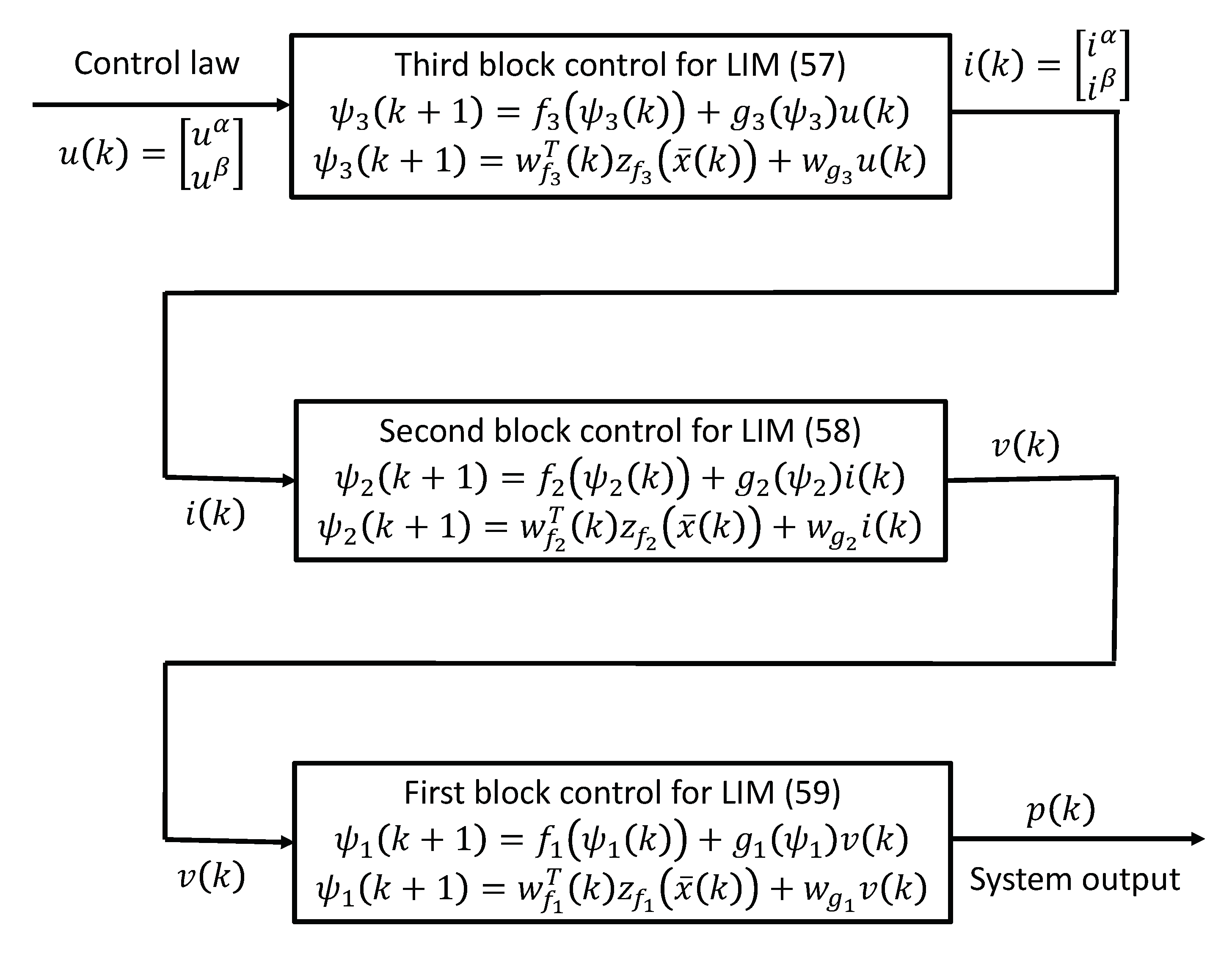
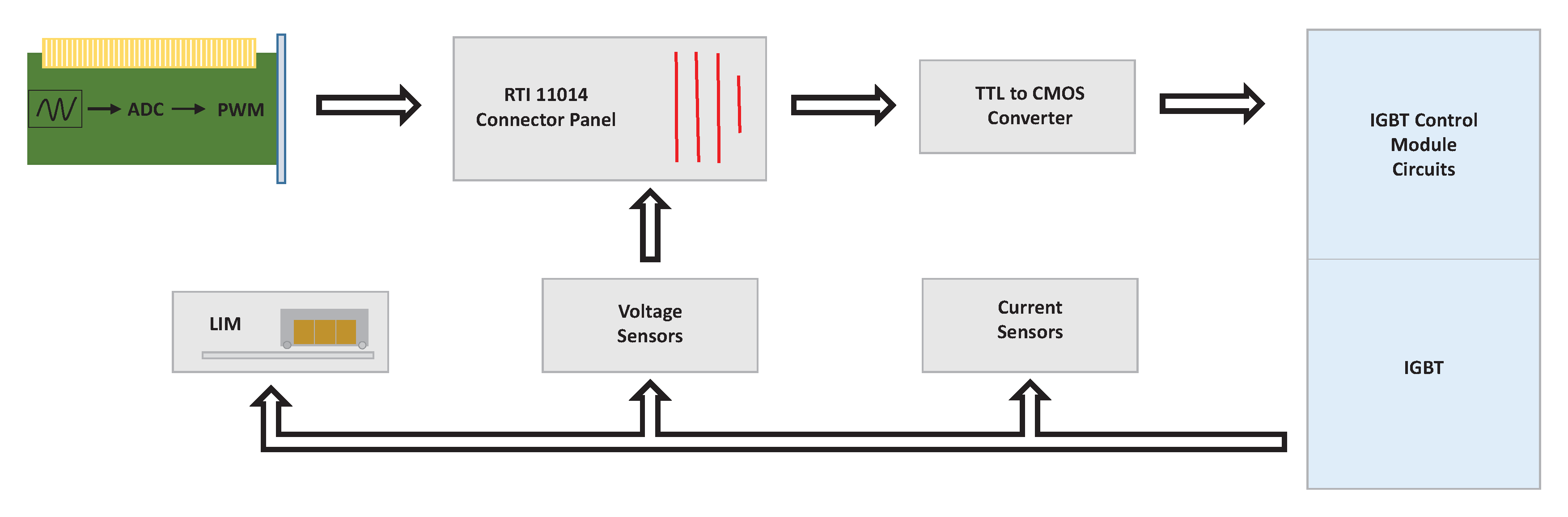
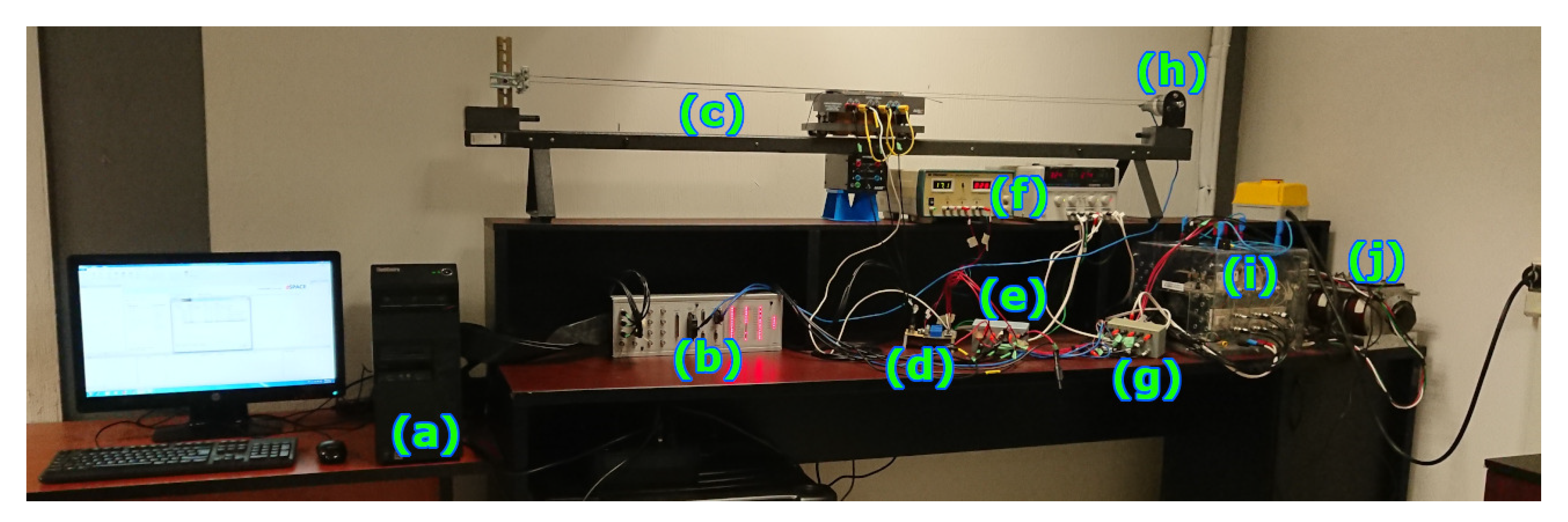
4.1. Implementation to a LIM

In this section, a NIOC scheme is designed to be implemented in a linear induction motor (LIM) prototype in the presence of all the phenomena, as mentioned earlier. First, a neural identifier is designed for the LIM system, considering an unknown model with disturbances, uncertainties, quantization in measured signals, measurement noise, and delays. Therefore, the obtained neural state model is used to design a controller for the LIM using the inverse optimal methodology considering actuator limitations.

A LIM is an electrical machine in which electrical energy is directly transformed into mechanical energy as a translational movement. LIMs have excellent performance characteristics [25,26], such as high-starting thrust force, elimination of gears between motor and motion devices, reduction of mechanical losses and size of motion devices, high-speed operation, silent operation, among others. The driving principles of a LIM are similar to the ones of a traditional rotary induction motor. However, the LIM mathematical model is more complicated; its control design is also a complex task due to the exceedingly time-varying nature of its parameters. This is due to the change of operating conditions, such as speed, temperature, and rail configuration, to name a few. LIMs have been used for mass public transportation, 3D printing, material transportation, elevators, aircraft carrier, industrial processes, automation, and home appliances, among others [25].

From previous works, it is possible to remark that in [22], a neural inverse optimal controller has been proposed for a LIM; however, such controller only considers disturbances meanwhile delays are disregarded. Also, a neural identifier for a LIM is proposed in [1]. Then, in [2], time delays are considered as well as disturbances, with a sliding mode neural controller for the same system. Nonetheless, none of the above-referenced works include real-time implementation of the controller when simultaneously considering, disturbances, noise, delays, actuator limitations, and quantization for a system with an unknown model. Therefore, in this section, the design of a neural controller for a LIM is proposed. Such a controller considers all the phenomena mentioned earlier while intending to control complex systems with conditions increasingly closer to that of real-time experimentation.

4.2. NIOC Scheme

4.2.1. RHONN Model

The $\alpha -\beta$ mathematical model for a LIM is represented by the state vector (50), which includes position, velocity, flux magnitude, $\alpha$ current, and $\beta$ current. The control law vector $u\left(k\right)$ to be designed using the NIOC algorithm, given by (51), and its entries, namely $u_{\alpha }\left(k\right)$ and $u_{\beta }\left(k\right)$, represent the $\alpha$ and $\beta$ components, of the input voltage applied to the LIM, respectively.

$$\begin{array}{ccc}\hfill x\left(k\right)& =& \left[\begin{array}{c}{x}_1\left(k\right)\\ x_2\left(k\right)\\ x_3\left(k\right)\\ x_4\left(k\right)\\ x_5\left(k\right)\end{array}\right]=\left[\begin{array}{c}p\left(k\right)\\ v\left(k\right)\\ \psi \left(k\right)\\ i_{\alpha }\left(k\right)\\ i_{\beta }\left(k\right)\end{array}\right],\hfill \end{array}$$

(50)

$$\begin{array}{ccc}\hfill u\left(k\right)& =& \left[\begin{array}{c}{u}_{\alpha }\left(k\right)\\ u_{\beta }\left(k\right)\end{array}\right].\hfill \end{array}$$

(51)

For the design of the proposed RHONN identifier, which is given through (53), the state variables $x_1$, $x_2$, $x_4$ and $x_5$ are considered as measurable signals, and $\mathsf{\Psi }\left(k\right)=f_{\alpha }{\left(k\right)}^2+f_{\beta }{\left(k\right)}^2$ where $f_{\alpha }$ and $f_{\beta }$ are the $\alpha$ and $\beta$ flux components, respectively, estimated by a nonlinear observer [22]. The function $S\left(\upsilon \right)$ is defined as (54), and the identifier’s state variables are defined as:

$$\begin{array}{ccc}\hfill \widehat{x}\left(k\right)& =& \left[\begin{array}{c}{\widehat{x}}_1\left(k\right)\\ {\widehat{x}}_2\left(k\right)\\ {\widehat{x}}_3\left(k\right)\\ {\widehat{x}}_4\left(k\right)\\ {\widehat{x}}_5\left(k\right)\end{array}\right]=\left[\begin{array}{c}\widehat{p}\left(k\right)\\ \widehat{v}\left(k\right)\\ \widehat{\psi }\left(k\right)\\ {\widehat{i}}_{\alpha }\left(k\right)\\ {\widehat{i}}_{\beta }\left(k\right)\end{array}\right].\hfill \end{array}$$

(52)

For the identifier in (53), the quantized fluxes ${\overline{f}}_{\alpha }$ and ${\overline{f}}_{\beta }$, are not considered since the implemented prototype shown in Figure 4 cannot measure magnetic fluxes. As mentioned before, these variables are estimated by a reduced-order state-observer [22]. Also, the following weights are fixed: $w_f=0.001$, $w_{12}=0.001$, $w_{24}=0.001$, $w_{25}=0.001$, $w_{45}=0.05$, $w_{55}=0.05$ for controllability purposes, these values have been obtained heuristically in order to improve identification performance [27], neural identification accuracy is obtained due to the adaptable weight connections of the neural network another solution is the zero-crossing avoidance studied in [28]; the remaining weight vectors $w_i$ from the identifier in (53) are trained online by the EKF training algorithm in (21), with the parameters shown in

Table 1. EKF training parameters.

i	$\mathit{\eta }$	P	Q	R
$w_1$	$0.5$	2	$0.63759$	$0.0061914$
$w_2$	$0.5$	$2\times I_{3\times 3}$	$0.0067168\times I_{3\times 3}$	$0.0061914$
$w_3$	$0.5$	$2\times I_{3\times 3}$	$0.0067168\times I_{3\times 3}$	$0.0061914$
$w_4$	$0.5$	$2\times I_{4\times 4}$	$0.0045569\times I_{4\times 4}$	$0.0061914$
$w_5$	$0.5$	$2\times I_{4\times 4}$	$0.0045569\times I_{4\times 4}$	$0.0061914$

.

$$\begin{array}{ccc}\hfill {\widehat{x}}_1\left(k+1\right)& =& w_{11}\left(k\right)S\left(\overline{p}\left(k-l\right)\right)+w_{12}\overline{v}\left(k-l\right),\hfill \\ \hfill {\widehat{x}}_2\left(k+1\right)& =& w_{21}\left(k\right)S\left(\overline{v}\left(k-l\right)\right)+w_{22}\left(k\right)S\left({\psi }_{\alpha }\left(k-l\right)\right)+w_{23}\left(k\right)S\left({\psi }_{\beta }\left(k-l\right)\right)\hfill \\ \hfill & & -w_{24}\left(S\left({\psi }_{\alpha }\left(k-l\right)\right)+S\left({\psi }_{\beta }\left(k-l\right)\right)\right){\overline{i}}_{\alpha }\hfill \\ \hfill & & +w_{25}\left(S\left({\psi }_{\alpha }\left(k-l\right)\right)+S\left({\psi }_{\beta }\left(k-l\right)\right)\right){\overline{i}}_{\beta },\hfill \\ \hfill {\widehat{x}}_3\left(k+1\right)& =& w_{31}\left(k\right)S{\left({\psi }_{\alpha }\left(k-l\right)\right)}^2+w_{32}\left(k\right)S{\left({\psi }_{\beta }\left(k-l\right)\right)}^2\hfill \\ \hfill & & +w_{33}\left(k\right)w_{f}S{\left(\overline{v}\left(k-l\right)\right)}^2\hfill \\ \hfill & & +2w_f\left(w_{31}\left(k\right)S\left({\psi }_{\alpha }\left(k-l\right)\right)-w_{32}\left(k\right)S\left({\psi }_{\beta }\left(k-l\right)\right)\right){\overline{i}}_{\alpha }\left(k-l\right)\hfill \\ \hfill & & +2w_f\left(w_{31}\left(k\right)S\left({\psi }_{\alpha }\left(k-l\right)\right)+w_{32}\left(k\right)S\left({\psi }_{\beta }\left(k-l\right)\right)\right){\overline{i}}_{\beta }\left(k-l\right),\hfill \\ \hfill {\widehat{x}}_4\left(k+1\right)& =& w_{41}\left(k\right)S\left(\overline{v}\left(k-l\right)\right)+w_{42}\left(k\right)S\left({\psi }_{\alpha }\left(k-l\right)\right)+w_{43}\left(k\right)S\left({\psi }_{\beta }\left(k-l\right)\right)\hfill \\ \hfill & & +w_{44}\left(k\right)S\left({\overline{i}}_{\alpha }\left(k-l\right)\right)+w_{45}{u}_{\alpha }\left(k\right),\hfill \\ \hfill {\widehat{x}}_5\left(k+1\right)& =& w_{51}\left(k\right)S\left(\overline{v}\left(k-l\right)\right)+w_{52}\left(k\right)S\left({\psi }_{\alpha }\left(k-l\right)\right)+w_{53}\left(k\right)S\left({\psi }_{\beta }\left(k-l\right)\right)\hfill \\ \hfill & & +w_{54}\left(k\right)S\left({\overline{i}}_{\beta }\left(k-l\right)\right)+w_{55}{u}_{\beta }\left(k\right),\hfill \end{array}$$

(53)

$$S\left(\upsilon \right)=tanh\left(\upsilon \right).$$

(54)

4.2.2. Inverse Optimal Control

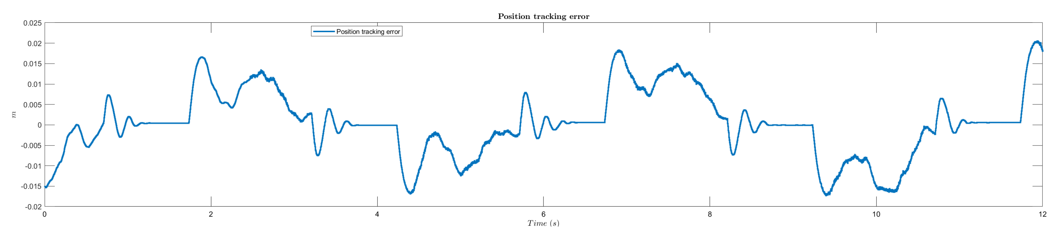
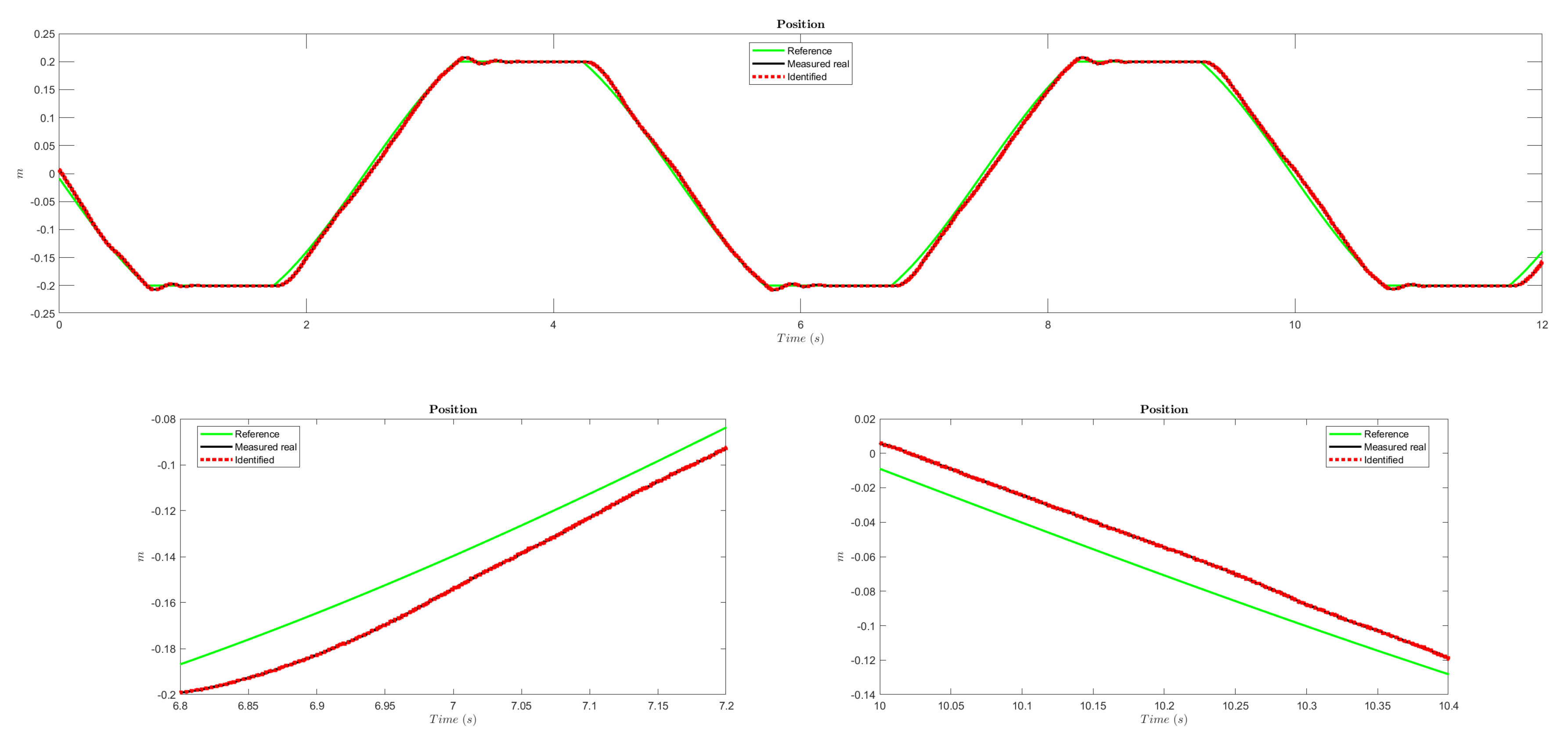
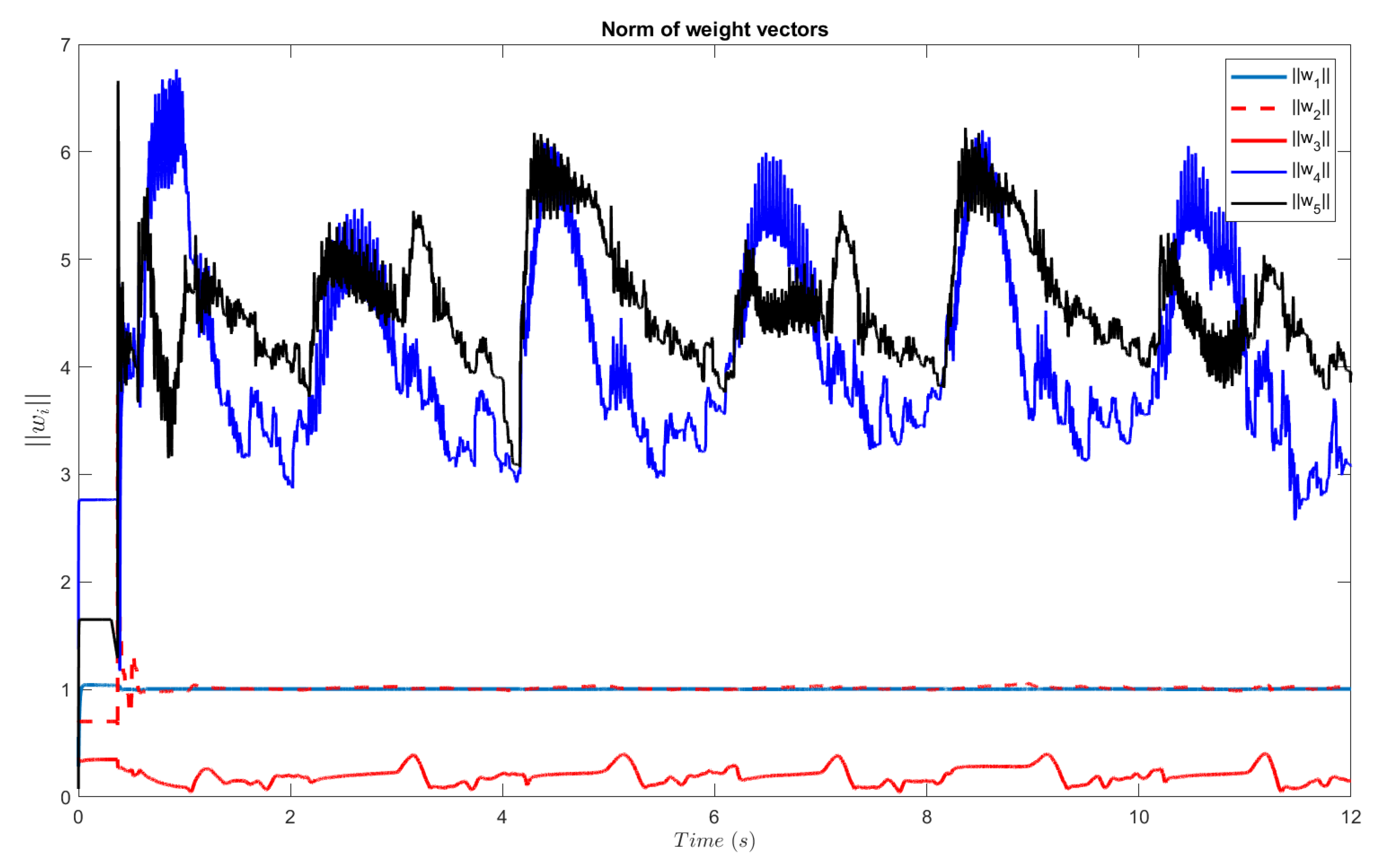
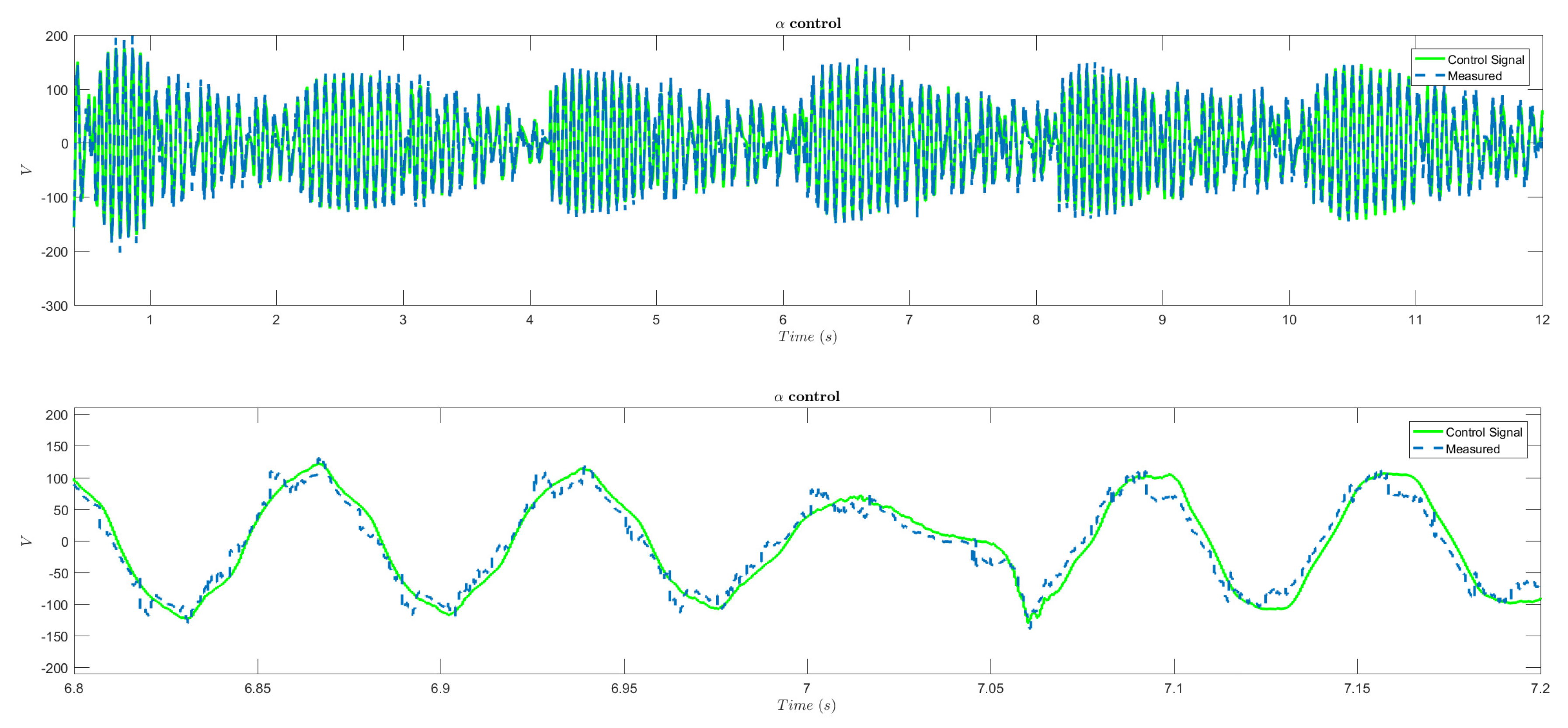
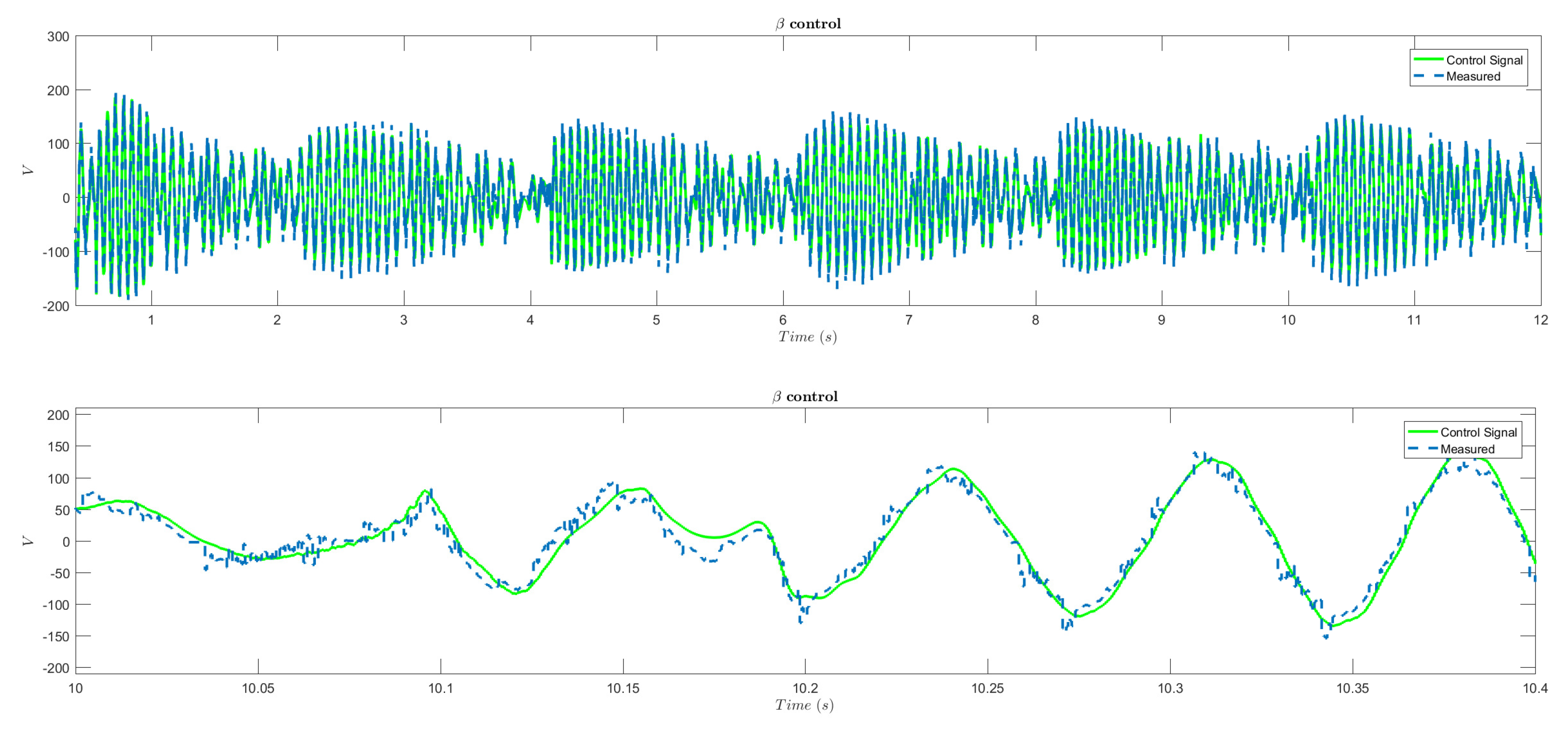
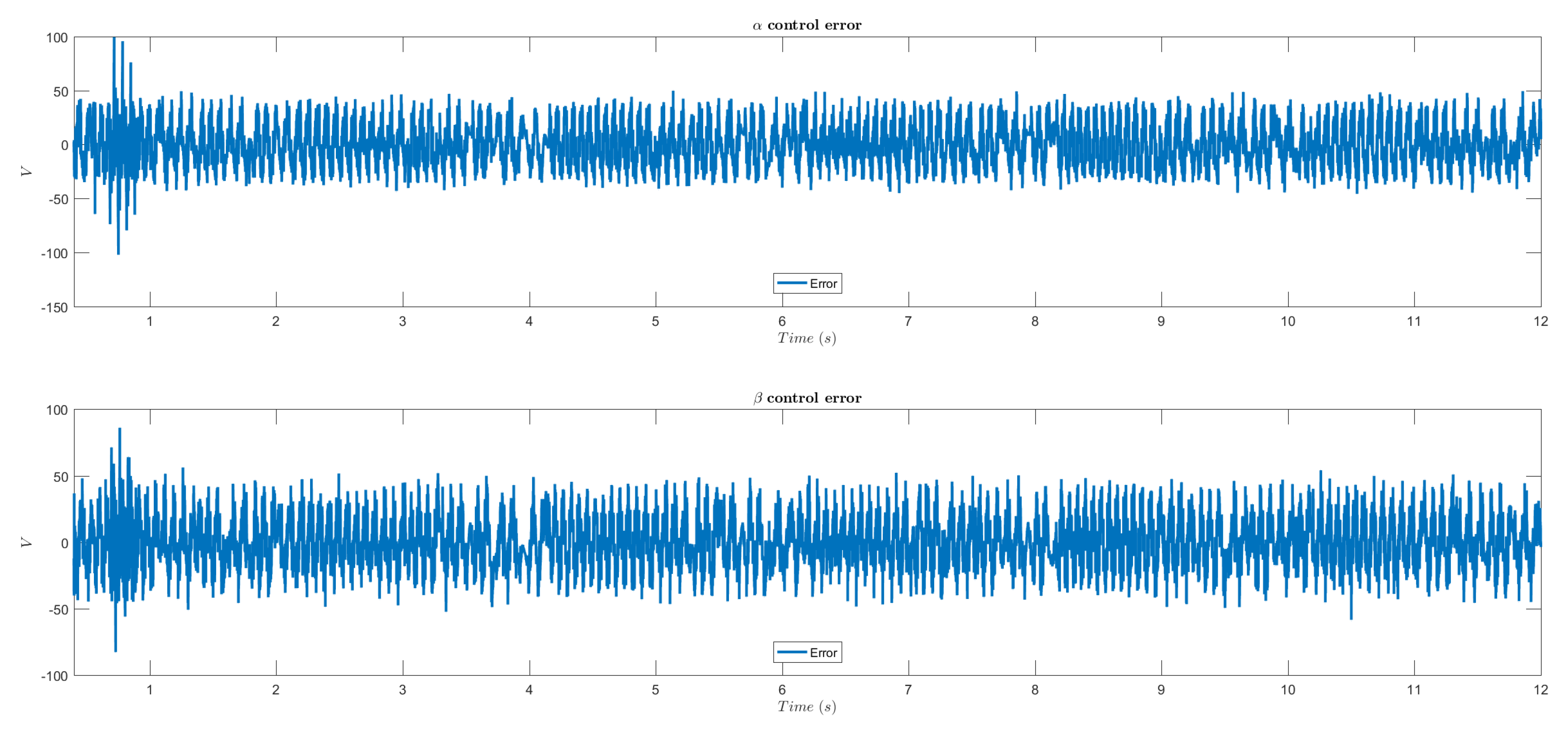
It is easy to see that the identifier in (53) is written as an affine system, as given by (1). Using the obtained model for the identifier, the system can be represented by the following blocks

$$\begin{array}{ccc}\hfill {\widehat{X}}_1\left(k+1\right)& =& {\widehat{x}}_1\left(k+1\right),\hfill \end{array}$$

(55)

$$\begin{array}{ccc}\hfill {\widehat{X}}_2\left(k+1\right)& =& \left[\begin{array}{c}{\widehat{x}}_2\left(k+1\right)\\ {\widehat{x}}_3\left(k+1\right)\end{array}\right],\hfill \end{array}$$

(56)

$$\begin{array}{ccc}\hfill {\widehat{X}}_3\left(k+1\right)& =& \left[\begin{array}{c}{\widehat{x}}_4\left(k+1\right)\\ {\widehat{x}}_5\left(k+1\right)\end{array}\right].\hfill \end{array}$$

(57)

Then, considering the desired trajectory ${\widehat{X}}_{1d}$ for ${\widehat{X}}_1$, the system can be represented as (58)–(60).

$$\begin{array}{ccc}\hfill {\psi }_1\left(k+1\right)& =& {\widehat{X}}_1\left(k+1\right)-X_{1_d}\left(k+1\right)={\widehat{x}}_1\left(k+1\right)-x_{1_d}\left(k+1\right),\hfill \end{array}$$

(58)

$$\begin{array}{ccc}\hfill {\psi }_2\left(k+1\right)& =& {\widehat{X}}_2\left(k+1\right)-X_{2_d}\left(k+1\right)=\left[\begin{array}{c}{\widehat{x}}_2\left(k+1\right)-x_{2_d}\left(k+1\right)\\ {\widehat{x}}_3\left(k+1\right)-x_{3_d}\left(k+1\right)\end{array}\right],\hfill \end{array}$$

(59)

$$\begin{array}{ccc}\hfill {\psi }_3\left(k+1\right)& =& {\widehat{X}}_3\left(k+1\right)-X_{3_d}\left(k+1\right)=\left[\begin{array}{c}{\widehat{x}}_4\left(k+1\right)-x_{4_d}\left(k+1\right)\\ {\widehat{x}}_5\left(k+1\right)-x_{5_d}\left(k+1\right)\end{array}\right].\hfill \end{array}$$

(60)

For this implementation, $X_{1_d}$ is the desired position trajectory, $X_{2_d}$ is defined as $X_{2_d}=\left[x_{2_d},x_{3_d}\right]$, where $x_{2_d}$ (v reference) is determined as

$$\begin{array}{ccc}\hfill k_1{\psi }_1\left(k\right)& =& f_1\left(\overline{x}\left(k\right)\right)+g_1\left(\overline{x}\left(k\right)\right){\overline{x}}_2\left(k\right)-X_{1_d}\left(k+1\right),\hfill \\ \hfill k_1{\psi }_1\left(k\right)& =& w_{f_1}^{\top }\left(k\right)z_{f_1}\left(\overline{x}\left(k\right)\right)+w_{g_1}{\overline{x}}_2\left(k\right)-X_{1_d}\left(k+1\right),\hfill \\ \hfill X_{2_d}\left(x\left(k\right)\right)& =& w_{g_1}^{-1}\left[-w_{f_1}^{\top }\left(k\right)z_{f_1}\left(\overline{x}\left(k\right)\right)+k_1{\psi }_1\left(k\right)+X_{1_d}\left(k+1\right)\right],\hfill \end{array}$$

and $x_{3_d}$ ($\mathsf{\Psi }$ reference) is the given flux magnitude reference; the $X_{3_d}$ reference is defined as $X_{3_d}=\left[x_{4_d},x_{5_d}\right]$, which gives both the $\alpha$ and $\beta$ current references and is computed as

$$\begin{array}{ccc}\hfill k_2{\psi }_2\left(k\right)& =& f_2\left(\overline{x}\left(k\right)\right)+g_2\left(\overline{x}\left(k\right)\right)X_3\left(k\right)-X_{2_d}\left(k+1\right),\hfill \\ \hfill k_2{\psi }_2\left(k\right)& =& w_{f_2}^{\top }\left(k\right)z_{f_2}\left(\overline{x}\left(k\right)\right)+w_{g_2}{X}_3\left(k\right)-X_{2_d}\left(k+1\right),\hfill \\ \hfill X_{3_d}\left(x\left(k\right)\right)& =& w_{g_2}^{-1}\left[-w_{f_2}^{\top }\left(k\right)z_{f_2}\left(\overline{x}\left(k\right)\right)+k_2{\mathsf{z}}_2\left(k\right)+X_{2_d}\left(k+1\right)\right].\hfill \end{array}$$

Finally, the schematic representation for the calculation of u used in (5) is presented in Figure 5.

Remark 4.

The LIM prototype used to test in real time the proposed controller can be modeled by a RHONN, which can be designed in an affine block controllable form composed of two blocks. The first block contains the two desired signals to be controlled, which are controlled by virtual controllers (controllers that are not physically applied to the LIM). These virtual controllers are designed as a feedback linearization system in a block control form whose last block is controlled using an inverse optimal controller to achieve trajectory tracking, minimizing a functional cost criteria [23].

4.3. Results

The following results were obtained from a real-time testing prototype using a LIM; the complete setup is shown in Figure 4. The proposed scheme is programmed in Matlab\Simulink^®(Matlab and Simulink are registered trademarks of MathWorks), and then loaded to a dSPACE^®(dSPACE is a registered trademark of dSPACE GmbH) 1104R&D board, mounted on the PC equipment (Figure 4a), which computes the proposed controller–identifier algorithm using all the information coming from the prototype; all its inputs and outputs go through the connector panel. The dSPACE^® ControlDesk^®(ControlDesk is a registered trademark of dSPACE GmbH) software is used to visualize and store the input and output signals, as well as managing the LIM prototype.

The test is performed in real time on a LIM prototype, using the dSPACE^® 1104R&D controller board with a sampling time equal to 0.3 ms. Blocks to induce delays in the signals during the test are programmed, and they are activated at 4 s, 7 s and 11 s for the position, $\alpha$ current, and $\beta$ current signals, respectively. These blocks randomly substitute the information of the most recent sample with the information form one of the previous ten samples; moreover, each delaying block performs this operation independently from one another in a way that the number of samples that each signal is delayed is chosen randomly as well.

The control objective of the test is the tracking of a trapezoidal reference and the performance is shown in Figure 6, where two zoomed graphs are also presented with intervals 6.8 s to 7.2 s and 10 s to 10.4 s. Figure 7, shows trajectory tracking error for position. Figure 8, shows norm of weight vectors of identifier (53) confirming their boundedness as stated in Theorem 3. From Figure 6 and Figure 7 it can be observed that the measured signal closely follows the reference, clearly establishing the excellent behavior of the proposed controller, moreover, it can also be seen that the measured and identified waveforms are superimposed to one another, which also verifies the superior performance of the proposed identifier structure.

From results depicted in Figure 6 and Figure 7, it is easy to see that the obtained trajectory tracking results are SGUUB, due to the boundedness of the trajectory tracking error depends of the unknown bounds of all the error sources, like quantization error, unmodeled dynamics, uncertainties, disturbances, sensor noises, among others. All these unknown quantities contribute to trajectory tracking error, consistent with the result obtained in Theorem 3 regarding SGUUB [23].

In this paper, a stressing profile for the position has been used to show the applicability and relevance of the proposed controller, showing significant results for real-time trajectory tracking of nonlinear systems, which is not easily found in previous works of quantized systems.

The time instances shown in Figure 6 coincide with the ones of the zoomed graphs in Figure 9 and Figure 10, where both the $u_{\alpha }$ and $u_{\beta }$ components computed by the proposed controller are compared against the $\alpha$ and $\beta$ components of the LIM input voltage, measured in volts (V), at its terminals by voltage sensors. The zoomed images are presented to give an insight into the quantization effects, measurement noise, and delays. It is important to note that the measured signals are converted to $\alpha -\beta$ quantities in the controller board, and then compared with the ones calculated by the proposed controller.

Figure 11 shows two graphs corresponding to the differences between the computed control signals and the ones obtained from measurements of the prototype. It must be noticed that this difference remains bounded and that even though the difference is relatively significant, the performance of our proposed discrete-time neural control scheme is as expected. This can be verified from Figure 7, where the tracking error of the reference trapezoidal signal from Figure 6 is shown to be very small. It is worth noting that the effects considered (quantization from the analog to digital conversion of the measured signals, noise introduced by the measurement sensors, and the induced delay, which can represent a delay of up to ten samples) do not represent conditions that diminish the excellent performance of the proposed controller.

It is important to consider that the proposed identifier has an excellent performance, such that in Figure 6 is almost impossible to note differences between plant state variables and RHONN ones; therefore, to measure such differences, their statistical information is included in

Table 2. Identification root mean square errors.

State Variable	RMSE
$x_1$	$0.000153$ m
$x_2$	0000607 m/s
$x_3$	$0.004495$ Wb2
$x_4$	$1.88391$ A
$x_5$	$1.3332866$ A

. As can be seen from Table 2, the identification errors are small enough to confirm the validity and accuracy of the RHONN-based identifier model for the LIM, in actual operating conditions and with real-life effects considered. In order to further support this claim, the identification RMSE of the state variables from the LIM system are given in Table 2. These errors correspond to the difference between ${\overline{x}}_i-{\widehat{x}}_i$; meanwhile, the flux errors are described by the difference between the observed flux signal and the identified flux signal; all RMSE values are calculated for the 12 s window of the test. As can be seen from Table 2, the identification errors are small enough to confirm the validity and accuracy of the RHONN-based identifier model for the LIM, in actual operating conditions and with real-life effects considered.

4.4. Comparative Analysis

To compare the proposed controller against existing ones,

Table 3. Position tracking error information.

Controller	Mean Value (m/s)	Standard Deviation (m/s)
OTC [29]	0.027393	0.04821
SMC [30]	0.008358	0.09212
NIOCNO [22]	0.002468	0.04703
NIOC	0.001023	0.00763

, displays the mean value and standard deviation for speed tracking error, to a comparison between an optimal tracking control (OTC) [29], a conventional discrete-time sliding mode control (SMC) scheme [30], a NIOC with a neural observer (NIOCNO) [22] with respect to the proposed Quantized NIOC. It is shown that the proposed Quantized NIOC presents the best performance.

4.5. Discussion about Experimental Environment

Real-time implementations involve major challenges caused by unknown dynamics, actuator limitations, quantization errors, unknown delays, and disturbances that can be magnified by the prototype components shown in Figure 11; all these components affect the algorithm. However, all these effects are absorbed and compensated by the proposed identifier-controller approach, as has been displayed by results of Section 4.3 and comparative analysis of Section 4.4. To exemplify this kind of effects, most of them are explained for each of the prototype components:

• Voltage and current sensors are characterized by the presence of noise, measurement error, and quantization error.
• IGBT module has a limited frequency of operation as well as the AC power supply saturates its output. Moreover, the IGBT module has its controllers for IGBTs, which provoke unknown dynamics.
• TTL to CMOS converter, cause noise, uncertainties and unknown dynamics and quantization effects.
• Computer equipment and dSPACE^® 1104 board, presents quantization effects mainly due to the signal conversions at input and output and unknown dynamics provoked by inner circuits.
• LIM contains high nonlinear behaviors, including end effects and unknown uncertainties, mainly due to winding heating, unknown dynamics, hysteresis effects, and parasitic currents, among unknown disturbances by mass effects and the presence of friction, among others. Moreover, this kind of system does not exhibit evident delays effects. However, in this experiment, the delays have been externally included through a time-delay MATLAB^® block, as explained in Section 4.3.

These effects can be easily seen in Figure 10, which shows control error signals between desired control signals and measured signals. Therefore, this paper presents real-time implementation of the controller when simultaneously considering, disturbances, noise, delays, actuator limitations, and quantization for a system with unknown plant model

These are common problems for real-life implementations, and their consequences can be observed in the results included above in this section. Figure 6 and Figure 7 show that due to the capabilities of the RHONN as an identifier (53), it can replicate LIM dynamics, with small identification errors, as shown in Table 2. In Figure 9 and Figure 10 depict the $\alpha -\beta$ components of the calculated control law and the components of the actual measured signal. The difference is presented in Figure 11. This notable error is the consequence of all the phenomena mentioned above, among others. However, meaningful capabilities of the proposed NIOC scheme allow us to obtain good performance for trajectory tracking as is shown in the results depicted in Figure 6 and Figure 7, accompanied of the statistical information included in Table 3 for identification RMSEs, even without the need for previous knowledge of a model for the controlled system nor an explicit estimation of its bounds. In order to explain the nature of the above-mentioned effects, in Figure 12 schematic representation of the control signal route is included, from the calculated value of vector $u\left(k\right)$ along with its application to the LIM prototype and its measurement for $\alpha -\beta$ components calculation to be depicted in Figure 9, Figure 10 and Figure 11.

5. Conclusions

This work reports a complete neural identifier-control model that deals with quantization error, measurement noise, disturbances, uncertainties, and signal delays. For any such conditions, it is not necessary to know neither the nominal model nor its estimations or bounds. The proposed controller is applied to an actual LIM in a real-time experimental test, which shows that the identification errors for all the state variables and the trajectory tracking errors are small enough. The presented results were obtained working with a LIM without knowledge of its model or parameters.

It is important to note that the experimental test intrinsically considers quantization error, measurement noise, disturbances, uncertainties, and delay. However, an additional delay of up to ten samples is randomly applied to the position, $\alpha$ current, and $\beta$ current signals. Despite all this, the proposed neural identifier-control scheme shows an excellent real-time performance with a sample time equal to 0.3 ms. As seen from the results, the tracking of the reference signal is effectively achieved even though a trapezoidal waveform represents a difficult task for a LIM.

Moreover, a Lyapunov analysis is included with the proof of the semi-globally uniformly ultimately boundedness (SGUUB) of the proposed scheme. Furthermore, it must be noticed that the stability proof requires neither persistent excitation condition nor separation principle relaxing conditions to achieve boundedness of the entire identifier-control scheme. Proposed results can be extended for systems with hysteresis, backlash, friction, and other interesting problems.

For the experimental results included in this paper, controller parameters have been heuristically selected. However, as future work, authors consider the use of an evolutionary algorithm to define an auto-tuning approach.

References

1. Alanis, A.Y.; Rios, J.D.; Arana-Daniel, N.; Lopez-Franco, C. Neural identifier for unknown discrete-time nonlinear delayed systems. Neural Comput. Appl. 2016, 27, 2453–2464. [Google Scholar] [CrossRef]
2. Rios, J.D.; Alanis, A.Y.; Lopez-Franco, C.; Arana-Daniel, N. RHONN identifier-control scheme for nonlinear discrete-time systems with unknown time-delays. J. Frankl. Inst. 2018, 355, 218–249. [Google Scholar] [CrossRef]
3. Zhang, D.; Han, Q.; Zhang, X. Network-Based Modeling and Proportional–Integral Control for Direct-Drive-Wheel Systems in Wireless Network Environments. IEEE Trans. Cybern. 2020, 50, 2462–2474. [Google Scholar] [CrossRef] [PubMed]
4. Zhang, D.; Zhou, Z.; Jia, X. Networked fuzzy output feedback control for discrete-time Takagi–Sugeno fuzzy systems with sensor saturation and measurement noise. Inf. Sci. 2018, 457–458, 182–194. [Google Scholar] [CrossRef]
5. Okuyama, Y. Discrete Control Systems; Springer: London, UK, 2014. [Google Scholar]
6. Kalman, R.E. Nonlinear aspects of sampled-data control systems. In Proceedings of the Symposium on Nonlinear Circuit Analysis VI; Polytechnic Institute of Brooklyn: Brooklyn, NY, USA, 1956; pp. 273–313. [Google Scholar]
7. Xia, Y.; Fu, M.; Liu, G. Analysis and Synthesis of Networked Control Systems; Lecture Notes in Control and Information Sciences; Springer: Berlin/Heidelberg, Germany, 2011. [Google Scholar]
8. Isidori, A. Nonlinear Control Systems; Communications and Control Engineering; Springer: London, UK, 2013. [Google Scholar]
9. Khalil, H. Nonlinear Systems; Pearson Education, Prentice Hall: Upper Saddle River, NJ, USA, 2002. [Google Scholar]
10. Liu, Y.; Peng, Y.; Wang, B.; Yao, S.; Liu, Z. Review on cyber-physical systems. IEEE/CAA J. Autom. Sin. 2017, 4, 27–40. [Google Scholar] [CrossRef]
11. Chen, G. Pinning control and controllability of complex dynamical networks. Int. J. Autom. Comput. 2017, 14, 1–9. [Google Scholar] [CrossRef]
12. Salgado, I.; Ahmed, H.; Camacho, O.; Chairez, I. Adaptive sliding-mode observer for second order discrete-time MIMO nonlinear systems based on recurrent neural-networks. Int. J. Mach. Learn. Cybern. 2019, 10, 2851–2866. [Google Scholar] [CrossRef]
13. Li, L.; Zheng, N.; Wang, F. On the Crossroad of Artificial Intelligence: A Revisit to Alan Turing and Norbert Wiener. IEEE Trans. Cybern. 2019, 49, 3618–3626. [Google Scholar] [CrossRef]
14. Wu, W.; Wang, C.; Yuan, C. Deterministic learning from sampling data. Neurocomputing 2019, 358, 456–466. [Google Scholar] [CrossRef]
15. Liu, C.; Liu, X.; Wang, H.; Zhou, Y.; Lu, S. Observer-based adaptive fuzzy funnel control for strict-feedback nonlinear systems with unknown control coefficients. Neurocomputing 2019, 358, 467–478. [Google Scholar] [CrossRef]
16. Xi, C.; Dong, J. Adaptive neural network-based control of uncertain nonlinear systems with time-varying full-state constraints and input constraint. Neurocomputing 2019, 357, 108–115. [Google Scholar] [CrossRef]
17. Chang, X.; Xiong, J.; Li, Z.; Park, J.H. Quantized Static Output Feedback Control For Discrete-Time Systems. IEEE Trans. Ind. Inform. 2018, 14, 3426–3435. [Google Scholar] [CrossRef]
18. Xu, H.; Zhao, Q.; Jagannathan, S. Finite-Horizon Near-Optimal Output Feedback Neural Network Control of Quantized Nonlinear Discrete-Time Systems With Input Constraint. IEEE Trans. Neural Netw. Learn. Syst. 2015, 26, 1776–1788. [Google Scholar] [CrossRef] [PubMed]
19. Wang, Y.; Shen, H.; Duan, D. On Stabilization of Quantized Sampled-Data Neural-Network-Based Control Systems. IEEE Trans. Cybern. 2017, 47, 3124–3135. [Google Scholar] [CrossRef] [PubMed]
20. Zhou, J.; Wang, W. Adaptive Control of Quantized Uncertain Nonlinear Systems. IFAC-PapersOnLine 2017, 50, 10425–10430. [Google Scholar] [CrossRef]
21. Wang, C.C.; Yang, G.H. Prescribed performance adaptive fault-tolerant tracking control for nonlinear time-delay systems with input quantization and unknown control directions. Neurocomputing 2018, 311, 333–343. [Google Scholar] [CrossRef]
22. Lopez, V.G.; Sanchez, E.N.; Alanis, A.Y.; Rios, J.D. Real-time neural inverse optimal control for a linear induction motor. Int. J. Control. 2017, 90, 800–812. [Google Scholar] [CrossRef]
23. Sanchez, E.; Ornelas-Tellez, F. Discrete-Time Inverse Optimal Control for Nonlinear Systems; CRC Press: Boca Raton, FL, USA, 2017. [Google Scholar]
24. Rovithakis, G.; Christodoulou, M. Adaptive Control with Recurrent High-Order Neural Networks: Theory and Industrial Applications; Advances in Industrial Control; Springer: London, UK, 2012. [Google Scholar]
25. Boldea, I.; Nasar, S. Linear Electric Actuators and Generators; Cambridge University Press: Cambridge, UK, 2005. [Google Scholar]
26. Takahashi, I.; Ide, Y. Decoupling control of thrust and attractive force of a LIM using a space vector control inverter. IEEE Trans. Ind. Appl. 1993, 29, 161–167. [Google Scholar] [CrossRef]
27. Levin, A.U.; Narendra, K.S. Control of nonlinear dynamical systems using neural networks: Controllability and stabilization. IEEE Trans. Neural Netw. 1993, 4, 192–206. [Google Scholar] [CrossRef]
28. Sanchez, E.; Alanís, A.; Loukianov, A. Discrete-Time High Order Neural Control: Trained with Kalman Filtering; Studies in Computational Intelligence; Springer: Berlin/Heidelberg, Germay, 2008. [Google Scholar]
29. Ornelas-Tellez, F.; Alanis, A.Y.; Rios, J.D.; Graff, M. Reduced-order observer for state-dependent coefficient factorized nonlinear systems. Asian J. Control. 2019, 21, 1216–1227. [Google Scholar] [CrossRef]
30. Alanis, A.Y.; Rios, J.D.; Rivera, J.; Arana-Daniel, N.; Lopez-Franco, C. Real-time discrete neural control applied to a Linear Induction Motor. Neurocomputing 2015, 164, 240–251. [Google Scholar] [CrossRef]
Figure 1. Schematic representation for neural identification of discrete-time unknown nonlinear quantized delayed systems with measurement noise.
Electronics 09 01274 g001
Figure 2. Schematic closed-loop system representation of a discrete-time unknown nonlinear quantized delayed system with measurement noise.
Electronics 09 01274 g002
Figure 3. Scheme of a NIOC.
Electronics 09 01274 g003
Figure 4. Linear induction motor (LIM) prototype. (a) Computer with dSPACE® software and RTI 1104 board installed, (b) dSPACE® RTI 1104 panel connector, (c) Linear induction motor, (d) Voltage sensor, (e) Current sensor, (f) Power supply, (g) TTL to CMOS converter, (h) encoder, (i) IGBT module (or insulated-gate bipolar transistor), (j) Auto-transformer.
Electronics 09 01274 g004
Figure 5. Schematic representation for control law calculation.
Electronics 09 01274 g005
Figure 6. Tracking performance of our proposed neural control scheme for a trapezoid signal and zoomed images at the same time intervals of the zoomed images of the control signals.
Electronics 09 01274 g006
Figure 7. Position tracking error.
Electronics 09 01274 g007
Figure 8. Norm of weight vectors.
Electronics 09 01274 g008
Figure 9. Control signal u α from the test and the zoomed image for a time interval from 6.8 s to 7.2 s.
Electronics 09 01274 g009
Figure 10. Control signal u β from the test and the zoomed image for a time interval from 10 s to 10.4 s.
Electronics 09 01274 g010
Figure 11. Control error signals between desired control signals and measured signals.
Electronics 09 01274 g011
Figure 12. Control signal route: From calculated to applied signal.
Electronics 09 01274 g012